1. Introduction
Control algorithms for a wind turbine are generally designed to control both power and load [
1]. The power control includes the maximum power region at wind speed lower than the rated wind speed, the rated power region at wind speed higher than the rated wind speed, and the transition region between the two mentioned power control regions. These control regions are named region 2, 3, and 2.5, respectively [
2]. The load control is targeted to reduce loads that the wind turbine experiences and is distinguished on the basis of the load that is mostly reduced [
3,
4]. The tower damper is known to reduce the tower load and uses the acceleration signal of the nacelle to calculate the command to the pitch actuator to reduce loads [
4,
5,
6,
7,
8,
9]. This is used in region 3. The peak shaving is known to reduce the tower and blade loads at region 2.5 by slightly adjusting the pitch angle of the blade by a pre-designed pitch schedule [
10]. The individual pitch control is used in region 3 to reduce the blade load due to imbalance loads caused by wind shear, tower shadow, etc. It uses the signals from strain sensors mounted on the blade roots to calculate the command to the pitch actuator [
4,
11]. The drivetrain damper is used in region 2 to reduce the low-speed shaft torque due to torsional modes from the drive train [
12]. It uses the generator speed signal to calculate the torque command to the generator to cancel out the drivetrain mode in the torque command.
Power control for modern wind turbines is achieved by a combination of open-loop and closed-loop control. In region 2, the control strategy is to maximize the wind turbine power, and this is achieved by an open-loop torque control with a fixed pitch angle (known as fine pitch) to maximize the power coefficient which is the aerodynamic conversion efficiency of the rotor. Either a generator torque–speed lookup table or an optimal mode gain (optimal relationship between generator speed and torque) is used for this [
13,
14]. The power control in region 2.5 is an extension of the power control in region 2, and the control strategy just performs a smooth transition from region 2 to region 3. The control strategy in region 3 consists in regulating the power so that it does not exceed the rated power of the wind turbine. The generator speed is controlled by either a PI (proportional-integral) or a PID (proportional-integral-differential) control to achieve the rated wind speed. The generator torque is controlled by open-loop control and PI control [
4,
15].
Although many modern control algorithms, including the linear quadratic regulator (LQR), fuzzy control, and model predictive control (MPC) algorithms, have been proposed by researchers as control algorithms for wind turbines to improve their performance [
16,
17,
18,
19,
20], no algorithm has been chosen as an alternative to the conventional PI or PID power control by wind turbine manufacturers or companies to provide wind turbine control solutions. This is because the conventional PI or PID control algorithms for wind turbines have been used for a long time as power control algorithms and found to be robust and effective. This practice is not likely to change fast, as manufacturers often adopt a conservative approach towards innovation in control system design.
Efforts have been made to improve the performance of the conventional PI or PID control algorithms by adding extra commands to the calculated pitch command [
21,
22]. These methods measure the wind speed by Light Detection and Ranging (LIDAR) or by other techniques; they commonly use the partial derivative of the pitch angle with respect to the generator speed to calculate the required pitch angle variation based on the current wind speed variation and add this, multiplied by a suitable proportional gain, to the pitch command from the conventional PI or PID control algorithm. Although these feed-forward controls could not be validated, they are considered to be applicable to the actual wind turbines because they use the conventional PI or PID control algorithms as a basis and integrate the feed-forward control in region 3.
This study was performed to develop a new power control algorithm to be applied to a 100 kW medium-capacity wind turbine to improve its performance using a similar approach to the previous feed-forward control. The target wind turbine is not a multi-megawatt wind turbine and cannot afford a LIDAR to measure the wind speed, therefore a wind speed estimator was chosen for this study. Also, to calculate the feed-forward pitch command signal, contributions from other measured parameters as well as the estimated wind speed were considered for fine adjustment of the pitch angle command that was added to the command from the conventional PI or PID control algorithm. Therefore, an LQR controller was finally selected for this purpose. The LQR control uses wind speed estimators to estimate the representative wind speed experienced by that wind turbines and determine the magnitude of the control command [
21,
23,
24,
25,
26]. Reference [
24] constructed a tower and blade state estimator using accelerometers and strain gauges arranged along structural members and used it to estimate the wind state. The demonstration was conducted through an aerosol-servo-elastic simulator, which suggested that the individual blade fatigue and load could be reduced. Reference [
25] demonstrated power curve tracking through a model-based control using a wind schedule for 3 MW wind turbines with blade tip speed constraints in simulated environments. In Reference [
26], a wind observer was tested using field test data collected from NREL CART3 wind turbines. The results showed that the rotor equivalent wind speed estimated by the proposed observer correlated with the meteorological data and was much more accurate than the speed measured by an onboard wind vane. The wind speed estimator used in this study used a three-dimensional (3D) lookup table based on the two-mass drivetrain model with measured generator speed, torque, and pitch angle [
4,
21]. In [
16], an LQR controller was designed for a megawatt (MW)-class wind turbine, and simulations were performed to test its performance. The simulation results showed that the performance of the wind turbine was improved by the proposed LQR controller compared to that obtained with the conventional PI control, and the blade and tower loads were also reduced. Reports in the literature show that LQR controllers are effective as wind turbine controllers [
16], but their performance relies on the accuracy of the wind speed estimators, so they are vulnerable to the noise or unexpected events influencing the measurement signal that is used for wind speed estimation. The reason is that the sensitivity varies with the wind speed. This issue has not been studied.
The purpose of this paper was to improve the performance of a PI control algorithm by virtue of an LQR controller which has a good control performance but is vulnerable to uncertainties in wind speed estimation. Therefore, a hybrid controller is newly proposed in this study. A PI control was used as the conventional power control, and an LQR control was used as a feed-forward controller to improve the control performance. This new control algorithm minimizes changes in the conventional PI control algorithm so that it could be relatively easily adopted by wind turbine manufacturers as a new control algorithm for modern wind turbines. Also, the proposed algorithm was expected to limit the contribution from the LQR controller which was significantly affected by wind speed estimation errors because the LQR controller was used as a feed-forward controller. For this, a new hybrid controller, which is a combination of the conventional PI and LQR controllers, was designed for a 100 kW wind turbine. It is difficult to validate wind turbine control algorithms in a field test with multi-MW-class wind turbines. Therefore, numerical modeling is generally used to validate the performance of a single wind turbine or in wind farms [
27,
28,
29,
30,
31,
32]. The target wind turbine had a permanent-magnet synchronous generator (PMSG) without a gearbox and blades with a substantially smaller rotor moment of inertia and faster rotational speed compared to those of MW-class wind turbines. The proposed LQR-PI controller was tested with dynamic simulations, and the performances were compared with those of a PI and an LQR control algorithms with and without noise in the measured generator speed signal.
3. Numerical Modeling
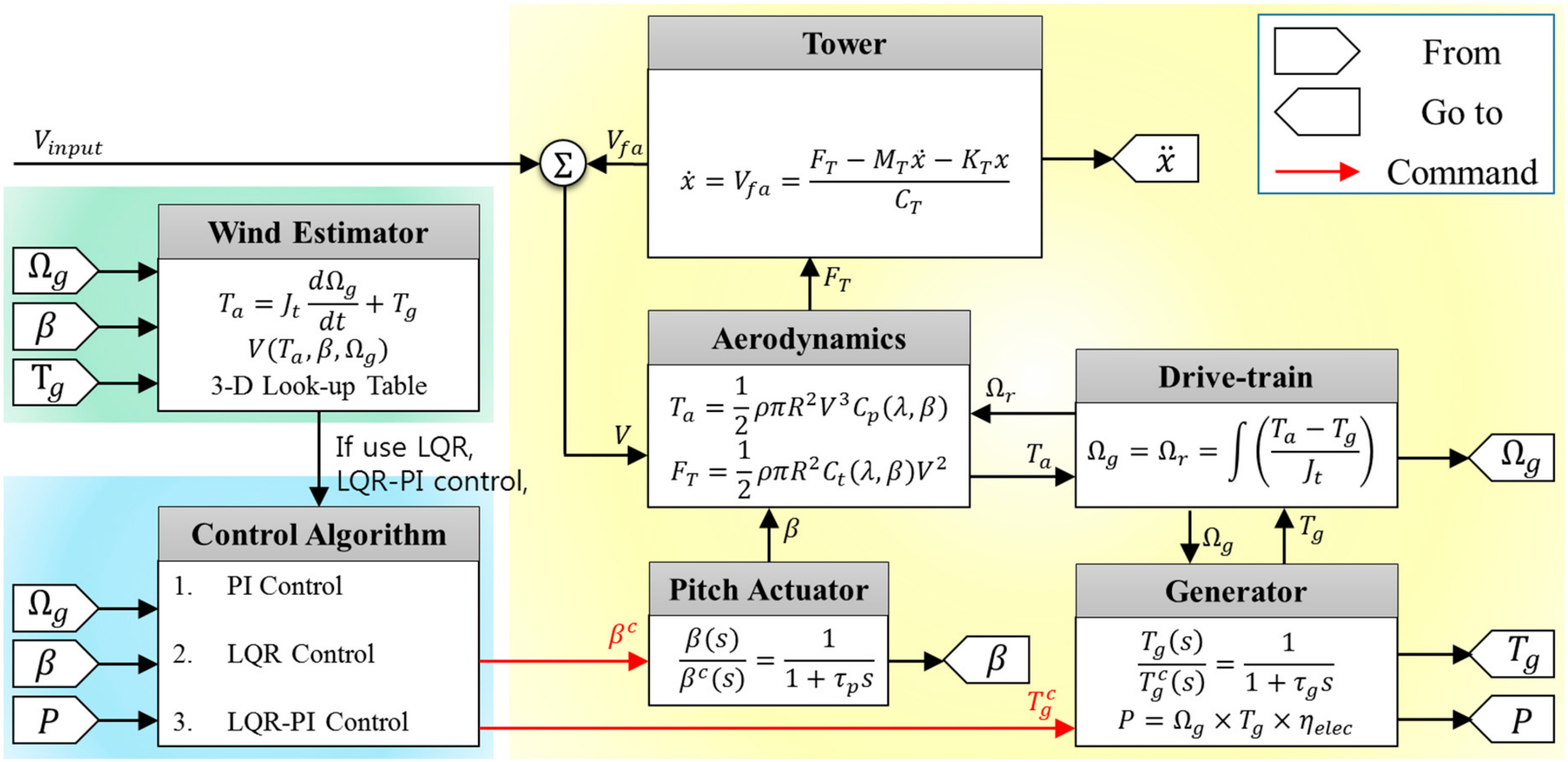
The commercial code DNVGL-Bladed (4.6, DNV·GL, Oslo, Norway) was used for numerical modeling. DNVGL-Bladed was used to extract linear models, blade power coefficients, and thrust coefficients for the wind turbine. The in-house code includes control algorithms, wind speed estimators, and wind turbine numerical models. This section describes the wind speed estimator and wind turbine numerical models, and the next section introduces the control algorithm. From a control system perspective, a wind turbine numerical model includes aerodynamics, drive trains, generators, towers, and pitch actuators.
A block diagram of the overall functional scheme of a wind turbine is shown in
Figure 2. The blue box indicates the control algorithm, the green box indicates the wind speed estimator, and the yellow box presents the wind turbine numerical model.
3.1. Aerodynamics
The aerodynamics model makes use of power coefficient and thrust coefficient lookup tables extracted as a function of the pitch angle and tip speed ratio (TSR) through the aerodynamic analysis of DNVGL-Bladed. In this component, the wind speed, generator speed, and pitch angle are the input. The aerodynamic torque and thrust force are calculated through Equations (1) and (2), respectively, and applied to the drivetrain and tower model, respectively.
3.2. Drivetrain
The target wind turbine is a PMSG type without a gearbox, so Equation (3) can be derived from
Figure 3. This component receives the generator torque and aerodynamic torque from a generator and aerodynamics model, calculates the generator speed, and delivers it back to the aerodynamics and generator model.
3.3. Generator
The generator can be simplified to Equation (4) from the side of the control system. The torque command and generator speed are input from the control algorithm and the drivetrain model, respectively, to calculate the generator torque and electrical power. The electrical power is calculated using Equation (5).
3.4. Tower
The tower model is expressed as the equation of motion given in Equation (6). In this model, the velocity at which the nacelle sways fore and aft because of the wind speed is added to the input wind speed and entered into the aerodynamics model.
3.5. Pitch Actuator
The dynamic characteristics of the pitch actuator model are expressed by Equation (7). The pitch actuator operates within the limits of Equations (8) and (9) according to the design specification.
4. Control Algorithms
This section introduces PI control, LQR control, and LQR-PI hybrid control algorithms. The PI control algorithm is a control technique applied to the target wind turbines and in this study, it is presented as a reference control algorithm to compare the performance of LQR control and LQR-PI control.
4.1. PI Control Algorithm
The PI control algorithm adopted and used by the target wind turbine receives feedback on the measured pitch angle, electrical power, and generator speed, and sends pitch angle and torque commands to the pitch actuator and generator [
7,
10,
15]. In practice, mechanical load-reduction control techniques such as tower dampers and peak shaving are usually applied, but in this study, only power control was considered.
Figure 4 shows a block diagram of the pitch PI control algorithm containing the gain schedule. The configuration consists of a pitch PI control, torque schedule, and mode switch. The torque schedule is a lookup table with an input of generator speed and an output of generator torque. It was constructed to perform an open-loop maximum power point tracking (MPPT) control to achieve the optimal tip speed ratio with the measured generator speed in region 2. The optimal values of the generator torque with respect to the input generator speeds were calculated on the basis of the aerodynamic analysis of the rotor using DNVGL-Bladed. The gain selection of pitch PI control and operation of the mode switch are explained in detail below.
Figure 5 shows the block diagram of the mode switch. The mode switch determines the control mode using an internal logic with the measurement values of generator speed, electrical power, and pitch angle. A set-reset (SR) flip-flop is a logic that remembers one bit and remains in the current state until a change in the state signal (clock) is generated. If the measured generator speed or power exceeds the rated values, the mode switch outputs a signal of 1 (switched on). Also, the mode switch outputs a signal of 1 (switched on) if the measured pitch angle is greater than the fine pitch angle.
When the mode switch is on, pitch PI control is performed, and the generator torque command is fixed to be the rated value. When the mode switch is off, to perform open-loop MPPT control, the pitch angle command is fixed to be the fine pitch angle, and the torque control is performed through the torque schedule.
Figure 6 shows the frequency response of the pitch control loop gain.
Figure 6a shows the frequency response of the open-loop transfer function given in Equation (10). The frequency response was drawn over all the wind speeds from the rated wind speed to the cutout wind speed by 0.5 m/s intervals. As shown in the figure, the frequency response varies depending on wind speed. Therefore, to have uniform pitch sensitivity, gain scheduling should be applied to maintain a constant value of the cross frequency of the pitch control loop. In this study, the cross frequency was set to 1 rad/s, taking into account the fact that most energy components in wind speed exist at frequencies lower than 1 rad/s based on the power spectrum of wind speed [
4].
Figure 6b shows the frequency response of the pitch control loop gain transfer function of Equation (11). The pitch control loop consists of gain scheduling, PI control, pitch actuator dynamics (Equation (7)) and open-loop transfer function (Equation (10)). As shown in the figure, all the frequency responses (magnitude plot) at different wind speeds had a cross frequency of 1 rad/s, and the phase margin (phase plot) of at least 30 degrees was achieved for system stability.
4.2. LQR Control Algorithm
Figure 7 shows the control structure of the LQR control algorithm. The pitch control was replaced by LQR control. The LQR control received the generator speed, torque, and pitch angle as inputs. In addition, the wind speed estimator used the current generator speed, torque, and pitch angle to deliver the estimated wind speed to the designed LQR control. The design of the wind speed estimator is presented in detail in
Section 5.
Linearization models are required to select the optimal gain for LQR control. In this study, a linearization model was acquired through DNVGL-Bladed. In Equation (12), the state matrix A and input matrix B are stabilizable. The state vectors and control vectors are presented in Equation (13). In state vector x, the pitch angle actually reflects only one result because the target wind turbine performs collective pitch control (CPC). In order to stabilize the system Equation (12), the optimum gain K in Equation (17) that minimizes the quadratic cost function (Equation (15)) through the state feedback method (Equation (14)) must be selected. In Equation (17), S is the symmetric positive semidefinite solution of the Riccati Equation (16). Since the size of the matrix was large, K was obtained using the LQR function of MATLAB (R2014a, The MathWorks, Inc, Natick, MA, USA).
Also, the weight matrices
Q and
R that met the conditions in Equation (18) were chosen randomly and simulated by solving the Riccati Equation. Then
Q and/or
R were re-selected if transient response specifications and/or size constraints were not met. This means that the weight matrix was selected as a tuning process until a satisfactory performance was achieved. The
Q matrix was weighted more heavily for the state variables, so that the objective was achieved in a short time, and the
R matrix was chosen through the simulation response.
4.3. LQR-PI Control Algorithm
Figure 8 shows a block diagram of the LQR-PI control algorithm proposed in this paper. The LQR-PI control combines the control output of the PI pitch control and that of the LQR control to transmit the combined pitch command to the pitch actuator. As shown in the figure, the LQR control was applied in this structure as a feedforward term for pitch control.
Although it is simply a combination of LQR control and PI control, both controls can complement each other in the pitch control domain to improve the operating stability of the wind turbine. If the LQR control delivers the optimum pitch angle command to the pitch actuator and performs a sufficiently stable control, the contribution of the PI control will be small, because the pitch PI control will intervene in control when the measured generator speed exceeds the rated value. However, because of noise or unexpected circumstances, the LQR control may send incorrect pitch commands to the pitch actuator, thus not achieving its original purpose of maintaining the rated generator speed. In this case, PI control takes the lead in pitch control.
LQR-PI control was configured to perform a PI control also when LQR control was removed (or disconnected by a switch) from the control structure. The advantage of this feature is that when the LQR-PI control is applied to actual wind turbines, only a feed-forward loop of LQR control can be added to the pitch loop of the existing PI controller without modifying existing control algorithms.
5. Wind Speed Estimator
The nacelle wind speed is not suitable for feeding a control-scheduling logic because it is disturbed by the rotation of the rotor, which introduces a periodic decrease with multiples of the rotor frequency, as well as higher frequency disturbances due to wake turbulence [
33]. Therefore, a wind speed estimator was designed for LQR control and used to calculate the rotor average wind speed.
Figure 9 shows a block diagram of the wind speed estimator. It consists of an aerodynamic torque estimator, a 3D look-up table for wind speed, and a low-pass filter. The aerodynamic torque estimator is just a Simulink representation of Equation (3), which is the two-mass drivetrain model. The aerodynamic torque was firstly estimated from the aerodynamic torque estimator using the rotor speed and the generator torque and then was supplied to the 3D lookup table as an input. Two more inputs of pitch angle and rotor speed were provided to the 3D lookup table to get the wind speed as an output. The wind speed from the 3D lookup table was finally low-pass filtered to remove high-frequency components [
21].
The 3D lookup table in
Figure 9 was created using the fminsearch function of MATLAB. The fminsearch is a function minimization algorithm based on the Nelder-Mead simplex method [
34,
35,
36]. It can be applied to nonlinear functions whose derivatives are not known and is one of the most widely used function minimization algorithms for a direct search method. This method uses a simple value known as a polytope with
n + 1 vertices (or
n + 1 test point) in the
n variable of the objective function. To find a value that can minimize objective function values, compare the function values at the
n + 1 test point, avoid the test points that provide the worst function values, and repeat the reflection, contraction, and extension of the variables [
36].
That is, the fminsearch finds the wind speed to minimize the error between the power calculated and the rated power, as shown in
Figure 10. To calculate the electrical power, the aerodynamic torque was firstly calculated using Equation (1) with inputs of wind speed, rotor speed, and pitch angle. The wind speed, in this case, was a trial value from the fminsearch algorithm, and the others were the given inputs. The aerodynamic torque was finally multiplied by the rotor spee, and the generator loss and converted into electrical power. The error between the calculated power and the rated power was used as a cost function in the fminsearch algorithm to be minimized. At the function minimum, the wind speed could be obtained. The inputs were varied to construct a 3-D lookup table whose output was the wind speed. The inputs in the lookup table were rotor speed, pitch angle, and aerodynamic torque.
Figure 11 shows the results of the 3D lookup table constructed through this process. The 3D lookup table was constructed for the operation range as a function of rotor speed, pitch angle, and estimated aerodynamic torque. For example, if the estimated aerodynamic torque for a given rotor speed of 40 RPM, as in
Figure 11 was 25 kNm and the pitch angle was 14°, the wind speed would be 15 m/s.
To validate the wind speed estimator using simulation, the wind speed estimated from the wind speed estimator was compared with the rotor averaged wind speed from DNVGL-Bladed (
Figure 12). A dynamic simulation at a mean wind speed of 14 m/s was performed with the target wind turbine, and the rotor averaged wind speed was obtained from DNVGL-Bladed. The generator torque, rotor speed, pitch angle from DNVGL-Bladed at a time interval of 10 ms were used as inputs to the wind speed estimator, and the turbulent wind speeds were obtained as outputs. Although a delay of less than 1 second was found, the wind speed estimator considered appeared valid because the mean and the standard deviation of the two wind speed data were almost identical.
6. Simulation
6.1. Method
The simulation was performed for the transition region and the rated power region where pitch control was used. The wind speed calculated through the wind speed estimator was used as the input wind speed for the simulation. For this, the measured generator speed, generator torque, and pitch angle from the target 100 kW wind turbine were used.
Figure 13 shows the wind speed estimated by the measured data, and the nacelle wind speed measured by an anemometer on top of the nacelle.
Figure 13a shows the wind speed of the transition region, and
Figure 13b shows the wind speed of the rated power region. In the case of the nacelle wind speeds, although the speeds actually had a higher frequency, they appeared to be similar to the estimated wind speed because the data measuring device collected data with a sample rate of 1 Hz. Although the nacelle wind speed was affected by the rotor rotation, the estimated wind speed was found to be similar to the nacelle wind speed, and as expected, it was found to be slightly higher than the nacelle wind speed. The mean value and the standard deviation of the input wind speed were 10.58 m/s and 0.98 m/s, respectively, for the transition region, and they were 15.21 m/s and 1.73 m/s, respectively, for the rated power region.
The simulation was performed with three different control algorithms including the conventional PI, the LQR, and the proposed LQR-PI. The simulation was also performed with and without noise to evaluate the controller performance in the presence of noise in the measured signal. In the simulation with noise, randomly mixing Gaussian noise was added to the generator speed.
6.2. Results without Noise
Figure 14a,b show the simulation results without considering noise in two different wind speed regions, i.e., the transition region and the rated power region. They compare the results with the conventional PI, the LQR, and the proposed LQR-PI controller. The simulation was performed for 600 s, but for visibility purposes, only the results from 0 to 100 s are presented. In
Figure 14, the black line for wind speed represents the input wind speed obtained from the previous section. The subplot of wind speed also includes the wind speeds obtained from the wind speed estimators in the simulations with three different controllers. The estimated wind speed obtained by three different controllers showed a difference of less than 1% in mean wind speed compared with input wind speed, but the standard deviations were 4.08% and 3.47% higher for transition and rated power regions, respectively.
In the transition region, the PI control showed the largest overshoot of generator speed. This can be explained in relation to the pitch angle. The PI control regulates the pitch angle from the moment it exceeds the rated generator speed, but the LQR and the LQR-PI controls started the pitch angle in advance to attenuate the generator speed increase. Although the LQR and the LQR-PI controls used the estimated wind speed delayed by about 1 second for their control command calculation, the standard deviation of the generator speed was reduced compared with that obtained with the PI control. Sudden dips in the generator torque and power were observed in the simulation with all three controllers, but the greatest one was obtained with the PI controller. The results with the LQR controller were the best, and that those the LQR-PI were intermediate. On the basis of these results, it was concluded that the overshoot of the power was mostly due to the generator speed, and the dip was mostly due to the generator torque.
For the rated power region, the results with three different controllers were similar, but the lowest standard deviation of the generator speed was achieved when the LQR-PI control was used. Quantitative comparisons of the simulation results are shown in
Table 2 and
Table 3.
Table 2 and
Table 3 show the simulation results for 600 seconds. The most notable performance indicators in the results presented are the standard deviations of the generator speed, which can represent the operating stability of the wind turbine. The estimated wind speed in
Table 2 and
Table 3 represents the estimated wind speed from the wind speed estimator. These were about the same with three different controllers, although the operating points were slightly different.
The results given in
Table 2 indicate that the LQR control reduced the standard deviation of the generator speed by 26.58% compared to the PI control. In the case of the LQR-PI control, the standard deviation of the generator speed was even 16.7% lower than that for the LQR control, and 38.85% less than that for the PI control. However, as a side effect, the mean power with the LQR-PI control was reduced by 0.57% with respect to that measured with the LQR control.
As can be seen in
Table 3, the LQR control and LQR-PI control had less than a 1% difference in all average performance indices compared with the PI control. For the standard deviation, the LQR control had a lower generator speed of 1.15% and a higher pitch angle of 17.63% compared to the PI control. A higher standard deviation of the pitch angle means that the pitch control was busier. The generator torque and power generation increased by 7.41% and 4.9%, respectively. The LQR-PI control reduced the standard deviation of the generator speed by 26.86% compared with the PI control, and the standard deviations of the pitch angle, generator torque, and power increased by 23.13%, 11.63%, and 1.53%, respectively.
As a result, the LQR control was able to increase the stability of wind turbines by reducing the standard deviation of the generator speed. However, in regions where the pitch control was continually used, the effect was reduced. On the other hand, the LQR-PI control was able to reduce the standard deviation of the generator speed in the two wind speed regions compared with the PI control, and its effect was the greatest in the rated control region, where the pitch control was used continually.
6.3. Results with Noise
The LQR control can improve the stability of the generator speed, but a practical problem is that it relies on the accuracy of the wind speed estimators. Noise in the feedback signal causes the wind speed estimator to become inaccurate, which causes the controller to send abnormal commands to the actuator.
Figure 15a,b show the simulation results in the transition and power controlled regions, respectively, when noise was taken into consideration. To simulate the noise, white noise was introduced into the generator speed. Compared with
Figure 14a,b, the dip in the generator torque by mode switch occurred more frequently, and the pitch angle movement was more active.
Figure 15a shows the input wind speed (black line) as well as the wind speeds estimated in the simulations with three different controllers. Unlike the results without noise, the estimated wind speeds were now oscillatory with high-frequency components. However, this oscillation in the estimated wind speed is not visible in
Figure 15b.
In the transition region, the PI control had the largest overshoot in the generator speed, similar to the results obtained without noise. However, the LQR control showed unstable behavior, much differently from the results obtained without noise. This is because the input wind speed to the LQR control which was obtained from the wind speed estimator was distorted by the noise of the generator speed. In addition, the oscillations of the LQR and LQR-PI controls were reflected in the behavior of pitch angle and were more clearly detected than when using the PI control. The generator torque command was determined using the generator speed, so the noise component was still present, and showed unstable behavior, which also affected the electrical power.
In the rated power region, the LQR-PI control yielded the lowest standard deviation in the generator speed, similar to the results without noise. The difference in the pitch angles with the three different control techniques was not significant.
The dip in the generator torque affected the overall electrical power. The LQR control reduced the frequency of the dip in the generator torque and resulted in an increase of the electrical power.
Table 4 and
Table 5 show a quantitative comparison of the simulation results in the presence of noise. The wind speed estimated for the three different controllers was found to differ more compared to the estimated wind speed without noise as a consequence of the noise added to generator speed. Similar to the condition without noise, the mean wind speed did not show a significant difference, but the standard deviation decreased or increased by 23.70% and 2.98% for the transition and rated power regions, respectively.
Based on
Table 4, the LQR and LQR-PI controls used average pitch angles smaller than those of the PI control by 4.56% and 8.21%, respectively, and achieved power increases of 1.69% and 0.60%, respectively. For the standard deviation in the generator speed, it increased by 2.61% with the LQR control, while it decreased by 35.29% with the LQR-PI control.
Table 5 lists the simulation results in the rated power region. The average values show differences within 2%. However, the standard deviation of the generator speed increased by 6.04% with the LQR compared with the PI and decreased by 21.48% with the LQR-PI. When the noise was taken into consideration, the standard deviation in the generator speed increased with the LQR control compared with the PI control for both transition and rated power regions. In the case of the LQR-PI control, on the other hand, the standard deviation of the generator speed was reduced compared with that of the PI control, even though noise was introduced.
Overall, the LQR control was better in performance compared with other controllers without any noise; however, when noise was considered, the LQR-PI was the best. Also, the LQR-PI controller showed better performances than the PI controller in both situations, with and without noise. Especially, the target 100 kW wind turbine in this study has a much lower rotor inertia compared with MW wind turbines, and power shutdowns are often encountered because of the generator overspeeding. The proposed LQR-PI controller reduced the standard deviation of the generator speed substantially and is expected to reduce the occurrence of shutdowns in the target wind turbine.
7. Conclusions
In this study, a new LQR-PI control algorithm was designed and proposed to improve the performance of conventional PI control. For this, numerical modeling of a target 100 kW horizontal-axis PMSG-type wind turbine was performed, and an LQR-PI control algorithm using an LQR controller as a feedforward controller to the conventional PI control was introduced. To verify the proposed control algorithm by simulation, a conventional PI and an LQR controller were also designed for the target wind turbine, and comparisons of the simulation results for the three different controllers were carried out. The simulations were performed with and without noise.
The results showed that the LQR control improved the performance only in the rated power region where the noise was not considered, but the proposed LQR-PI control was able to maintain the stability by reducing the standard deviation of the generator speed in all cases, with and without considering noise in the generator speed signal. With the proposed LQR-PI, the standard deviation of the generator speed was reduced by 38.85% in the transition region and by 26.86% in the rated power region when the noise was not considered. Also, it was reduced by 35.29% in the transition region and by 21.48% in the rated power region when the noise was considered. Therefore, it can be concluded that the LQR-PI control was effective in improving the stability of the wind turbine with a minimal change to the existing PI control. In particular, the proposed LQR-PI control is expected to improve the annual energy production of the target 100 kW wind turbine because it can significantly reduce the standard deviation of the generator speed and, finally, the frequency of shutdowns due to overspeed in the generator.


