A Robust Formulation Model for Multi-Period Failure Restoration Problems in Integrated Energy Systems

Abstract

The risks faced by modern energy systems are increasing, primarily caused by natural disasters. As a new form of multi-level energy complimentary utilization, integrated energy systems are attracting more and more attention for their high-efficiency and low-cost. However, due to the deep coupling relationship between systems, they are more susceptible to natural disasters, resulting in a cascading failure. To enhance the resilience of the integrated electricity-gas system, this paper proposes a failure restoration strategy after a natural disaster occurs. First, the temporal constraints of the dispatching model are considered, and the failure restoration problem is molded into a multi-period mixed-integer linear programme, aiming to recover the interrupted loads as much as possible. Second, since the uncertain output of distributed generation sources (DGs) such as wind turbines and photovoltaic systems will threat the reliability of restoration results, the robust formulation model is incorporated to cope with this problem. Third, we propose a new modeling method for radial topology constraints towards failure restoration. Moreover, the Column and Constraints Generation (C&CG) decomposition method is utilized to solve the robust model. Then, the piecewise linearization technique and the linear DistFlow equations are utilized to eliminate the nonlinear terms, providing a model that could be easily solved by an off-shelf commercial solver. The obtained results include the sequence of line/pipeline switchgear actions, the time-series dispatching results of electricity storage system, gas storage system, and the coupling devices including the gas-fired turbine, power to gas equipment. Finally, the effectiveness of the proposed restoration strategy is verified by numerical simulation on a 13-6 node integrated energy system.

1. Introduction

In recent years, with the development of the integration of renewable energy and the growing demand for environmentally-friendly operation, integrated energy systems are believed to be a promising way to satisfy energy customers’ demand with high-reliability, high-efficiency and low-cost [1,2,3,4]. Among the different kinds of energy systems, the natural gas system and electric power system play essential roles as the most common options for complementary operation as an integrated electricity-gas system (IEGS) [5,6,7,8]. Natural gas consumption by the electric utilities in the U.S. increased by 60.3% from 2008 to 2018. At the same time, 35.1% of electricity generation came from natural gas in 2018 [9]. The co-optimization of the electric power system and the natural gas system has received more and more attention. There is a bi-directional energy flow between the electric network and natural gas network through the coupling devices, the gas-fired turbines (GFT) and the power-to-gas (P2G) [10,11,12]. In this way, the IEGS can achieve economical operation with high efficiency.

Despite these advantages of complementary operation, the tight coupling relationship between two systems making the failures more prone to transmit to each other, resulting in the potential cascading failures [13,14,15,16]. According to a report, the U.S. has suffered 188 weather and climate disasters since 1980 [17], and weather-related power outages cost the U.S. economy $20 billion to $55 billion annually [18]. Facing the threat of natural disasters, it is necessary to put some efforts into guaranteeing the reliable operation of IEGS under natural disaster conditions [19]. Studies about the reliable operation for IEGS currently focus mostly on reliability assessment, N-1 contingency dispatching, and data attack defense. In [20], a reliability evaluation algorithm for IEGS based on smart agent communication was studied. Reference [21] used a hierarchical decoupling optimization framework to get a new reliability assessment approach for IEGS. In [22], a robust dispatching method for IEGS considering possible N-1 contingency of gas pipeline was proposed. In [23], a stabilized post-contingency condition is proposed to make sure that the N-1 contingency event does not result in a violation. In [24] a robust defense strategy for IEGS under malicious attacks is proposed. In [25], some hardening strategies are proposed to make the IEGS less prone to suffer damage.

The existing studies mainly focus on pre-failure precautions and assessment. However, it is impossible to prevent failures from happening entirely. Once a blackout happens, failure restoration is needed. Failure restoration is an essential approach to enhance the resilience of distribution networks which is basically a way of changing the topology by switching the branch switchgear on or off [26]. A feasible failure restoration solution should include the sequential actions of each device during the whole restoration process. It has significant similarity with the reconfiguration of the distribution network, but in an abnormal case. In general, the goal of failure restoration is to restore the out-of-service load demands as much as possible. From a perspective of mathematics, the failure restoration could be modelled as a mixed-integer non-linear programming (MINLP) problem which is hard to handle. There are numerous approaches to solve the failure restoration problem, such as heuristic rules, expert systems, meta-heuristics, etc. Reference [27] proposed a set of heuristic rules used by experienced operators to solve the tricky combination optimization problem efficiently. The expert systems are based on knowledge which is represented kinds of rules (IF-THEN statements). Comparing the heuristic rules, there is an inference engine to infer from the existing rules in expert systems. Reference [28] developed an expert system for failure restoration utilizing a fast reasoning mechanism and object-oriented features, and multiple restoration plans could be obtained by the proposed expert system. Besides, there are lots of meta-heuristic-based algorithms being applied to failure restoration, including genetic algorithm, particle swarm optimization, tabu search, fuzzy theory, etc. The meta-heuristic algorithms inspired by the natural environment and the optimized results are searched by a black box formed procedure. Thus, the meta-heuristic algorithms don’t depend on the form of the problem. This could be considerably useful in a large-scale distribution network. Reference [29] combined the genetic and tabu algorithm for failure restoration, the proposed approach could generate the optimal restoration plan in a reasonable computational time. Reference [30] presented a binary particle swarm optimization for failure restoration with an objective of restoring the maximal interrupted load demands and minimal loss reduction. The above approaches applied in failure restoration are based on local search algorithms which are unable to get the global optimal solution. Meanwhile, the mathematical programming approach has an ability to get a global solution by modeling the failure restoration as a MINP problem. Somehow there is tradeoff between optimality and efficiency, and as the scale of the distribution network grows, it gets harder for the mathematical programming to obtain the global optimal solution in terms of switching action constraints and operational constraints. Reference [31] solved the failure restoration problem by dynamic programming in which the original problem is decomposed into several subproblems. Also, the state reduction technology is applied to improve the computational performance. Reference [32] modeled the failure restoration problem as a mixed-integer linear programming problem by transforming the nonlinear terms into a linear form, and the optimal switching sequences are then generated.

Especially in highly coupled IEGS, there are many electric lines, natural gas pipelines, DGs, etc. It is challenging to co-optimize these devices over a multi-period. Some literature has studied the sequential process of failure restoration in electric distribution networks. In [33], the sequential actions of switchgear is generated and several microgrids are formed to recover the interrupted loads in the unbalanced electric distribution network. Based on the genetic algorithm, [34] proposes a two-stage failure restoration method for getting the feasible topology in the first stage, generating the optimal sequence actions of switchgear in the second stage.

Meanwhile, the DGs in the distribution power system can provide emergency power supplies during the process of failure restoration [35,36,37] and improve the resilience [38]. However, due to the intermittency and uncertainty of DGs, it is challenging to co-optimize the multiple DGs during a failure restoration process. The information gap decision theory was utilized to cope with the uncertainty in failure restoration by Chen [39], and the obtained robust solution can guarantee that the restoration results are not worse than a specific value. A two-stage robust failure restoration model was established by Chen [40], and the restoration strategy can guarantee that the security constraints will not be violated in the worst scenario of uncertainty.

However, as far as the sequential failure restoration method for an IEGS considering the uncertainty of DGs and load demands is concerned, there are relatively few studies available. To fill this gap, this paper proposes a robust multi-period failure restoration method for the IEGS by co-optimizing DGs, battery storage system (BSS), gas storage systems (GSS), GFT, P2G and line/pipeline switchgear. To achieve a full-process, time-series failure restoration, the problem is formulated into a mixed-integer linear programming model which is tractable to solve since the linear DistFlow [41] equation and the piecewise linearization technique are utilized. The effectiveness of the proposed method is verified by simulation on a 13-6-node IEGS which is composed of a 13-node electric network and a 6-node natural gas network. The main contributions of this paper may be summarized as follows:

(1)

Proposing a three-stage failure restoration process, including the action sequence of switchgear, so in this way the feasibility of restoration results can be ensured;

(2)

Modeling the failure restoration problem of IEGS as a multi-period mixed integer linear problem, considering the temporal characteristics of various devices, including DGs, BSS, GSS and line/pipeline switchgear;

(3)

Considering the bi-directional coupling of IEGS, the GFT and P2G are coordinated to achieve the failure restoration, and the reliability of the IEGS is improved;

(4)

Proposing a new modeling method for radial topology constraints towards failure restoration;

(5)

By introducing the linearization technique, the nonlinear mathematical model of the failure restoration is formulated into a mixed-integer linear programming problem, which can be solved by an off-the-shelf commercial solver;

(6)

The Column & Constraint Generation (C&CG) [42] algorithm is used to solve the three-layer robust model. A modified 13-6-node IEGS is used as a case to verify the effectiveness of the proposed model.

The rest of the paper is organized as follows: Section 2 describes the deterministic model formulation of the failure restoration for an IEGS. A robust failure restoration model is then proposed in Section 3. Section 4 describes the case study of an IEGS composed of a 13-node electric network and a 6-node natural gas network. Finally, Section 5 summarizes the paper and discusses possible future work.

2. Deterministic Model Formulation

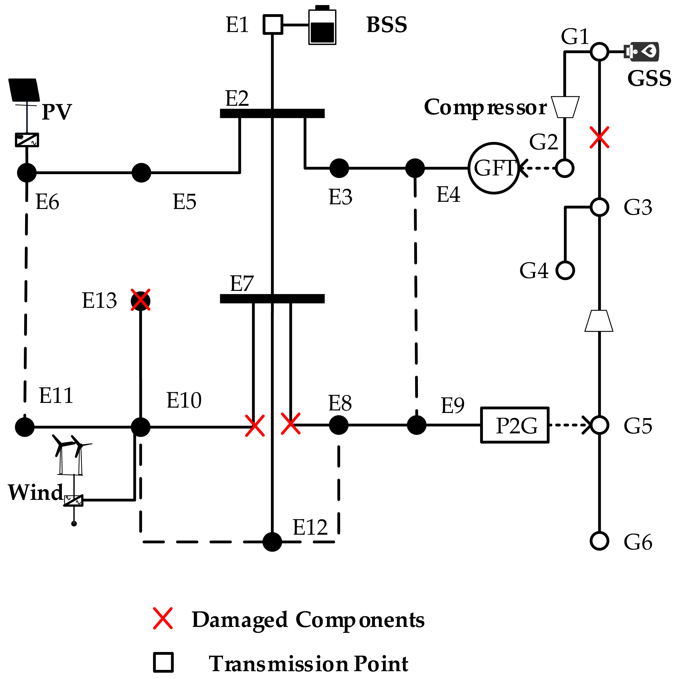
2.1. Introduction to Failure Restoration

First, to emphasize the importance of the temporal characteristics of failure restoration, the several stages that happen when the IEGS suffers from a fault need to be analyzed. Traditionally in an electric power system, failure restoration studies mainly focus on the two-stage failure restoration process, as shown in Figure 1a, including the faulty stage and the restored stage, but in an IEGS, due to the tightly coupled nature, the two-stage failure restoration process cannot represent the temporal characteristics of the topology, DGs, BSS and GSS, which may lead to unfeasible operation results in the restoration process. To this end, this paper applies the three-stage failure restoration process for the IEGS. As shown in Figure 1b, there is one more stage, the failover stage, which includes the dynamic process of topology, the output of DGs, BSS, and GSS. Second, the structure of the IEGS needs to be introduced. The electric network is bidirectionally coupled with the natural gas network through gas-fired turbine (GFT) and power-to-gas (P2G) devices. The energy management system (EMS) of IEGS can achieve the information acquisition and remote dispatching through the remote terminal unit (RTU), and the controllable equipment such as GFT, P2G, BSS, and GSS are dispatched to achieve the reliable and economical operation.

The software function of failure restoration can be integrated into the energy management system of IEGS. After a large-scale outage accident (such as earthquakes, typhoons, and other harsh natural disasters) happens, neither the electric nor gas transmission systems can supply energy to the corresponding distribution systems. At the same time, the electric distribution network and the gas distribution network also suffer inevitable failures. By dispatching the output of GFT, P2G, BSS, GSS, and actions of switchgear in the electric network and the action of the pipeline valves in the natural gas network, the dispatching center can quickly restore the electric power supply and natural gas supply after the large-scale outage happens. Besides, the GFT can transform natural gas into the electricity for supporting the electric network. Conversely, P2G can supply natural gas networks by consuming electricity. Through both approaches, the purpose of maximizing the restored load can be achieved. Figure 2 shows the flowchart of the restoration process.

2.2. Objective of the Failure Restoration Model

In order to simplify the modeling of failure restoration and guarantee the feasibility of the problem, it is necessary to make the following assumptions:

(1)

The topology of the electric network and the natural gas network maintain a radial operation, in which the energy flow is bi-directional;

(2)

The transmission network cannot supply energy to the distributed electric and natural gas network. The IEGS needs to perform a local failure restoration. It is assumed that the IEGS can maintain the islanded operation before the fault is repaired.

(3)

The remote terminal units and the communication networks are not affected by the disaster which means they can operate normally within the restoration process.

The goal of failure restoration is to maximize the interrupted load, including electrical and natural gas loads. It can be formulated by the following mathematical forms:

$$\begin{array}{l}\max {\displaystyle \sum _i{\displaystyle \sum _t{\beta }_i^L·\Delta t·P_{i,t}^D}+}{\displaystyle \sum _n{\displaystyle \sum _t{\beta }_n^L·\Delta t·F_{n,t}^D}},i\in {\Omega }_e,n\in {\Omega }_g,t\in T\\ \mathrm{s}.\mathrm{t}.\mathrm{constraints}\mathrm{of}\mathrm{electric}\mathrm{network}\\ \mathrm{constraints}\mathrm{of}\mathrm{natrual}\mathrm{gas}\mathrm{network}\\ \mathrm{coupling}\mathrm{constraints}\mathrm{of}\mathrm{the}\mathrm{IEGS}\\ \mathrm{constraints}\mathrm{of}\mathrm{topology}\end{array}$$

(1)

where: the electrical load $P_{i,t}^D$ and the natural gas load $F_{n,t}^D$ are multiplied by the coefficients ${\beta }_i^L$ and ${\beta }_n^L$, respectively, representing the priority of different loads. $\Delta t$ indicates the action period of each operation step, one hour is taken [31]. Subscript t denotes serial time. T is the set of time which belongs to the whole restoration period. ${\Omega }_e$ and ${\Omega }_g$ represent the set of nodes in the electric network and natural gas network, respectively.

The above mathematical model is a mixed-integer nonlinear programming problem. In this paper, the nonlinear terms are handled with a linearization method. The constraints in (1) will be described separately in the following sections.

2.3. Modelling of the Electric Network

The linear DistFlow equation has been widely used in the power flow of radial distribution networks and microgrid systems, as shown in Figure 3. The equations are relatively easy to solve because the non-linear terms in the original power flow equation are neglected. Based on the DistFlow equation, this paper introduces the binary variables of each line, and the modified power flow constraints of the electric network are obtained.

For each node in the electric network, the power flowing in and out should be equal:

$${\displaystyle \sum _{ki\in {\Omega }_{\mathrm{l}}^{\mathrm{elc}}}{P}_{ki,t}}+P_{i,t}^{\mathrm{dg}}-{\displaystyle \sum _{ij\in {\Omega }_{\mathrm{l}}^{\mathrm{elc}}}{P}_{ij,t}}=v_{i,t}{P}_{i,t}^{\mathrm{D}},\forall i\in {\Omega }_{\mathrm{e}},t\in T$$

(2)

$${\displaystyle \sum _{ki\in {\Omega }_{\mathrm{l}}^{\mathrm{elc}}}{Q}_{ki,t}}+Q_{i,t}^{\mathrm{dg}}-{\displaystyle \sum _{ij\in {\Omega }_{\mathrm{l}}^{\mathrm{elc}}}{Q}_{ij,t}}=v_{i,t}{Q}_{i,t}^{\mathrm{D}},\forall i\in {\Omega }_{\mathrm{e}},t\in T$$

(3)

where $P_{ki,t}$ represents the active power flow in the line (k,i) which connects the nodes k and i. $P_{i,t}^{\mathrm{dg}}$ is the generated active power of DGs in the node i at time t. $P_{i,t}^{\mathrm{D}}$ denotes the active power consumption in the node i at time t. $v_{i,t}$ stands for the status of restoration in node i at time t, node is restored when $v_{i,t}=1$, otherwise $v_{i,t}=0$. ${\Omega }_{\mathrm{l}}^{\mathrm{elc}}$ denotes the set of lines in the electric network. (3) is the corresponding reactive power equation.

For each line in the electric network, the nodal voltages of both sides have a relationship with the active and reactive power flow of the corresponding line. The restoration status variables are also introduced:

$$V_{i,t}^{}-V_{j,t}^{}=2(P_{ij,t}{R}_{ij}+Q_{ij,t}{X}_{ij})+b_{ij,t},\forall ij\in {\Omega }_{\mathrm{l}}^{\mathrm{elc}},t\in T$$

(4)

$$(x_{ij,t}-1)V_0^{}\le b_{ij,t}\le (1-x_{ij,t})V_0^{},\forall ij\in {\Omega }_{\mathrm{l}}^{\mathrm{elc}},t\in T$$

(5)

where Equation (4) represents the relationship between the voltage drop and the power flow in each line. $V_{i,t}^{}$ denotes the amplitude of voltage in node i. $R_{ij}$, $X_{ij}$ are the resistance, reactance of line (i,j), respectively. $x_{ij,t}$ represents the restoration status of line (i,j). $b_{ij,t}$ is the auxiliary variable of line (i,j). When the line (i,j) is energized, $x_{ij,t}$ = 1 From the constraint (5) we know the corresponding $b_{ij,t}$ = 0, thus the voltage equation (4) is feasible. On the contrary, when the line (i,j) is de-energized $x_{ij,t}$ = 0, $b_{ij,t}\in [-V_0,V_0]$, $V_0$ is the base voltage.

For each line in the electric network, there is a capacity limit:

$$-P_{ij}^{\max }{x}_{ij,t}\le P_{ij,t}\le P_{ij}^{\max }{x}_{ij,t},\forall ij\in {\Omega }_{\mathrm{l}}^{\mathrm{elc}},t\in T$$

(6)

$$-Q_{ij}^{\max }{x}_{ij,t}\le Q_{ij,t}\le Q_{ij}^{\max }{x}_{ij,t},\forall ij\in {\Omega }_{\mathrm{l}}^{\mathrm{elc}},t\in T$$

(7)

where $P_{ij}^{\max }$ is the limit of active power flow in the line (i,j). The sign of negative and positive denotes the bi-direction of power flow. When line (i,j) is energized, $x_{ij,t}$ = 1, the capacity constraints of lines are active. Otherwise, the power flow of lines is zero. (7) is the corresponding reactive constraint of line (i,j).

For each nodal bus in the electric network, there is a voltage limit:

$$V^{\min }\le V_{i,t}\le V^{\max },\forall i\in {\Omega }_{\mathrm{e}},t\in T$$

(8)

where $V^{\min }$, $V^{\max }$ are the minimum and maximum limit of the voltage of each node. 0.9 and 1.1 are taken, respectively [43].

A battery storage system (BSS) can assist in handling the intermittent problem of DGs and load demands which has an inter-temporal dispatching requirement. The main concern of BSS dispatching is to control the power of charging or discharging, and the remaining SOC. The mathematical model of the BSS adopted in this paper does not consider the specific battery model and parameters, but only the general modeling, the mathematical form is as follows:

$$0\le P_{\mathrm{bss},t}^{\mathrm{c}}\le {\alpha }_{\mathrm{c}}{P}_{\mathrm{bss}}^{\max },\forall t\in T$$

(9)

$$0\le P_{\mathrm{bss},t}^{\mathrm{d}}\le {\alpha }_{\mathrm{d}}{P}_{\mathrm{bss}}^{\max },\forall t\in T$$

(10)

$${\alpha }_{\mathrm{c}}+{\alpha }_{\mathrm{d}}\le 1;{\alpha }_{\mathrm{c}},{\alpha }_{\mathrm{d}}\in \{0,1\}$$

(11)

$${\phi }_{\min }\le {\phi }_t^{\mathrm{bss}}\le {\phi }_{\max },\forall t\in T$$

(12)

$${\phi }_t^{\mathrm{bss}}={\phi }_{t-1}^{\mathrm{bss}}+{\eta }_{\mathrm{c}}^{}{P}_{\mathrm{bss},t-1}^{\mathrm{c}}\Delta t-{\eta }_d^{-1}{P}_{\mathrm{bss},t-1}^{\mathrm{d}}\Delta t,\forall t\in T$$

(13)

where α_c, α_d are the charging and discharging status variable of BSS, respectively. α_c = 1, α_d = 1 indicates that the BSS is in charging and discharging, respectively. $P_{\mathrm{bss},t}^{\mathrm{c}}$, $P_{\mathrm{bss},t}^{\mathrm{d}}$ denotes the active power of charging and discharging, respectively. ${\phi }_t^{\mathrm{bss}}$ is the status of charging of BSS at time t. η_c, η_d are the efficiency of charging and discharging, respectively. For simplicity, it is assumed that the efficiency is not affected by the charging power. Besides, enough reactive capacity is assumed.

2.4. Modelling of the Natural Gas Network

The natural gas network comprises a gas source, pipelines, compressor, storage and load (Figure 4). For simplicity, the steady natural gas flow formulation is utilized, the pipeline storage and dynamic characters are ignored [44].

Meanwhile, the radial operation topology is assumed. With these assumptions, the constraints of nodal balance and pipeline flow in a natural gas network could be formulated as follows:

$${\displaystyle \sum _{ki\in {\Omega }_{\mathrm{l}}^{\mathrm{gas}}}{F}_{ki,t}}+F_{i,t}^{\mathrm{P}2\mathrm{G}}-{\displaystyle \sum _{ij\in {\Omega }_{\mathrm{l}}^{\mathrm{gas}}}{F}_{ij,t}}=v_{i,t}{F}_{i,t}^{\mathrm{D}}+F_{i,t}^{\mathrm{GFT}},\forall i\in {\Omega }_{\mathrm{g}},t\in T$$

(14)

where $F_{ki,t}$ represents the gas flow of pipeline (k,i) at time t. $F_{i,t}^{\mathrm{D}}$ is the gas consumption of node i at time t. $F_{i,t}^{\mathrm{P}2\mathrm{G}}$ stands for the output amount of gas of P2G. $F_{i,t}^{\mathrm{P}2\mathrm{G}}$ stands for the gas consumption of GFT. ${\Omega }_{\mathrm{l}}^{\mathrm{gas}}$ is the set of pipelines in the natural gas network, ${\Omega }_{\mathrm{g}}$ is the set of nodes in the natural gas network.

The natural gas pipelines can be divided into two categories: pipelines with compressors and pipelines without compressors. For the pipelines with compressors, the gas flow constraints can be expressed as follows:

$${\pi }_{i,t}\le {\pi }_{j,t}\le {\lambda }_{ij}{\pi }_{i,t},\forall ij\in {\Omega }_{\mathrm{l}}^{\mathrm{gas}},t\in T$$

(15)

$$0\le F_{ij,t}\le F_{ij,t}{x}_{ij,t},\forall ij\in {\Omega }_{\mathrm{l}}^{\mathrm{gas}},t\in T$$

(16)

where ${\pi }_{i,t}$ represents the pressure of node i at time t. $x_{ij,t}$ is the binary variable, representing the status of restoration in the pipeline (i,j). The pipeline is restored when $x_{ij,t}=1$, otherwise $x_{ij,t}=0$. ${\lambda }_{ij}$ is the parameter of the compressor in the pipeline (i,j), corresponding to different operating conditions. The compressor could be illustrated as Figure 5, energy consumption of compressor is ignored just for simplification.

At the same time, for natural gas pipelines without compressors, the gas flow has the following relationship with node pressure:

$${\mathrm{sgn}}_{ij,t}({\pi }_{i,t}^{},{\pi }_{j,t}^{})F_{ij,t}^2={\Phi }^2\left({\pi }_{i,t}^2-{\pi }_{j,t}^2\right),\forall ij\in {\Omega }_{\mathrm{l}}^{\mathrm{gas}},t\in T$$

(17)

$${\mathrm{sgn}}_{ij,t}({\pi }_{i,t}^{},{\pi }_{j,t}^{})=\left\{\begin{array}{l}+1,{\pi }_{i,t}^{}>{\pi }_{j,t}^{}\\ -1,{\pi }_{i,t}^{}<{\pi }_{j,t}^{}\end{array}\right.$$

(18)

where $\Phi$ indicates the comprehensive parameter of the pipeline [45]. ${\mathrm{sgn}}_{ij,t}({\pi }_{i,t}^{},{\pi }_{j,t}^{})$ represents the direction of the gas flow in the pipelines. Because of the existence of quadratic terms in the Equation (17), there is a need to eliminate these nonlinear terms. Squaring both sides of (17), letting ${\mu }_{i,t}={\pi }_{i,t}^2$. Then the auxiliary variables δ, $\eta$ are introduced to do the incremental linearization [46,47]:

$$\begin{array}{ll}{\mathrm{sgn}}_{ij,t}({\pi }_{i,t}^{},{\pi }_{j,t}^{})F_{ij,t}^2& =F_{ij,t,1}^2+{\displaystyle \sum _{k=1}^N[(F_{ij,t,k+1}^2)-(F_{ij,t,k}^2)]}·{\delta }_k\\ & ={\Phi }^2({\mu }_{i,t}-{\mu }_{j,t}),\forall ij\in {\Omega }_l^{gas},t\in T\end{array}$$

(19)

$$\begin{gathered} F_{ij,t}=F_{ij,t,1}+{\displaystyle \sum _{k=1}^N[(F_{ij,t,k+1}^{})-(F_{ij,t,k}^{})]}·{\delta }_k \\ \forall ij\in {\Omega }_{\mathrm{l}}^{\mathrm{gas}},t\in T \end{gathered}$$

(20)

$$\left\{\begin{array}{l}{\delta }_{k+1}\le {\eta }_k\le {\delta }_k,k=1,2,...,N-1\\ 0\le {\delta }_k\le 1,{\eta }_k\in \{0,1\},k=1,2,...,N\end{array}\right.$$

(21)

Equation (19) is a piecewise linear form of a square function, (20) is a piecewise linear form of independent variables. Equation (21) are constraints of the introduced variable corresponding to piecewise positions and quantities, k is piecewise number, and N is the total piecewise quantities. After applied with the above incremental linearization, the non-linear term in the (17) can be eliminated.

The GSS can provide standby natural gas supply after system failure to support short-term failure restoration. Similar to BSS, the model of GSS can be formulated as follows:

$$S_{i,t}=S_{i,t-1}+(F_{i,t-1}^{\mathrm{in}}-F_{i,t-1}^{\mathrm{out}})·\Delta t,\forall i\in {\Omega }_{\mathrm{g}},t\in T$$

(22)

$$S_i^{\min }\le S_{i,t}\le S_i^{\max },\forall i\in {\Omega }_{\mathrm{g}},t\in T$$

(23)

$$0\le F_{i,t}^{\mathrm{in}}\le F_{i,t}^{\mathrm{in},\max },\forall i\in {\Omega }_{\mathrm{g}},t\in T$$

(24)

$$0\le F_{i,t}^{\mathrm{out}}\le F_{i,t}^{\mathrm{out},\max },\forall i\in {\Omega }_{\mathrm{g}},t\in T$$

(25)

where $S_{i,t}$ indicates the remaining gas capacity of GSS in node i at time t. $S_i^{\min }$, $S_i^{\max }$ represent the minimum and maximum gas capacity limit of GSS, respectively. $F_{i,t}^{\mathrm{in}}$, $F_{i,t}^{\mathrm{out}}$ indicate the input and output gas flow of GSS in node i at time t.

The nodal pressure of natural gas network needs to be within a reasonable range in order to ensure safe operation. The corresponding constraints are as follows:

$${\pi }^{\min }\le {\pi }_{i,t}\le {\pi }^{\max },\forall i\in {\Omega }_{\mathrm{g}},t\in T$$

(26)

where ${\pi }^{\min }$,${\pi }^{\max }$ are the minimum and maximum limit of pressure in the natural gas network, respectively.

IEGS achieves bi-directional coupling through GFT and P2G. By opening the P2G device, surplus electricity can be converted into natural gas and injected into the natural gas network for storage and transportation. The GFT can consume the natural gas for generating the electricity into the electric network:

$$F_{i,t}^{\mathrm{GFT}}=\frac{P_{i,t}^{\mathrm{GFT}}}{{\eta }_i^{\mathrm{GFT}}G},i\in {\Omega }_{\mathrm{GFTU}}$$

(27)

where $F_{i,t}^{\mathrm{GFT}}$ represents the gas consumption of GFT in node i at time t. $P_{i,t}^{\mathrm{GFT}}$ is the output active power of GFT in node i at time t. $G$ represents the low calorific value of natural gas (35590 kJ/m³) is taken from [48]. ${\Omega }_{\mathrm{GFTU}}$ denotes the set of GFT units.

$$F_{i,t}^{\mathrm{P}2\mathrm{G}}=\frac{{\eta }_i^{\mathrm{P}2\mathrm{G}}·P_{i,t}^{\mathrm{P}2\mathrm{G}}}{G},i\in {\Omega }_{\mathrm{P}2\mathrm{GU}}$$

(28)

where $F_{i,t}^{P2G}$ represents the output natural gas of P2G in node i at time t. $P_{i,t}^{P2G}$ is the active power consumption of P2G in node i at time t. ${\Omega }_{\mathrm{P}2\mathrm{GU}}$ denotes the set of P2G units.

2.5. Topology Constraints

In the whole process of failure restoration, the electric network involves the operation sequence of line switches, load switches, BSS, etc. The natural gas network involves the operation sequence of pipeline valves, GFT and P2G. Topology constraints ensure that the IEGS can maintain the radial topology in each step of the entire failure restoration. It should be emphasized that the essential difference between the reconfiguration and failure restoration problem modeling is how to formulate the radial constraints. There are a considerable number of studies about distribution network reconfiguration, the explanation of which is given here to make this paper self-contained. The reconfiguration of a distribution network is essentially a minimum spanning tree problem with an objective of loss-reduction. Generally, the single substation node scenario is considered in the reconfiguration problem. Thus, to ensure the radial topology after the completion of reconfiguration, the following concise constraint could be adopted to the model:

$${\displaystyle \sum _{ij\in {\Omega }_l^{elc}}{x}_{ij}}=\left|{\Omega }_e\right|-1$$

(29)

Equation (29) can be interpreted in the following logic. The topology graph consists of vertexes and edges. The sufficient and necessary condition of radial graph is that the number of vertexes equals the number of vertexes minus one. The number one on the right-hand side of (29) indicates the number of substations (i.e., root node). Figure 6 shows a possible reconfiguration process in which the constraint (29) always holds. The operation nature restricts that the topology must be radial, i.e., it must be a single spanning tree. However, things change in the failure restoration case. Because there are potentially two kinds of nodes after the change of topology completed, i.e., energized nodes and non-energized nodes which can form multiple not-connected subgraphs. In this case, we call this subgraph a spanning forest consisting of multiple spanning trees. We will give a simple example to demonstrate this case in Figure 7. The branch S1 is assumed to be faulty, the downstream area, including nodes 2,4,5 is de-energized. After the service restoration is executed, the tie-branch S7 is closed, branch S4 is open. Thus, the original graph is divided into two parts, i.e., two spanning trees. In this case, the value of left-hand side of (29) is 5, but the right-hand side equals to 6. It is obvious that (29) is valid to make topology radial only when the second term of right-hand side equals to the numbers of formed trees, in Figure 7 this number is 2. However, we cannot be aware of how many trees will be formed in advance. Therefore, the radial constraint (29) in reconfiguration cannot be applied to the failure restoration straightly.

In this paper, we will introduce new radial constraints for the failure restoration. Since we do not know the exact numbers of the possible trees that would be formed, the idea is to connect all the remaining trees except for the restored part. Thus, the fictitious node is introduced to be the root node of the de-energized area, the fictitious branches connecting the real load nodes and fictitious node are generated correspondingly. In this way, there will always be two trees after the failure restoration executed. The following mathematical constraints are introduced:

$${\displaystyle \sum _{ki\in {\Omega }_{lf}}{H}_{ki}}-{\displaystyle \sum _{ij\in {\Omega }_{lf}}{H}_{ij}}+H_i^{Gf}=H_i^{Df}(1-y_i),\forall i\in {\Omega }_e\cup N_f$$

(30)

$$0\le H_{ij}\le x_{ij},\forall ij\in {\Omega }_{lf}$$

(31)

$$H_i^{Gf}=0,\forall i\in {\Omega }_e$$

(32)

${\Omega }_{lf}$ is the set of fictitious branch. $H_{ij}$ is the fictitious flow of branch (i,j). $H_i^{Gf}$, $H_i^{Df}$ are fictitious generation and demand in node i, respectively. Each de-energized node (i.e., those y_i equals 0) requires a little fictitious load demand, and only the fictitious node N_f supplies the fictitious generation. Thus, Equation (30) ensures that each de-energized node connects the fictitious root node N_f. After applying these constraints, the graph after the failure restoration is a 2-tree, the original minimum spanning forest problem has been transformed into a 2-tree spanning problem. Back to Equation (29), since we already know there must be two trees after the failure restoration, the corresponding radial constraint could be modified into following form:

$${\displaystyle \sum _{ij\in {\Omega }_l^{elc}\cup {\Omega }_{lf}}{x}_{ij}}=\left|{\Omega }_e\cup N_f\right|-2$$

(33)

However, there is another situation we should take into consideration which the existing studies have not mentioned before. That is, the de-energized node can potentially be contained in the energized tree. The reason is that the load priority w_i has been included in the objective function. In general, if we do not account for w_i, the failure restoration would restore the loads which have a shorter path to the substation node. Because the shorter path has less possibility to violate the voltage and capacity constraints. Figure 8b shows this common situation in which the nodes 2,4 could not get restored while node five get energized again. However, if taking the load priority into consideration, let’s assume that node 2 has a higher priority than node 5 (i.e., w₂ > w₅), the restored topology could be the Figure 8c in which the de-energized node 5 is included into the energized area, the corresponding Equation (33) is not valid, the left-hand side of which is 7 while the right-hand side is 6.

Furthermore, we will introduce another indicator variable to exclude the above invalidity. Intuitively, if we know the number of nodes which are de-energized nodes embodied in the energized area, then Equation (33) can be modified to valid. These nodes have an obvious characteristic that they have at least one child node which has a status of being restored. In Figure 8c, the child node of 5 is node 2 which is restored. Therefore, we can exclude these nodes from the connection with the fictitious network by force the corresponding fictitious branch to be open (branch N_f-5 in Figure 8c). In this way, (33) can be valid. The general mathematical formulation of above analysis can be represented by the following logical constraints:

If a node has at least one restored node, i.e.,

$${\displaystyle \sum _{jk\in {\Omega }_l^{elc}}{x}_{jk}{y}_k}\ge 1,\forall ij\in {\Omega }_{lf}$$

(34)

Then the fictitious branch which connects that node should be open, i.e., x_ij = 0.

If a node does not have restored node, i.e.,

$${\displaystyle \sum _{jk\in {\Omega }_l^{elc}}{x}_{jk}{y}_k}=0,\forall ij\in {\Omega }_{lf}$$

(35)

Then the fictitious branch which connects that node could be open or closed, i.e., x_ij is binary.

We then combine the above logical constraints to the following compact linear form:

$${\displaystyle \sum _{jk\in {\Omega }_l^{elc}}{x}_{jk}{y}_k}-1\le M(1-x_{ij}),\forall ij\in {\Omega }_{lf}$$

(36)

The parameter M in (36) has a similar idea as the Big-M method, but in this case the M represents the maximum numbers of children nodes of one specific node. Now, we have finished the processing of radial constraints in failure restoration. Then, we can obtain the deterministic failure restoration model which consists of objective function (1), operation constraints (2)–(28), fictitious network constraints (30)–(32), and radial constraints (33)(36).

3. Robust Model Formulation

Wind turbines and photovoltaic systems are uncontrollable distributed generations, and their outputs have substantial uncertainty. Meanwhile, the load demands change all the time. Despite the fact there are many studies on methods for forecasting the output of distributed generations and load demands, errors in forecasting are unavoidable. The focus of this paper is not on the method of forecasting, but is based on the assumption that the forecasting range of distributed generations and load demands have been obtained. Based on this, the uncertainty set in the form of a box is used to describe the forecasted error:

$$P_{i,t}^{dg}=P_{i,t}^{dg}{}^{\ast }-g_i{\tilde{P}}_i,\forall i\in {\Omega }_{\mathrm{e}},t\in T$$

(37)

$$P_{i,t}^D=P_{i,t}^D{}^{\ast }-g_i{\tilde{P}}_i,\forall i\in {\Omega }_{\mathrm{e}},t\in T$$

(38)

$${\displaystyle \sum _{i\in {\Omega }_e}{g}_i}\le \tau$$

(39)

$$g_i\in [0,1],\forall i\in {\Omega }_{\mathrm{e}}$$

(40)

where: ${\tilde{P}}_i$ is the forecasted error. $g_i$ is the uncertainty coefficient. (39) represents the set of uncertainty in robust optimization theory. The value of τ is called the uncertainty budget. The conservativeness of the robust model can be controlled by adjusting the value of τ. When τ = 0, the uncertainty set is empty, and the robust model degenerates into the traditional deterministic model. When τ = |Ω_e|, the uncertainty set is the largest corresponding to the worst scenario which means the maximum deviation from the forecasted value. By choosing the appropriate uncertainty budget τ, the extreme cases can be avoided.

With the uncertainty has been modeled, the robust failure restoration model can be formulated as the following three-layer mixed-integer linear programming form:

$$\underset{x}{\max }\underset{p}{\min }\underset{y\in F(x,p)}{\max }{c}^{\mathrm{T}}y$$

(41)

$$\mathrm{s}.\mathrm{t}.Ay\le b$$

(42)

$$Cy+Dx\le f$$

(43)

where $x:=(x_{ij},y_i)$ $p:=(P_i^D,P_i^{dg})$ $y:=(P_{ij},Q_{ij},V_i^{},F_{ij},{\pi }_i)$.

$F(x,p)$ in (41) indicates the relationship between topology and energy flow, Equation (42) is the topology constraints. The electric and natural gas flow constraints and remaining operation constraints are represented by inequalities (43). A, C, D, b, f are the constant matrix or vector related to the corresponding constraint.

The first-layer determines the sequential topology and switch actions. For the uncertainty, the min problem of the second-layer looks for the worst operating scenario in which the minimal restored load demands would be achieved. The third-layer aims to find the optimal dispatching strategy to recover load demands as much as possible.

The three-layer robust optimization problem is difficult to solve directly. For such a problem, the C&CG algorithm [42] and the benders decomposition algorithm [49] are often adopted. Both algorithms use an iterative framework which decomposes the original problem into two sub-problems. The difference is that the original tangent planes and generated variables are added to the main problem in the C&CG algorithm. Thus, the number of iterations is significantly reduced compared to the benders decomposition method. Therefore, this paper uses C&CG algorithm to solve (41)–(43).

4. Case Study

In this section, an IEGS composed of a 13-node electric network and a 6-node natural gas network is utilized as a case study to verify the effectiveness of the proposed method. The simulation environment is under MATLAB. The optimization problem is modeled by YALMIP [50] and solved by CPLEX [51].

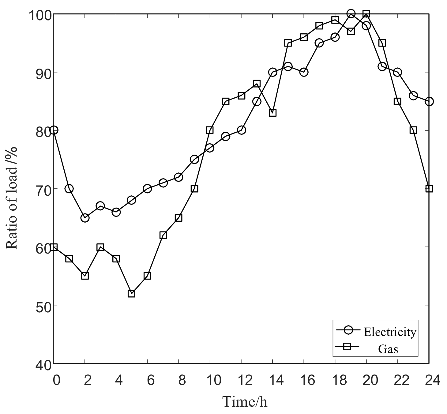
4.1. Simulation Parameters

The topology of the IEGS is shown in Figure 9. In order to distinguish the different nodes of two networks, the letters G and E are used to represent natural gas and electric nodes, respectively. Moreover, the brackets are used to represent lines and pipelines. The dotted lines represent the tie-lines which are open under normal condition. Two networks are coupled by one GFT at node E4 and one P2G at node E9. The original three-phase unbalanced IEEE 13-node distribution network [52] has been modified into a balanced network. The line parameters of IEEE 13-node distribution network are shown in

Table 1. Lines parameters of IEEE 13-node network.

Line Index	Starting Node	Ending Node	Length (ft)	Capacity (kVA)
1	1	2	2000	1500
2	2	3	500	1000
3	3	4	200	500
4	2	5	500	1000
5	5	6	300	800
6	2	7	2000	1500
7	7	8	10	800
8	8	9	500	800
9	7	10	300	800
10	10	11	300	800
11	10	12	300	800
12	7	12	1000	1500
13	6	11	2000	800
14	8	12	1500	1000
15	4	9	600	700

, and the base electric loads are shown in

Table 2. Base electric loads.

Node Index	Active Load (kW)	Reactive Load (kVar)	Weight Coefficient
2	100	40	2.12
4	100	40	1.44
5	200	100	1.14
6	200	100	3.29
7	300	180	2.66
8	200	150	2.90
9	200	40	2.88
11	200	120	1.66
12	200	120	1.68
13	40	30	1.84

, which will fluctuate by percentage over time, as shown in Figure 10. The weight coefficients are randomly generated from 1 to 5 with a uniform distribution which could be modified by the operators on the basis of real-life condition. The pipeline parameters of the natural gas network are shown in

Table 3. Pipeline parameters of the natural gas network.

Pipeline Index	Starting Node	Ending Node	Parameter
1	1	2	1.095
2	1	3	1.095
3	3	4	1.173
4	3	5	1.158
5	5	6	1.158

, the loads data of the natural gas network is shown in

Table 4. Loads data of the natural gas network.

Load Index	Gas Load (Sm3/h)	Upper Limit of Pressure (bar)	Lower Limit of Pressure (bar)	Weight Coefficient
1	29.8	75	20	5.82 0.4610 2.8390 2.7997 1.4197 2.3408
2	10.4	60	20	5.46
3	12.6	60	20	4.83
4	16.5	60	20	7.79
5	11.0	60	20	6.41
6	11.6	60	20	5.34

. There are two compressors in the pipeline (G3, G5) and (G1, G2),

Table 5. Compressor parameters of natural gas network.

Compressor Index	Starting Node	Ending Node	Lower Limit of Ratio	Upper Limit of Ratio
1	G1	G2	1.0	1.3
2	G5	G3	1.0	1.2

shows the parameters. The specific parameters of these two devices are shown in

Table 6. Parameters of coupling devices.

	Electric Node	Gas Node	Upper Limit of Active Power (kW)	Efficiency
GFT	E4	G2	800	0.43
P2G	E9	G5	300	0.62

. Two energy storage devices are embedded in the system,

Table 7. Parameters of energy storage devices.

	Node	Initial Capacity	Limit of Capacity	Limit of Charging Rate	Limit of Discharging Rate
BSS	E1	2500 kWh	3000 kWh (kw)	750 kW/h	750 kW/h
GSS	G1	800 m3	300 m3	100 m3/h	100 m3/h

shows the specific parameters.

Assuming that a failure occurs at time 12:00, the transmission network cannot supply energy to the electric network and the natural gas network, two lines in the electric network (E7, E10) and (E7, E8) are broken, and pipeline (G1, G3) is broken, the electric load E13 is damaged. In order to provide short-term failure restoration, it is necessary to dispatch the local energy devices in the IEGS. For this purpose, three cases are designed to verify the effectiveness of the proposed method.

Case1: Without considering the coupling, the failure restoration of electric network and natural gas network are carried out independently;

Case2: Considering one-way coupling, only the GFT in the system is dispatched;

Case3: Considering two-way coupling, the GFT and P2G are dispatched simultaneously.

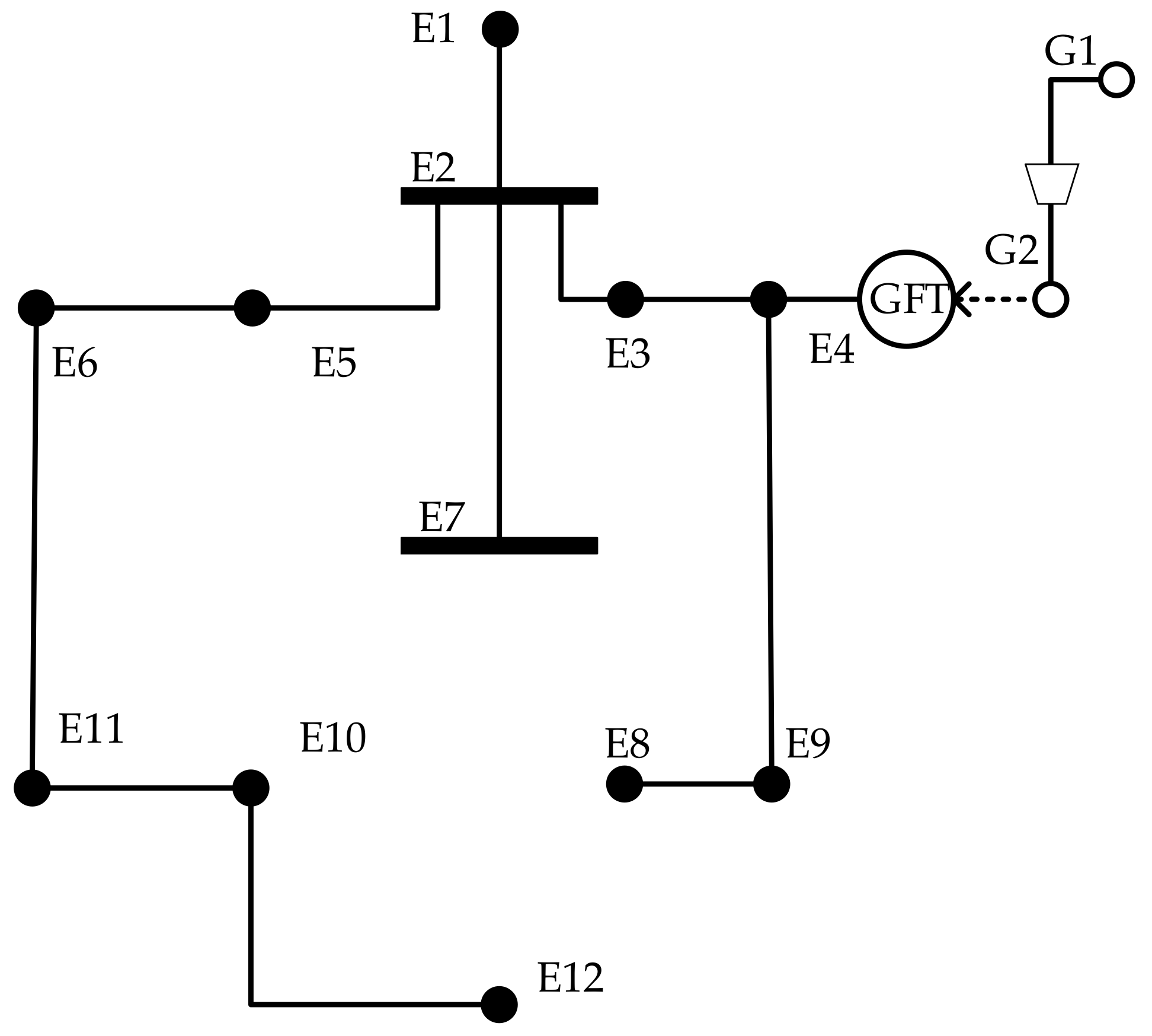
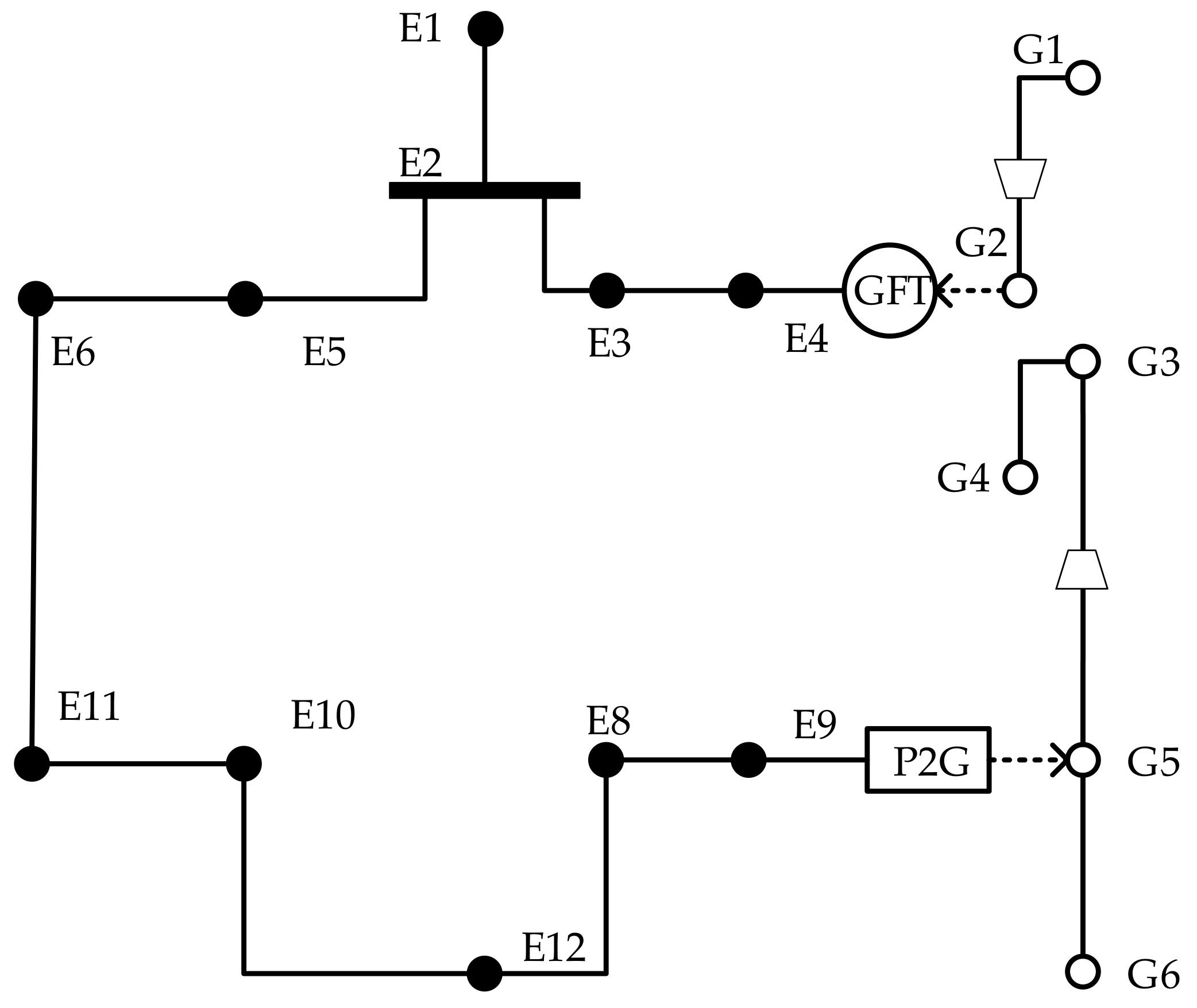
4.2. Failure Restoration Process Analysis

Firstly, the objective function value (i.e., total restored load with a weighted coefficient, including electric and natural gas load) are compared in the three cases. As shown in

Table 8. Objective function value in the three cases.

Case	Objective Function Value	Electricity Part	Natural Gas Part	Computational Time (s)
1	22113.58	17743.85	4369.73	1.022
2	34469.85	30100.12	4369.73	1.076
3	39874.69	20489.57	19385.12	2.195

, the objective value of three cases increase in turn, and the computation time is about 1 second. For Case 1, the excess natural gas in the GSS cannot be converted into electricity because of the lack of existence of an electricity-gas coupling device, so the downstream of the failed pipeline gets no energy supply. Thus, the total restored load is relatively low, just only 55.51% of Case 3. For Case 2, only the GFT coupling is considered, and the excess natural gas can be transformed into electricity, resulting in a higher restored electric load compared to Case 1. However, the downstream of the failure pipeline in the natural gas network cannot be restored either, so the natural gas parts in Case 1 and 2 are the same. The objective function value of Case 2 is about 86.45% of Case 3. However, due to the failure to restore the natural gas load, the electric load is higher than Case 3. In Case 3, the extra electricity generated by the photovoltaic system can be converted into natural gas by the P2G, thus further restoring the natural gas load. Among the three cases, Case 3 has the maximum objective function value 39,874.69, which means that the maximum electric and gas loads are restored, the effectiveness of the proposed two-way coupling failure restoration is demonstrated.

Secondly, the restoration process in each case would be analyzed in detail. The restoration actions of lines/pipelines and load in three cases are shown in

Table 9. Restoration actions of the three cases.

Step	Restored Lines			Restored Loads
	Case 1	Case 2	Case 3	Case 1	Case 2	Case 3
1	-	-	-	G1	G1	G1
2	(G1,G2),(E1,E2)	(G1,G2),(E1,E2)	(G1,G2),(E1,E2)	G2,E2	G2,E2	G2,E2
3	(E2,E5)	(E2,E3),(E2,E5)	(E2,E3),(E2,E5)	E5	E5	-
4	(E5,E6)	(E3,E4),(E5,E6)	(E3,E4),(E5,E6)	E6	E4,E6,GFT	E4,E6,GFT
5	(E6,E11)	(E4,E9),(E6,E11)	(E6,E11)	E11	E9,E11	E11
6	(E11,E10)	(E2,E7)	(E11,E10)	-	E7	E10
7	(E10,E12)	(E9,E8),(E11,E10)	(E10,E12)	E12	E8,E10	E12
8	(E12,E8)	(E10,E12)	(E12,E8),(E8,E9)	E8	E12	E8
9	-	-	P2G	-	-	G5
10	-	-	(G5, G3),(G5,G6)	-	-	G3,G6
11	-	-	(G3,G4)	-	-	G4

. In each step of the restoration process, all constraints in (1) need to be satisfied. In Case 3, compared with Case 1 and Case 2, six extra loads (electric load: E4, E9; gas load: G3, G4, G5, G6) and four loads (gas load: G3, G4, G5, G6) are restored, respectively.

In Case 1, because no extra natural gas is transformed into electricity, the load in the electric network is entirely supplied by the BSS and DG. Thus, the DG located at node E6 and E10 are restored first, the downstream load E8 and E12 are restored through closing the tie-lines (E6, E11), (E12, E8) as shown in Figure 11. To emphasis the change of topology, DGs and BSS, ESS are not drawn in the figure.

In Case 2, due to the existence of GFT at node E4, the electricity it generates which assists the restoration of the electric network. The downstream nodes E9 and E8 are restored through closing the tie-line (E4, E9). Meanwhile, because of the local electricity injection at node E4, the output of BSS at node E1 is reduced, and the extra load E7 is restored. Besides, with the support of DG at node E6 and E10, all electric loads are restored. The restored topology is shown in Figure 12.

In the restoration process of Case 3, the natural gas loads can be restored because the electricity can be transformed into natural gas through the P2G at node E9, as shown in Figure 13. The restoration path includes DG at nodes E6 and E10 so that the clean energy generated by them could be transferred to natural gas through P2G. However, due to the long restoration path, the excessive load will lead to the nodal voltage violating the constraints, so the electric load at E5 and E7 would not be restored. Although the amount of restored electric load is less than Case 2, the total restored load in Case 3 is higher than Case 2 because of the extra restoration of the natural gas load.

Through the co-operation of line switch actions, BSS, GSS, P2G and GFT, the restoration process of Case 3 achieves the multi-period failure restoration of the IEGS the maximum interrupted loads are restored, and also the clean energy’s penetration is promoted. This process embodies the complementary advantages of IEGS which increase the reliability of energy supply.

The BSS and coupling devices play a key role in the process of failure restoration. Figure 14 shows the active output of BSS, GFT and the active power consumption of P2G. In general, with the temporal change of the network topology and load, the output of coupling devices changes in real-time in order to make the operation constraints hold. In the fourth and seventh step of the restoration process, DGs are connected to the grid to generate electricity, resulting in the reduction of the output of BSS. The third and eighth step corresponds to the restart-up of GFT and P2G, respectively.

4.3. Comparison of Different Radial Topology Constraints

In order to verify the effectiveness of the proposed radial topology constraints, we design another test to compare the existed modeling method with our model. Assuming there is a fault happens at the line (E2, E7), the topology of the 13-node distribution network has been represented by the graph consisting of vertexes and edges, as shown in Figure 15. For highlighting the superiority of the proposed radial topology constraints, we will focus on the electric distribution network, and the natural gas network is ignored in this test. Once the fault detection and isolation accomplished, the de-energized area can be identified which is set of load buses including E7, E8, E9, E10, E11, E12, E13 in Figure 15. Then, the two restoration modeling methods are applied to recover the interrupted loads.

Figure 16 shows the restoration results using the traditional radial topology constraints [52] modeling method, the load buses E8, E9, E10, E11, E13 get restored. The E7 and E12 do not get restored because the radial topology constraints enforce that there must be two trees after the restoration. Then, we utilize the radial topology constraints proposed in this paper to make the simulation, the restoration results have a better performance on the amount of restored load demands which is 24.9% more than modeling method in [53]. As shown in Figure 17, the restored loads include E7, E8, E10, E12, E13, the unrestored loads are E9 and E11. The reason for getting the different restoration results is that the proposed radial topology constraints allow the formation of flexible trees after the restoration.

In this case, only one tree is formed, the E11 and E9 are shed other than E7 and E12 because of higher priority coefficient of the loads which makes the better restoration results.

4.4. Comparison of Deterministic and Robust Model

Then, in order to prove the effectiveness of the proposed method under uncertainty, Case 4 is designed for simulation. In Case 4, the worst scenario of uncertainty is considered. Meanwhile, the deterministic model of failure restoration is utilized. As shown in

Table 10. The restoration results under normal and worst scenario with deterministic model.

	Case 3 (Normal)	Case 4 (Worst)
Objective function	39874.69	36698.21
Restored electrical nodes	E2,E4,E6,E8,E9,E11,E12	E2,E4,E6,E8, E11
Restored gas nodes	G1,G2,G3,G4,G5,G6	G1,G2,G3,G5,G6

, the objective function value of Case 4 is 92.03% of Case 3 which means that the deterministic model affected by the uncertainty. There is a need to shed more load under the worst scenario which cause the less objective function value, i.e., the restored energy demands, including the electrical and gas loads.

Table 11. Results of restoration under different DGs penetration.

DGs Penetration	Total Restored Loads	Restored Electric Loads	Restored Gas Loads
Low Level	41365.68	25893.88	15471.8
Base Level	39874.69	20489.57	19385.12
High Level	37689.75	15987.69	21702.06

illustrates the restoration results under different DGs penetration. We can observe that with the increase of the DGs penetration, the total restored loads get reduced which means the more loads are shed. The reason behind this is that the proposed model is based on robust optimization, the uncertainty has a great impact on the restoration results. The robust model makes all the restoration solutions feasible under the worst scenario of the uncertainty, thus it needs to shed more loads to handle the potential variation of the DGs’ output.

Meanwhile, we further carry out a test to compare the results obtained by the deterministic model and the proposed robust model under normal uncertain scenarios. We randomly generate 2000 fluctuation scenarios of the uncertain output of DGs using the Monte Carlo sampling method. The restoration results are presented in

Table 12. Results of restoration using Monte Carlo sampling.

Model	Success Rate	Average Restored Power
Deterministic Model	73.5%	36587.68
Robust Model	100%	40256.48

. The success rate represents the portion of scenarios in which the restoration results do not violate the nodal voltage or line capacity constraints. It can be seen that the proposed robust model can get a valid restoration solution in all scenarios. Moreover, the average restored power of robust model is greater than the deterministic model. Thus, the proposed robust model has a superiority than the deterministic model under the condition of uncertainty.

5. Conclusions

Most of the existing research on failure-related aspects of integrated electricity-gas systems focuses on failure prevention and reliability assessment. From the post-failure perspective, this paper proposes a multi-period failure restoration method considering two-way coupling for IEGS. The problem is formulated as a mixed-integer linear programming model, utilizing linearization technology and linear Distflow equations. On the one hand, the proposed failure restoration strategy considering the bidirectional coupling of the electric and natural gas networks has the best result compared to other kinds of coupling; on the other hand, the proposed failure restoration strategy could coordinate the sequential actions of switchgear, BSS, GSS, GFT, and P2G, guaranteeing the safe operation during the whole failure restoration process. The proposed radial topology constraints modeling method can get a better restoration result than the traditional modeling method. Besides, the case study shows that the robust model can handle the uncertainty problem, leading to a more reliable restoration result than the deterministic model. Based on this paper, follow-up works can focus on dynamic natural gas network modeling, and heating network coupling.

References

1. Widl, E.; Tobias, J.; Daniel, S.; Sebastien, N.; Daniele, B.; Sawsan, H.; Tae-Gil, N.; Olatz, T.; Anett, S.; Hans, A. Studying the potential of multi-carrier energy distribution grids: A holistic approach. Energy 2018, 153, 519–529. [Google Scholar] [CrossRef]
2. Krause, T.; Andersson, G.; Frohlich, K.; Vaccaro, A. Multiple-energy carriers: Modeling of production delivery and consumption. Proc. IEEE 2011, 99, 15–27. [Google Scholar] [CrossRef]
3. Wang, D.; Liu, L.; Jia, H.; Wang, W.; Zhi, Y.; Meng, Z.; Zhou, B. Review of key problems related to integrated energy distribution systems. CSEE J. Power Energy Syst. 2018, 4, 130–145. [Google Scholar] [CrossRef]
4. Ceseña, E.A.M.; Mancarella, P. Energy Systems Integration in Smart Districts: Robust Optimisation of Multi-Energy Flows in Integrated Electricity, Heat and Gas Networks. IEEE Trans. Smart Grid 2019, 10, 1122–1131. [Google Scholar] [CrossRef]
5. Shahidehpour, M.; Fu, Y.; Wiedman, T. Impact of Natural Gas Infrastructure on Electric Power Systems. Proc. IEEE 2005, 93, 1042–1056. [Google Scholar] [CrossRef]
6. He, Y.; Shahidehpour, M.; Li, Z.; Guo, C.; Zhu, B. Robust Constrained Operation of Integrated Electricity-Natural Gas System Considering Distributed Natural Gas Storage. IEEE Trans. Sustain. Energy 2018, 9, 1061–1071. [Google Scholar] [CrossRef]
7. He, Y.; Yan, M.; Shahidehpour, M.; Li, Z.; Guo, C.; Wu, L.; Ding, Y. Decentralized Optimization of Multi-Area Electricity-Natural Gas Flows Based on Cone Reformulation. IEEE Trans. Power Syst. 2018, 33, 4531–4542. [Google Scholar] [CrossRef]
8. Zhang, Y.; He, Y.; Guo, C.; Shahidehpour, M.; Wang, C. Synergistic Integrated Electricity-Natural Gas System Operation with Demand Response. In Proceedings of the 2018 IEEE Power & Energy Society General Meeting (PESGM), Portland, OR, USA, 5–9 August 2018; pp. 1–5. [Google Scholar]
9. EIA. Annual Energy Review. 2018. Available online: https://www.eia.gov/totalenergy/data/annual (accessed on 4 July 2019).
10. Li, G.; Zhang, R.; Jiang, T.; Chen, H.; Bai, L.; Li, X. Security-constrained bi-level economic dispatch model for integrated natural gas and electricity systems considering wind power and power-to-gas process. Appl. Energy 2016, 194, 696–704. [Google Scholar] [CrossRef]
11. Clegg, S.; Mancarella, P. Integrated Modeling and Assessment of the Operational Impact of Power-to-Gas (P2G) on Electrical and Gas Transmission Networks. IEEE Trans. Sustain. Energy 2015, 6, 1234–1244. [Google Scholar] [CrossRef]
12. Li, Y.; Liu, W.; Shahidehpour, M.; Wen, F.; Wang, K.; Huang, Y. Optimal Operation Strategy for Integrated Natural Gas Generating Unit and Power-to-Gas Conversion Facilities. IEEE Trans. Sustain. Energy 2018, 9, 1870–1879. [Google Scholar] [CrossRef]
13. Huang, Z.; Wang, C.; Zhu, T.; Nayak, A. Cascading failures in smart grid: Joint effect of load propagation and interdependence. IEEE Access 2015, 3, 2520–2530. [Google Scholar] [CrossRef]
14. Song, J.; Cotilla-Sanchez, E.; Ghanavati, G.; Hines, P.D.H. Dynamic Modeling of Cascading Failure in Power Systems. IEEE Trans. Power Syst. 2016, 31, 2085–2095. [Google Scholar] [CrossRef]
15. Adibi, M.M.; Fink, L.H. Overcoming restoration challenges associated with major power system disturbances—Restoration from cascading failures. IEEE Power Energy Mag. 2006, 4, 68–77. [Google Scholar] [CrossRef]
16. Cai, Y.; Cao, Y.; Li, Y.; Huang, T.; Zhou, B. Cascading Failure Analysis Considering Interaction Between Power Grids and Communication Networks. IEEE Trans. Smart Grid 2016, 7, 530–538. [Google Scholar] [CrossRef]
17. National Oceanic and Atmospheric Administration, Billion-Dollar Weather and Climate Disasters. 2014. Available online: http://www.ncdc.noaa.gov/billions/overview (accessed on 4 July 2019).
18. Campbell, R.J. Weather-Related Power Outages and Electric System Resiliency; Congressional Research Service: Washington, DC, USA, 2012. [Google Scholar]
19. Wang, Y.; Chen, C.; Wang, J.; Baldick, R. Research on resilience of power systems under natural disasters—A review. IEEE Trans. Power Syst. 2016, 31, 1604–1613. [Google Scholar] [CrossRef]
20. Li, G.; Bie, Z.; Kou, Y.; Jiang, J.; Bettinelli, M. Reliability evaluation of integrated energy systems based on smart agent communication. Appl. Energy 2016, 167, 397–406. [Google Scholar] [CrossRef]
21. Lei, Y.; Hou, K.; Wang, Y.; Jia, H.; Zhang, P.; Mu, Y.; Jin, X.; Sui, B. A new reliability assessment approach for integrated energy systems: Using hierarchical decoupling optimization framework and impact-increment based state enumeration method. Appl. Energy 2018, 210, 1237–1250. [Google Scholar] [CrossRef]
22. Bai, L.; Li, F.; Jiang, T.; Jia, H. Robust scheduling for wind integrated energy systems considering gas pipeline and power transmission N-1 contingencies. IEEE Trans. Power Syst. 2017, 32, 1582–1584. [Google Scholar] [CrossRef]
23. Correa-Posada, C.M.; Sanchez-Martin, P. Security-constrained optimal power and natural-gas flow. IEEE Trans. Power Syst. 2014, 29, 1780–1787. [Google Scholar] [CrossRef]
24. Wang, C.; Wei, W.; Wang, J.; Liu, F.; Qiu, F.; Correa-Posada, C.M.; Mei, S. Robust Defense Strategy for Gas-Electric Systems Against Malicious Attacks. IEEE Trans. Power Syst. 2017, 32, 2953–2965. [Google Scholar] [CrossRef]
25. He, C.; Dai, C.; Wu, L.; Liu, T. Robust Network Hardening Strategy for Enhancing Resilience of Integrated Electricity and Natural Gas Distribution Systems Against Natural Disasters. IEEE Trans. Power Syst. 2018, 33, 5787–5798. [Google Scholar] [CrossRef]
26. Shirmohammadi, D. Service restoration in distribution networks via network reconfiguration. IEEE Trans. Power Deliv. 1992, 7, 952–958. [Google Scholar] [CrossRef]
27. Hsu, Y.Y.; Huang, H.-M.; Kuo, H.-C.; Peng, S.K.; Chang, C.W.; Chang, K.J.; Yu, H.S.; Chow, C.E.; Kuo, R.T. Distribution system service restoration using a heuristic search approach. IEEE Trans. Power Deliv. 1992, 7, 734–740. [Google Scholar] [CrossRef]
28. Tsai, M.S. Development of an object-oriented service restoration expert system with load variations. IEEE Trans. Power Syst. 2008, 23, 219–225. [Google Scholar] [CrossRef]
29. Shin, D.J.; Kim, J.O.; Kim, T.K.; Choo, J.B.; Singh, C. Optimal service restoration and reconfiguration of network using Genetic-Tabu algorithm. Electr. Power Syst. Res. 2004, 71, 145–152. [Google Scholar] [CrossRef]
30. Tian, Y.; Lin, T.; Zhang, M.; Xu, X. A new strategy of distribution system service restoration using distributed generation. In Proceedings of the 2009 International Conference on Sustainable Power Generation and Supply, SUPERGEN ’09, Nanjing, China, 6–7 April 2009; pp. 1–5. [Google Scholar]
31. Pérez-Guerrero, R.; Heydt, G.T.; Jack, N.J.; Keel, B.K.; Castelhano, A.R. Optimal restoration of distribution systems using dynamic programming. IEEE Trans. Power Deliv. 2008, 23, 1589–1596. [Google Scholar] [CrossRef]
32. Chen, B.; Ye, Z.; Chen, C.; Wang, J. Toward a MILP Modeling Framework for Distribution System Restoration. IEEE Trans. Power Syst. 2019, 34, 1749–1760. [Google Scholar] [CrossRef]
33. Chen, B.; Chen, C.; Wang, J.; Butler-Purry, K.L. Sequential Service Restoration for Unbalanced Distribution Systems and Microgrids. IEEE Trans. Power Syst. 2018, 33, 1507–1520. [Google Scholar] [CrossRef]
34. Watanabe, I.; Nodu, M. A genetic algorithm for optimizing switching sequence of service restoration in distribution systems. In Proceedings of the 2004 Congress on Evolutionary Computation (IEEE Cat. No.04TH8753), Portland, OR, USA, 19–23 June 2004; Volume 2, pp. 1683–1690. [Google Scholar]
35. Chen, C.; Wang, J.; Dan, T. Modernizing Distribution System Restoration to Achieve Grid Resiliency Against Extreme Weather Events: An Integrated Solution. Proc. IEEE 2017, 105, 1267–1288. [Google Scholar] [CrossRef]
36. Chen, C.; Wang, J.; Qiu, F.; Zhao, D. Resilient Distribution System by Microgrids Formation After Natural Disasters. IEEE Trans. Smart Grid 2016, 7, 958–966. [Google Scholar] [CrossRef]
37. Farzin, H.; Fotuhi-Firuzabad, M.; Moeini-Aghtaie, M. Enhancing Power System Resilience Through Hierarchical Outage Management in Multi-Microgrids. IEEE Trans. Smart Grid 2016, 7, 2869–2879. [Google Scholar] [CrossRef]
38. Strbac, G.; Hatziargyriou, N.; Lopes, J.P.; Moreira, C.; Dimeas, A.; Papadaskalopoulos, D. Microgrids: Enhancing the resilience of the European megagrid. IEEE Power Energy Mag. 2015, 13, 13–43. [Google Scholar] [CrossRef]
39. Chen, K.; Wu, W.; Zhang, B.; Sun, H. Robust Restoration Decision-Making Model for Distribution Networks Based on Information Gap Decision Theory. IEEE Trans. Smart Grid 2015, 6, 587–597. [Google Scholar] [CrossRef]
40. Chen, X.; Wu, W.; Zhang, B. Robust Restoration Method for Active Distribution Networks. IEEE Trans. Power Syst. 2016, 31, 4005–4015. [Google Scholar] [CrossRef]
41. Baran, M.E.; Wu, F.F. Network reconfiguration in distribution systems for loss reduction and load balancing. IEEE Trans. Power Deliv. 1989, 4, 1401–1407. [Google Scholar] [CrossRef]
42. Zeng, B.; Zhao, L. Solving two-stage robust optimization problems using a column-and-constraint generation method. Oper. Res. Lett. 2013, 41, 457–461. [Google Scholar] [CrossRef]
43. Elkhatib, M.E.; El-Shatshat, R.; Salama, M.M.A. Novel Coordinated Voltage Control for Smart Distribution Networks with DG. IEEE Trans. Smart Grid 2011, 2, 598–605. [Google Scholar] [CrossRef]
44. Zeng, Q.; Fang, J.; Lia, J.; Chen, Z. Steady-state analysis of the integrated natural gas and electric power system with bi-directional energy conversion. Appl. Energy 2016, 184, 1483–1492. [Google Scholar] [CrossRef]
45. De Wolf, D.; Smeers, Y. The gas transmission problem solved by an extension of the simplex algorithm. Manag. Sci. 2000, 46, 1454–1465. [Google Scholar] [CrossRef]
46. Geißler, B.; Martin, A.; Morsi, A.; Schewe, L. Using Piecewise Linear Functions for Solving MINLPs. In Mixed Integer Nonlinear Programming; The IMA Volumes in Mathematics and its Applications; Lee, J., Leyffer, S., Eds.; Springer: New York, NY, USA, 2012; Volume 154. [Google Scholar]
47. Correa-Posada, C.M.; Sánchez-Martín, P. Integrated power and natural gas model for energy adequacy in short-term operation. IEEE Trans. Power Syst. 2014, 30, 3347–3355. [Google Scholar] [CrossRef]
48. Lu, T.; Wang, K.S. Analysis and optimization of a cascading power cycle with liquefied natural gas (LNG) cold energy recovery. Appl. Therm. Eng. 2009, 29, 1478–1484. [Google Scholar] [CrossRef]
49. Bertsimas, D.; Litvinov, E.; Sun, X.A.; Zhao, J.; Zheng, T. Adaptive Robust Optimization for the Security Constrained Unit Commitment Problem. IEEE Trans. Power Syst. 2013, 28, 52–63. [Google Scholar] [CrossRef]
50. Lofberg, J. YALMIP: A toolbox for modeling and optimization in MATLAB. In Proceedings of the 2004 IEEE International Conference on Robotics and Automation (IEEE Cat. No.04CH37508), New Orleans, LA, USA, 2–4 September 2004; pp. 284–289. [Google Scholar]
51. CPLEX, I.B.M.I. V12. 1: User’s Manual for CPLEX. Int. Bus. Mach. Corp. 2009, 46, 157. [Google Scholar]
52. IEEE PES AMPS DSAS Test Feeder Working Group. Available online: http://sites.ieee.org/pes-testfeeders/resources/ (accessed on 13 June 2019).
53. Romero, R.; Franco, J.F.; Leão, F.B.; Rider, M.J.; de Souza, E.S. A New Mathematical Model for the Restoration Problem in Balanced Radial Distribution Systems. IEEE Trans. Power Syst. 2016, 31, 1259–1268. [Google Scholar] [CrossRef]
Figure 1. Failure restoration process after natural disasters.
Energies 12 03673 g001
Figure 2. Flowchart of restoration in IEGS.
Energies 12 03673 g002
Figure 3. Power flow of the electric network.
Energies 12 03673 g003
Figure 4. Natural gas network.
Energies 12 03673 g004
Figure 5. Natural gas pipeline compressor.
Energies 12 03673 g005
Figure 6. A simple example of distribution network reconfiguration (the dotted line represents the opening switch; the solid line represents the closed line).
Energies 12 03673 g006
Figure 7. A simple example of failure restoration in the distribution network (the red line represents the de-energized area).
Energies 12 03673 g007
Figure 8. The comparison of different scenario of failure restoration. (a) The faulty topology, (b) The restored topology with consideration of load priority, (c) The restored topology without consideration of load priority.
Energies 12 03673 g008
Figure 9. Modified 13-6-node IEGS.
Energies 12 03673 g009
Figure 10. Load curve in one day.
Energies 12 03673 g010
Figure 11. Diagram of the restoration topology in Case 1.
Energies 12 03673 g011
Figure 12. Diagram of the restoration topology in Case 2.
Energies 12 03673 g012
Figure 13. Diagram of restoration topology in Case 3.
Energies 12 03673 g013
Figure 14. Output curve of energy conversion equipment.
Energies 12 03673 g014
Figure 15. Topology of electric distribution network when a fault happens.
Energies 12 03673 g015
Figure 16. Failure restoration results using the traditional radial constraints modeling method.
Energies 12 03673 g016
Figure 17. Failure restoration results using the proposed radial constraints modeling method.
Energies 12 03673 g017