6.1. Savonius Configurations
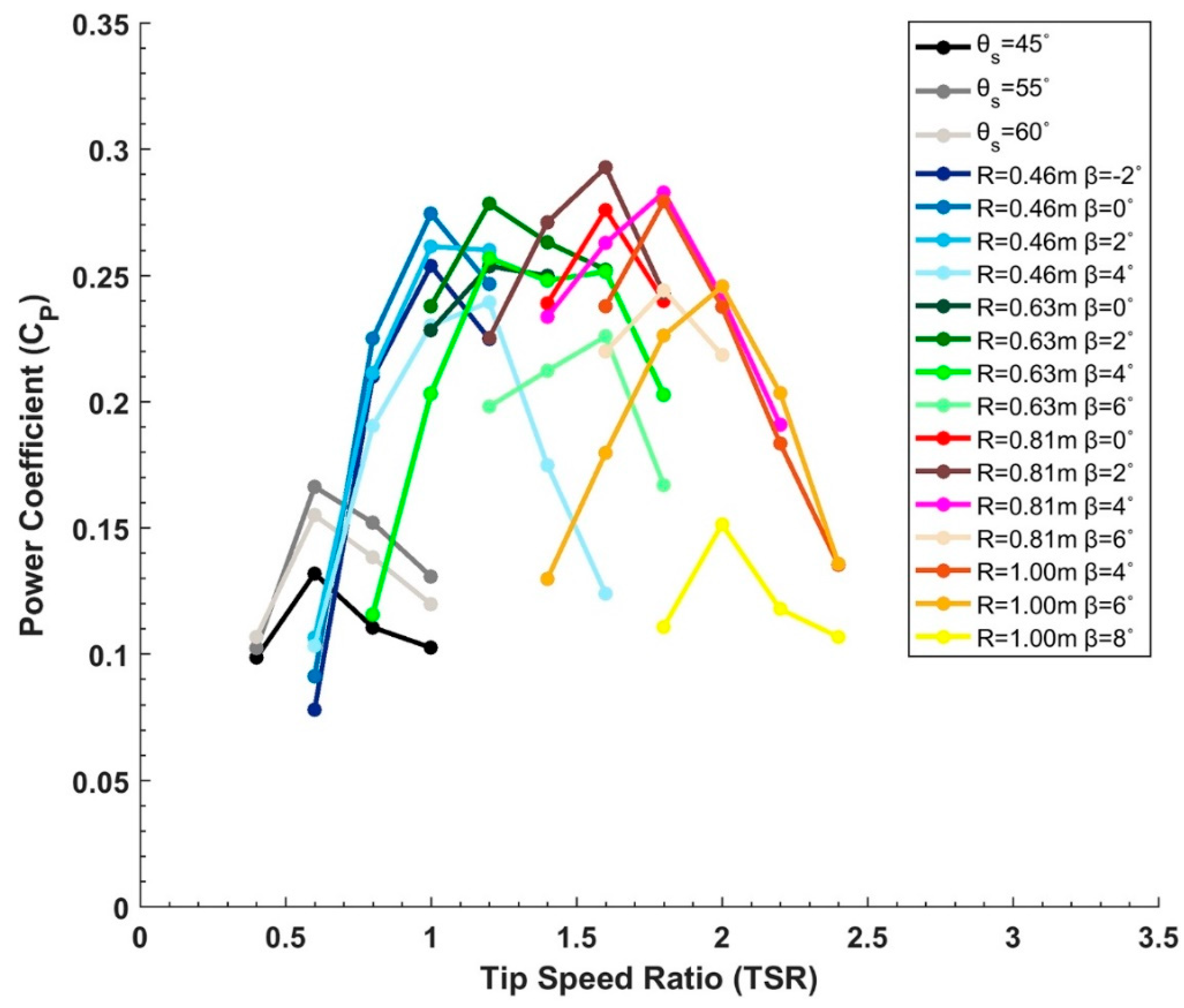
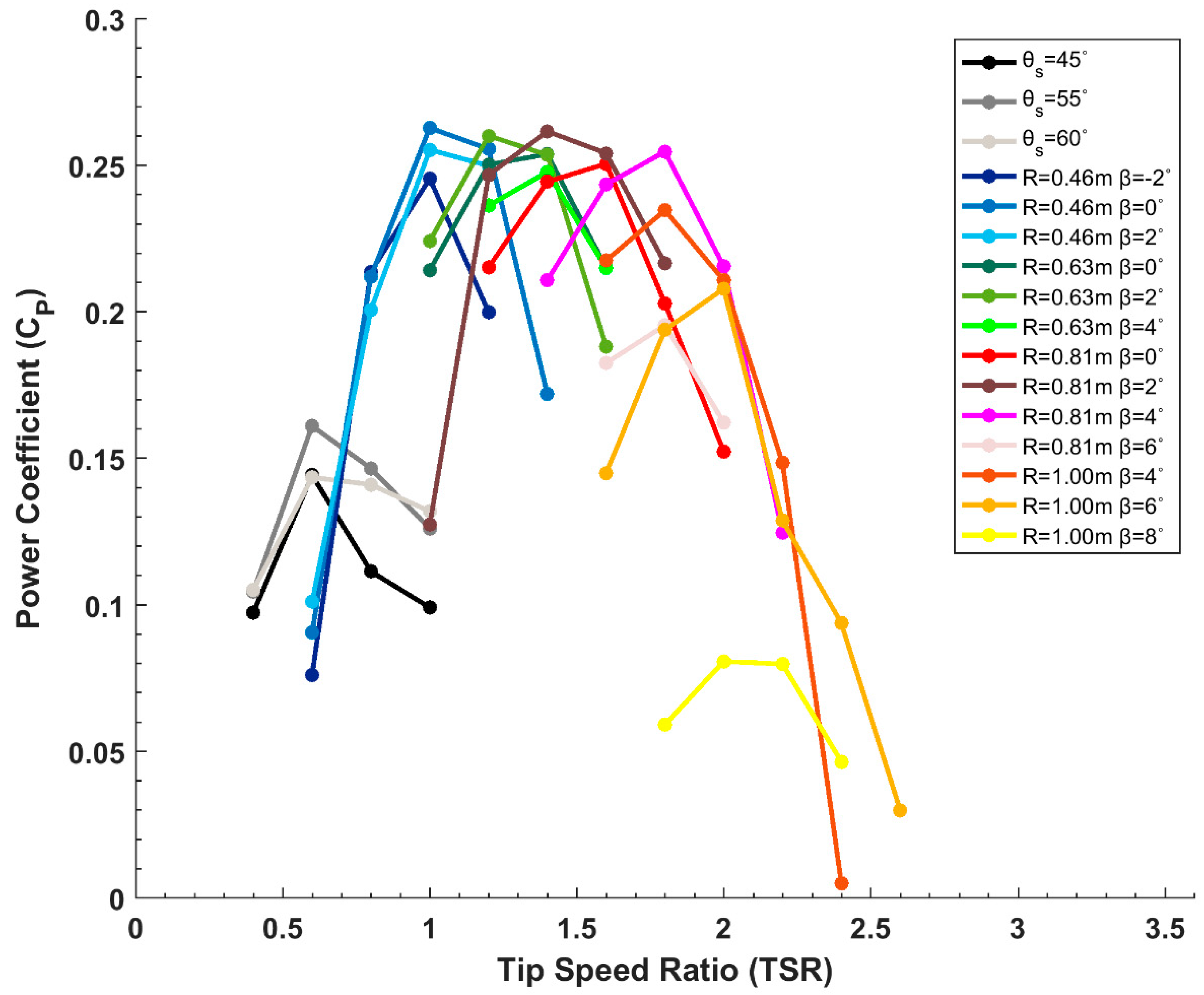
The first step in generating the optimal paths of the blades during the transition process was to find the optimal Savonius configuration. This was accomplished by generating different C
p curves with different values of
, as seen in
Figure 5. It was evident that as the value of
increased from 45° to 55°, the C
p curve shifted upwards attaining a maximum C
p value of 0.166 at TSR = 0.6. However, with a further increase from
= 55° to
= 60°, the C
p curve exhibited a shift downwards. As a result, the optimal value for
was determined to be 55° yielding an optimum R
s of 0.441 m.
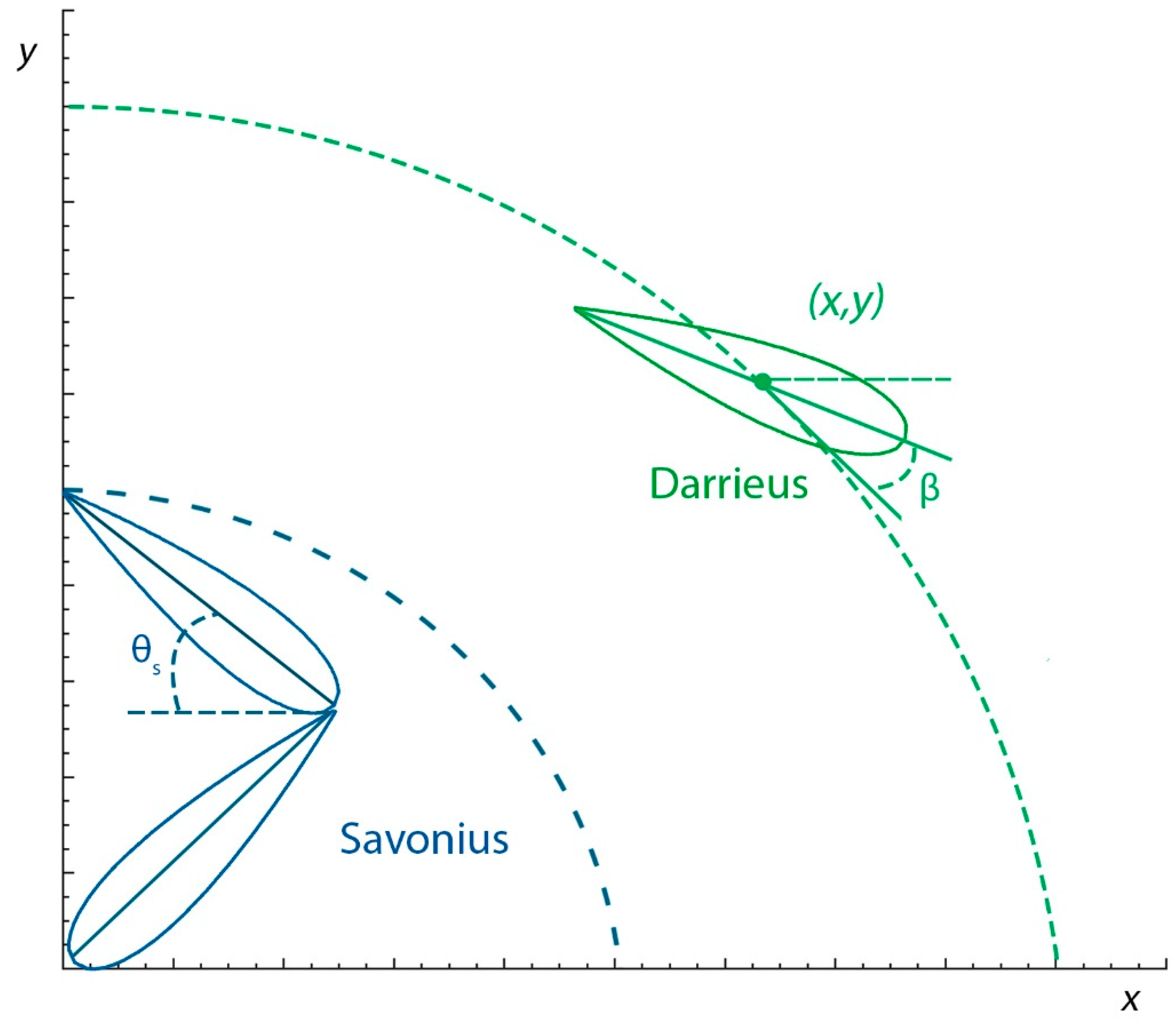
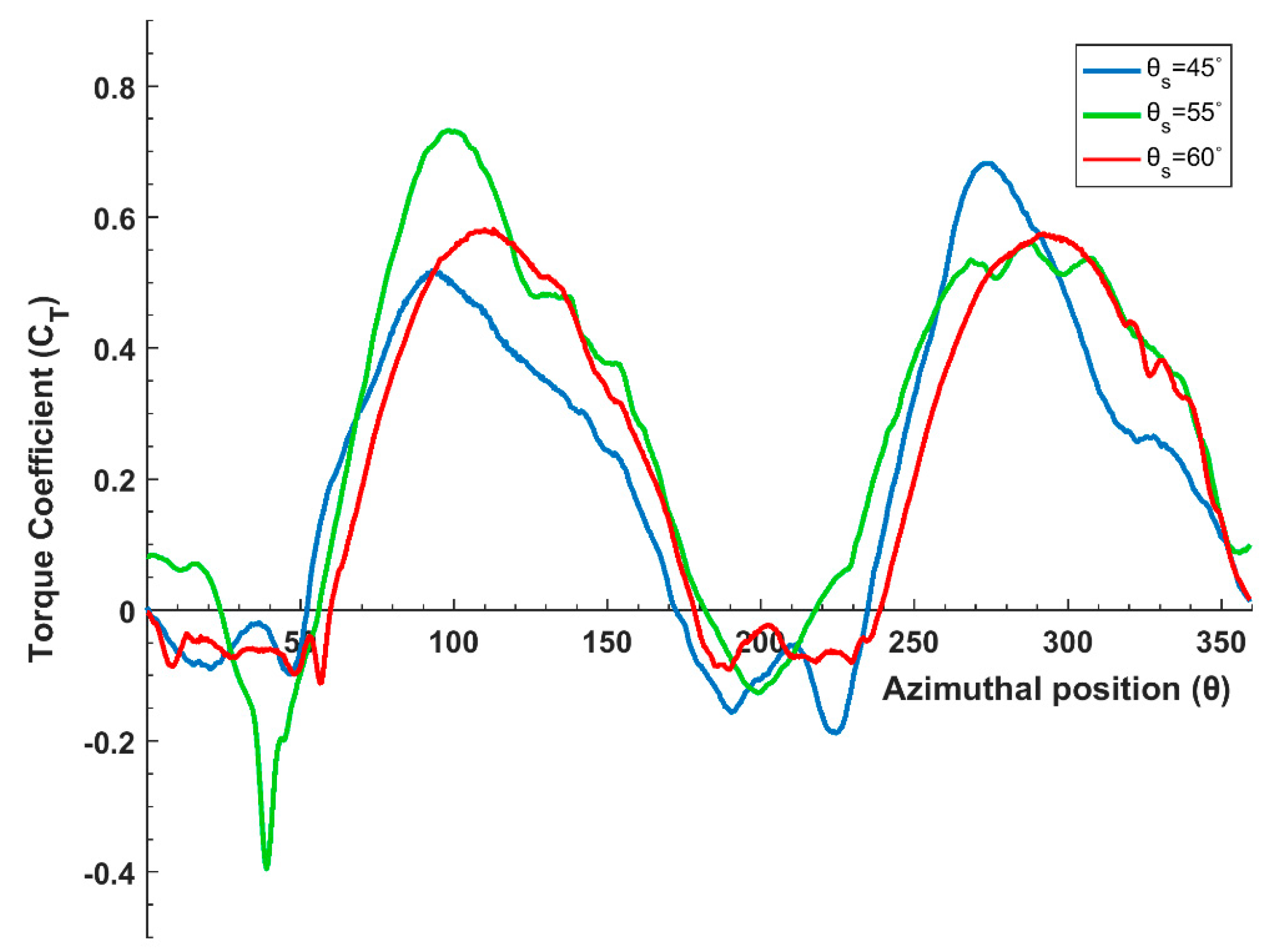
Figure 6 presents the torque coefficient (C
T) variation with azimuthal positions at TSR = 0.6 for the three considered Savonius configurations. Azimuthal position
= 0° was the position where the ends of the Savonius rotor blades coincided with the
y-axis, as shown in
Figure 3, and
increased as the blades rotated clockwise. The averaged C
T values over one rotation were 0.220, 0.278, and 0.259 for
= 45°,
= 55°, and
= 60°, respectively, and it was clear that
= 55° delivered superior performance for most rotors’ azimuthal positions. However, slight exceptions existed at 26°
67° and 260°
288° where the performance of
= 45° was marginally better, as depicted in
Figure 6.
The suggested Savonius configurations adhered to the unique behavior of Savonius turbines by having spells of very high C
T values (
Figure 6). A maximum C
T value of 0.731 was attained by the Savonius turbine with
= 55° at an azimuthal angle
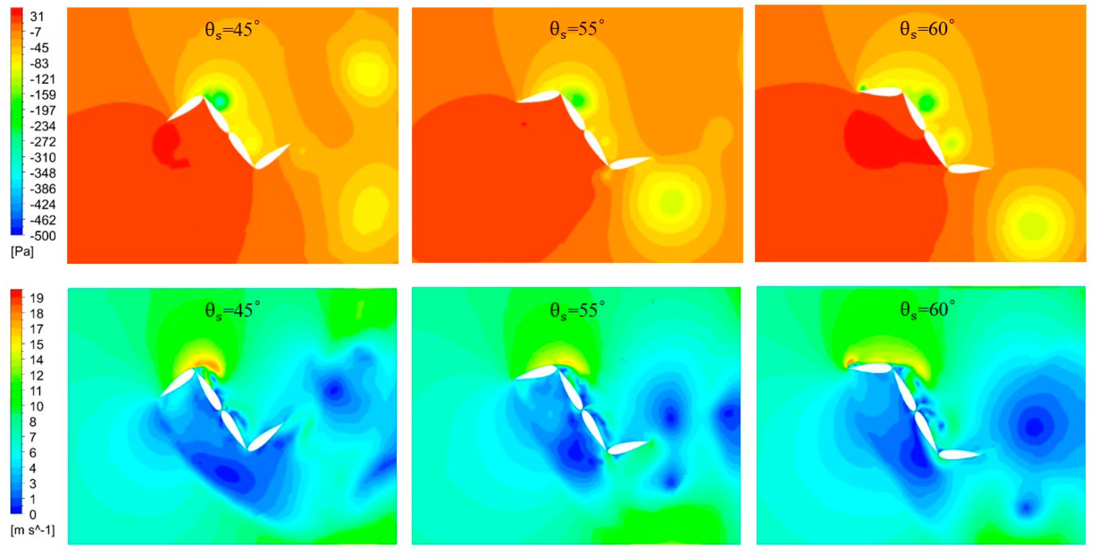
= 100°. The Savonius turbine relied on the difference in pressure between the concave and convex sides of the blades to generate torque. Hence, it was important to visualize the pressure contours at this location in order to obtain further insight. As seen in
Figure 7, the positive pressure area on the returning blade of the Savonius turbine with
= 55° was the smallest compared with the other configurations. Since this positive pressure inhibits the clockwise rotation of the rotor, the configuration with
= 55° developed the least resistance, and consequently generated the largest torque. This can be further explained by analysing the velocity contours (
Figure 7), where it was evident that the stagnation area on the convex side of the returning blade was the lowest for
= 55°, which in turn led to the aforementioned decrease in positive pressure area.
6.2. Darrieus Configurations
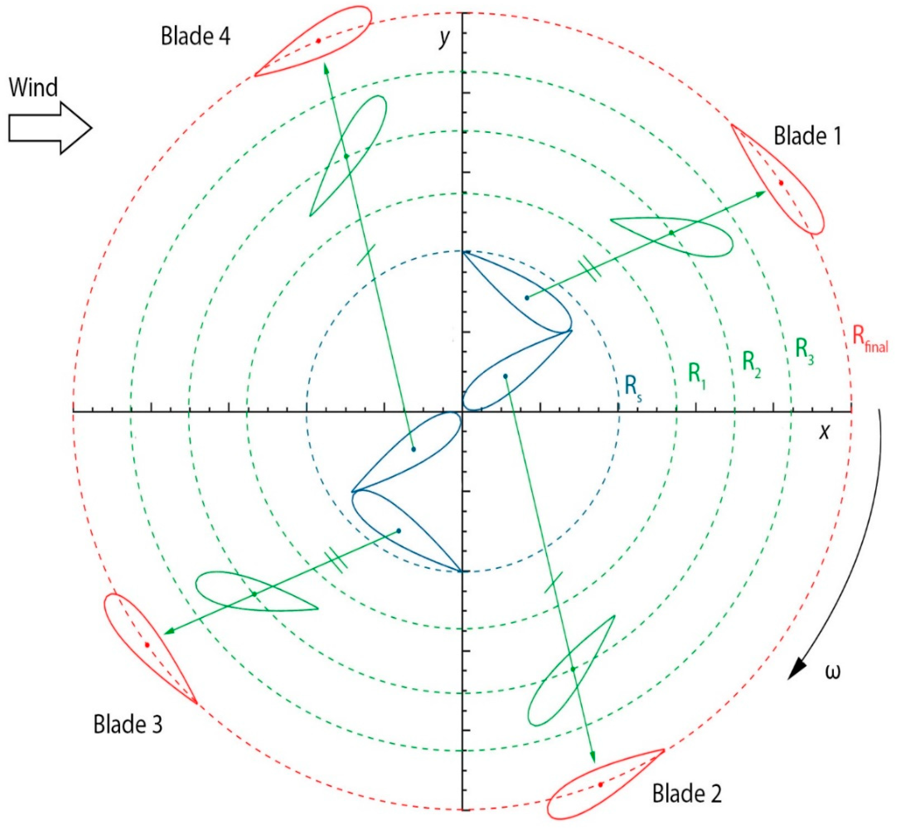
With no variation in its angular orientation, each blade was translated via a unique path from the optimized Savonius configuration of
= 55° in order to attain a desired value of β at R
final. Consequently, β
opt,f was determined by generating different C
p curves with different values of β as seen in
Figure 5. It was evident that the optimum value of the pitch angle (β
opt,f) was 6°, since the turbine’s efficiency was always greater compared to that of β = 4° and β = 8°. It should be noted that the maximum efficiency of this Darrieus turbine was 0.246, which was almost 50% greater than the maximum efficiency of the optimized Savonius configuration. In addition, peak C
p value was attained at TSR = 2.0 for the Darrieus turbine with R = 1 m, where on the other hand, peak C
p was attained at considerably lower TSR = 0.6 for the optimized Savonius turbine. These two unique characteristics are what mainly distinguishes the performances of these two turbines and form the basis for the current study.
With an optimized
= 55° and β
opt,f = 6° at R
final = 1 m, the straight paths of the blades’ centers were generated, as listed in
Table 1. As mentioned earlier, the blades’ transition from R
s = 0.441 m to R
final = 1 m with β
opt,f = 6° was discretized into three optimization stages (R
1, R
2, and R
3) (
Figure 3). The radial increment from one stage to another was selected in a way that would yield similar increments in the
x- and
y-directions for blades 1 and 3. As a result, this yielded R
1 = 0.46 m, R
2 = 0.63 m, and R
3 = 0.81 m.
At the first optimization stage, in order to have R = R
1 = 0.46 m, the blades’ centers had the following coordinates:
x1 = 0.276 m,
y1 = 0.371 m,
x2 = 0.386 m,
y2 = −0.254 m,
x3 = −0.276 m,
y3 = −0.371,
x4 = −0.386 m, and
y4 = 0.254 m. As depicted in
Figure 5, different C
p curves were generated for different values of β. Here again, a vertical shift was evident when the value of β was changed, where it was clear that β = 0° provided the best performance. Compared to the Savonius configuration, the maximum efficiency and the TSR value at which it occurred increased as anticipated. It is evident by now that the Savonius configuration with
= 55° had to be adopted during the start-up phase and up until TSR = 0.6, after which a transitioning process into a Darrieus rotor with R = 0.46 and β = 0° had to take place. Having a small radius, this configuration is characterized by its high solidity
, where
N is the number of blades. During spells of high angle attack (α), complex flow structures evolve around the blades, and shed to impinge on the other blades of this highly packed rotor. The development of these structures and their interactions are responsible for power generation at lower TSRs, where α values are usually very large.
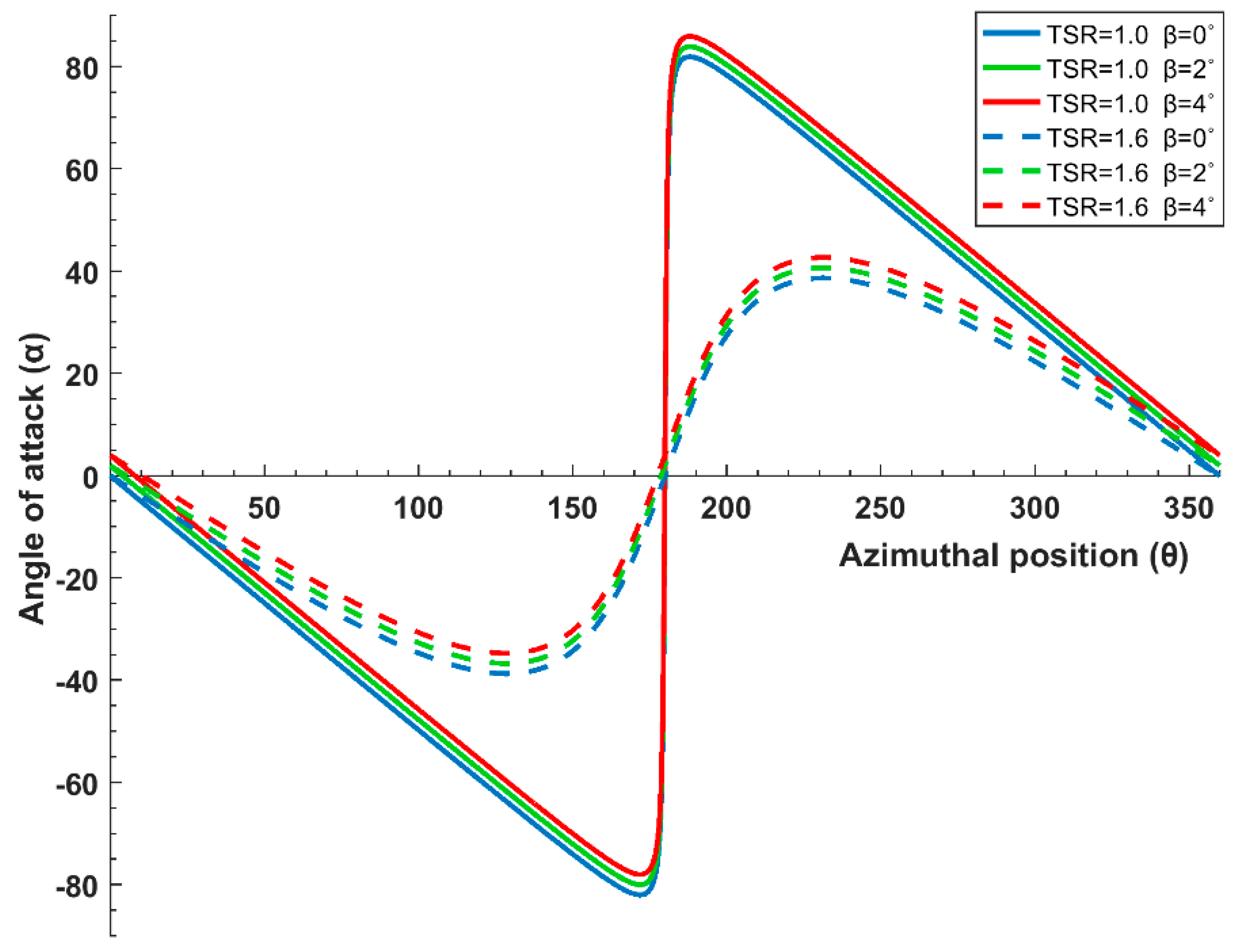
Figure 8 presents the angle of attack variation with
at TSR = 1.0 and TSR = 1.6, with
= 0° being the position where the center of blade 1 coincides with the
y-axis, and increases with the clockwise rotation of the rotor. It is evident that, for all blade pitch angles, the blades experience massively higher angles of attack at TSR = 1.0, compared to the drastically lower α ranges experienced at TSR = 1.6. This is the main reason why C
p peaks at TSR = 1.0, and undergoes a sharp drop at higher TSRs for the turbine with R = 0.46 m (
Figure 5).
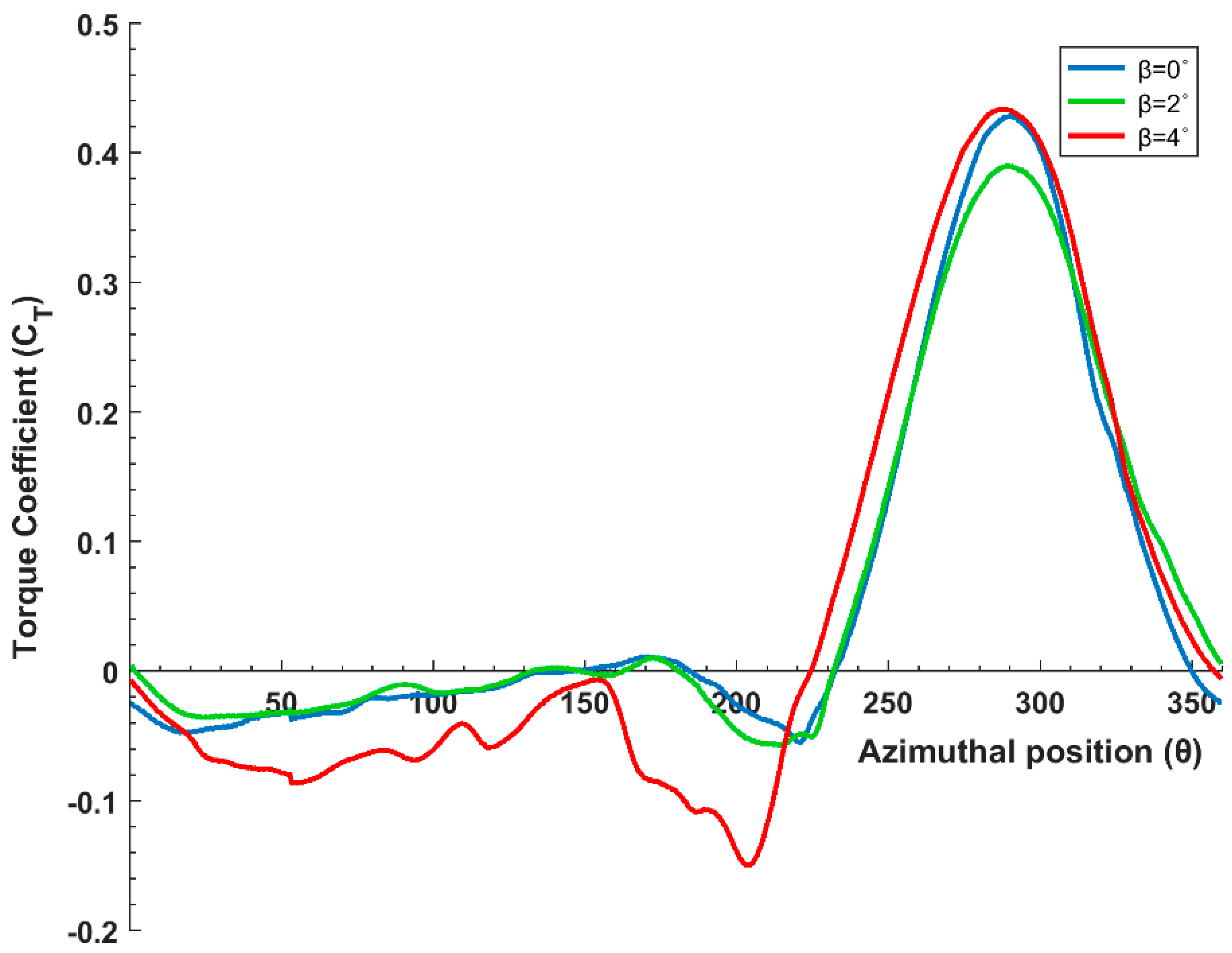
Figure 9 presents the instantaneous torque coefficient variation of a single blade for different β at R = 0.46 m and TSR = 1.0. It is evident that during the downwind cycle (
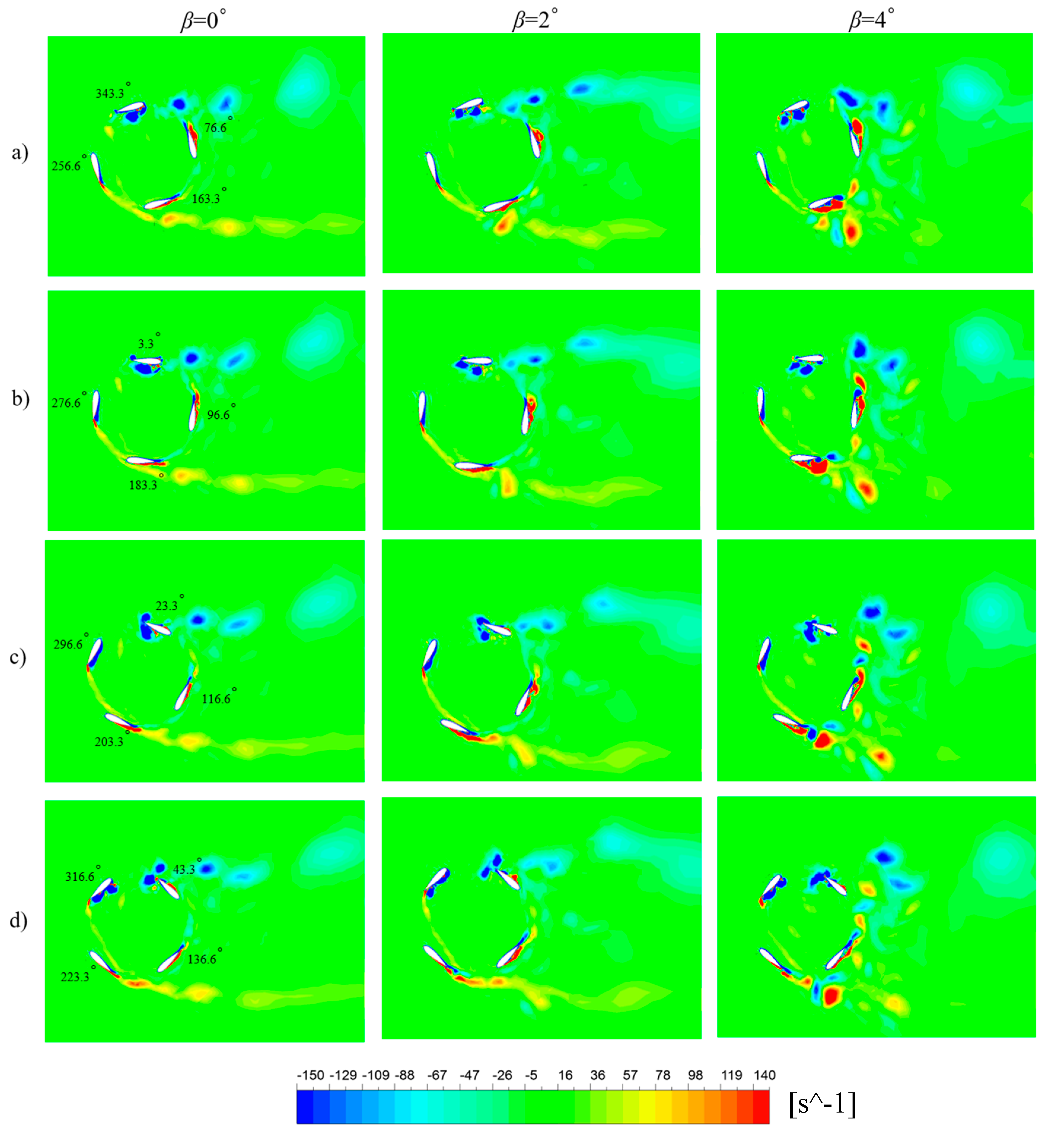
180°), the blade with β = 4° delivers the least amount of torque, while β = 0° and β = 2° have almost the same behavior. In order to further explain this trend, the vorticity field of the configurations with R = 0.46 m and different values of β is shown in
Figure 10. The development and interactions of complex flow structures are evident for this high solidity rotor. At
= 183° (
Figure 10b), a trailing edge vortex at the suction side of blade begins to roll up, and eventually reaches the other side of the blade, where it interacts with the vortex developed during the downwind cycle. With β = 4°, the angle of attack is the greatest at this position and during the rest of the upwind cycle. This is why the aforementioned vortex behavior is most prominent for this value of β. As seen in
Figure 10c, this results in the periodic shedding of strong counter rotating vortices towards the top-right corner, which then impinges into the suction side of the following blade during its downwind journey. As a result of these interactions, the strength of the vortex core developed on the following blade increases, and this is the main reason why the turbine with β = 4° generates the least amount of torque for
180°. Moving to the upwind cycle (
≥ 180°), it is clear that the blade with the highest pitch angle delivers the greatest amount of torque (
Figure 9). This can also be attributed to the fact that the angle of attack is the greatest for β = 4° during this cycle, which leads to the development of stronger vortices on the suction side of the blade
Figure 10c (
= 296.6°). Consequently, this lowers the pressure on the suction side of the blade to a greater extent, and therefore leads to the generation of more torque during the upwind cycle.
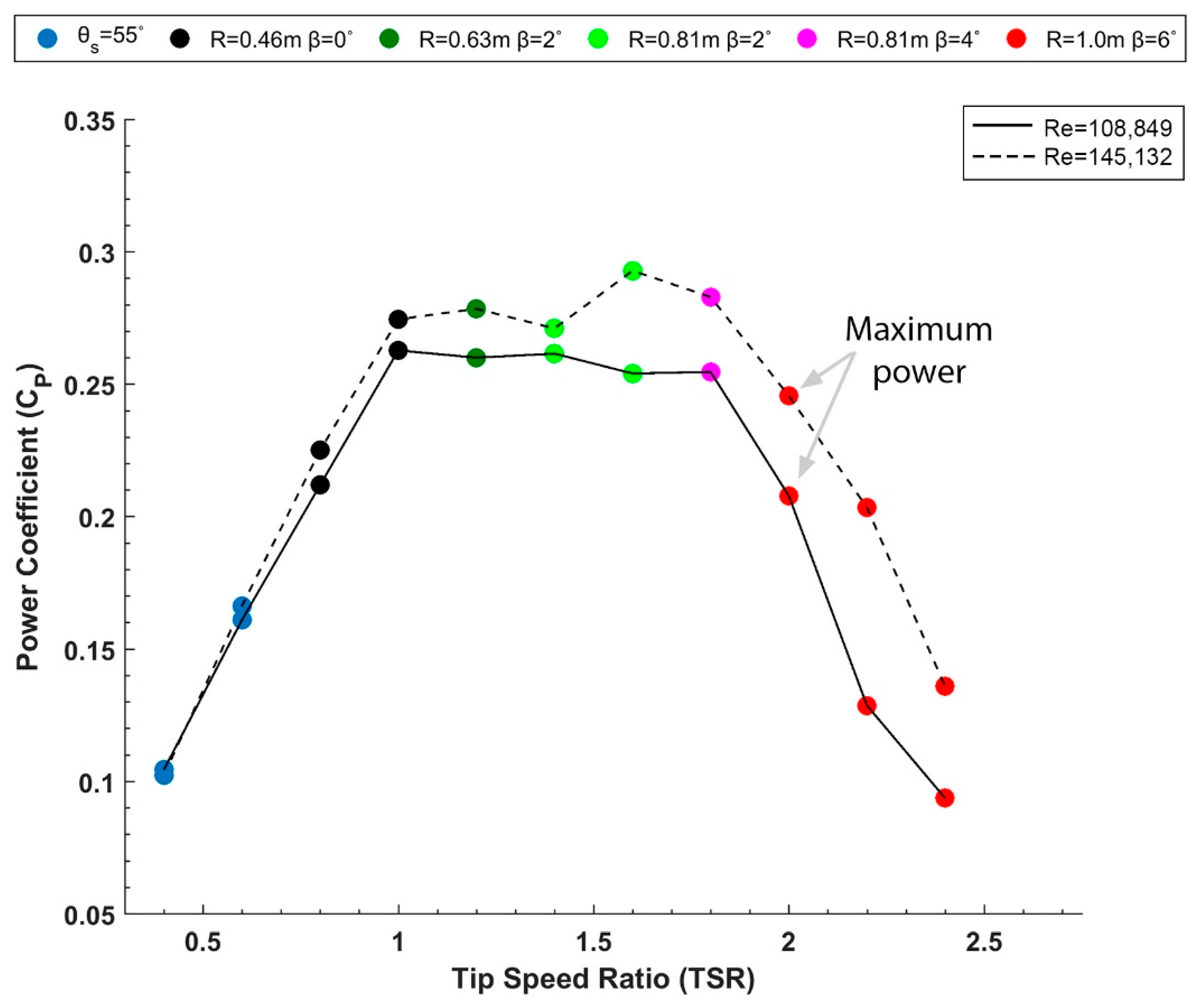
Moving on to the second optimization stage at R = R2 = 0.63 m, the coordinates of the blades’ centers were set as follows: x1 = 0.475 m, y1 = 0.409 m, x2 = 0.494 m, y2 = −0.385 m, x3 = −0.475 m, y3 = −0.409, x4 = −0.494 m, and y4 = 0.385 m. The blade pitch angles were varied and different Cp curves were generated. As expected, the location where the Cp curve peaks shifts to the right with increasing rotor radius. The maximum Cp developed was equal to 0.279 at TSR = 1.2 for the configuration with β = 2°, which provides superior performance compared with other pitch angles. Hence, at this stage, it is clear that the turbine has to transition to R = 0.63 and β = 2° at TSR ≥ 1.2.
At the final optimization stage, with R = R
3 = 0.81 m, the coordinates of the blades’ centers were:
x1 = 0.675 m,
y1 = 0.447 m,
x2 = 0.613 m,
y2 = −0.529 m,
x3 = −0.675 m,
y3 = −0.447 m,
x4 = −0.613 m, and
y4 = 0.529 m. As evident from
Figure 5, the peak location of the C
p curve again shifts to the right with an increase in the rotor’s radius. Regarding the sampled values of β, it was clear that a vertical shift in the C
p curve takes place when β increases from 0° to 2°, where a maximum C
p value of 0.293 is attained at TSR = 1.6. However, when β is further increased to 4°, a horizontal shift in the C
p curve takes place, where peak C
p = 0.283 is attained at TSR = 1.8. Finally, with an increase in β to 6°, the C
p curve moves vertically downwards, where the turbine’s performance is deteriorated. Therefore, due to this noticeable horizontal shift in the C
p curve with changing β, it can be concluded that for maximum efficiency, the turbine has to shift to R = 0.81 m with β = 2° for TSR
1.4, and to β = 4° for TSR > 1.6.
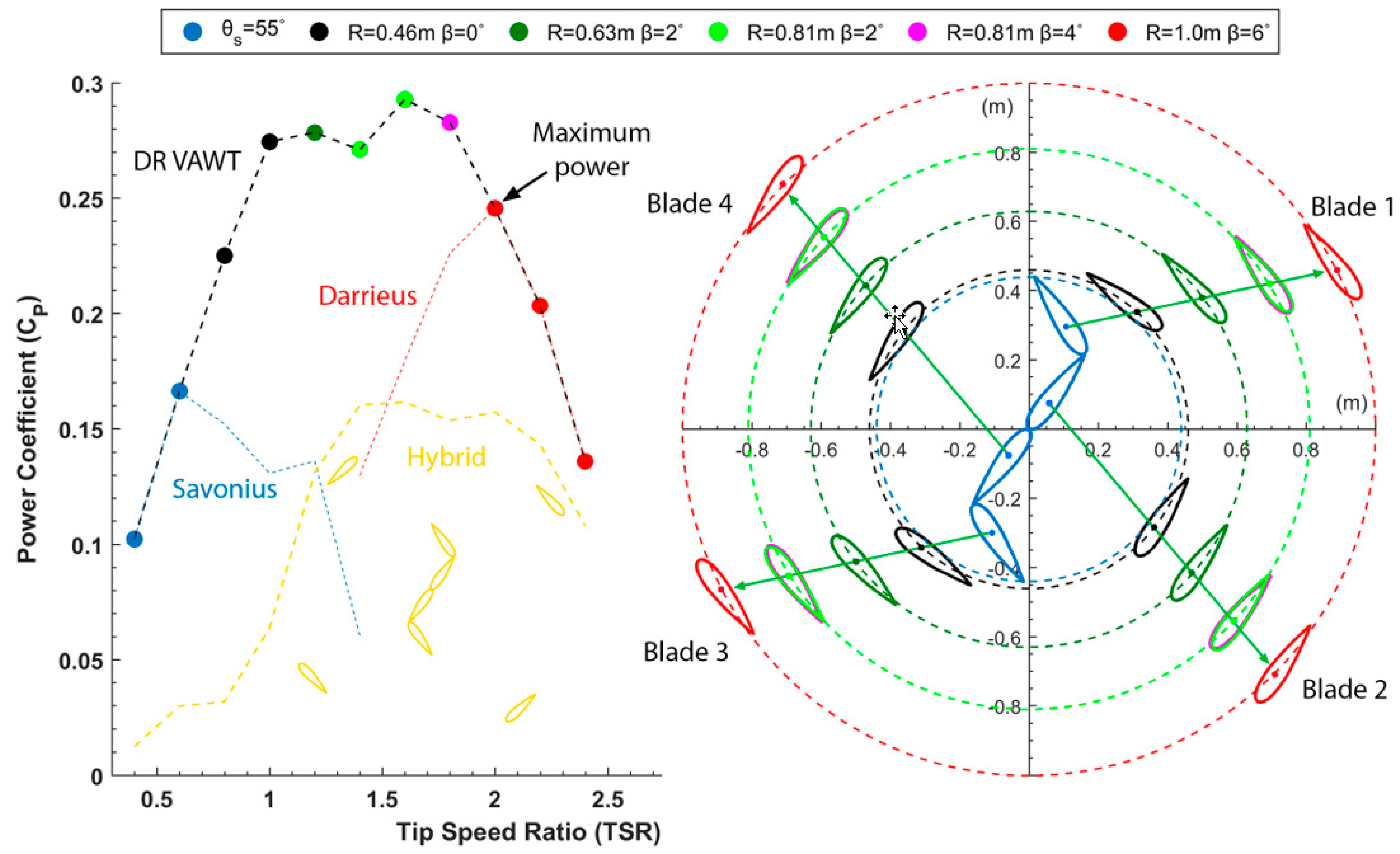
6.3. Optimized DR VAWT
After generating all the necessary C
p curves, it is evident that the optimized dynamic turbine has to transition into its final position of R = R
final = 1 m with β = 6° at TSR
2.0.
Figure 11 provides a clear illustration of the overall performance of the optimized DR VAWT and its blades trajectories. It is evident that the range of operational TSR where the turbine attains decent performance has drastically increased. The average power coefficient (C
p,avg) is defined as:
where n = 11 is the total number of sampled C
p,i values at different TSRs {0.4, 0.6, 0.8, … 2.4}. C
p,avg for the optimized DR VAWT was equal to 0.225, which was 192% higher when compared to the Savonius configuration with C
p,avg = 0.077, and 87.5% higher when compared to the Darrieus configuration at R
final with C
p,avg = 0.120. Thus, it can be confidently said that the goal of maximizing the operational TSR range and the average power coefficient while maintaining a low cut-in speed was successfully accomplished.
Figure 11 also presents the power coefficient curve for a turbine with a hybrid Savonius–Darrieus rotor with
= 55°, R = 1 m, and β = 6°. The resulting C
p,avg of the hybrid turbine was equal to 0.102, and was considerably (55%) lower than the average C
p produced by the optimized DR VAWT.
The power (P) generated by the turbine is given by:
where H is the extrusion height of the turbines’ blades. Since only R and
terms vary across the different configurations during the transitioning process, the point with maximum
will generate maximum amount power for the DR VAWT configuration at a given wind speed. At TSR = 2.0, R = 1 m, and β = 6° (
Figure 11), the maximum value of
= 0.246 m was attained. Therefore, if the load on the turbine, hence, the rotational velocity can be controlled, one can seek to operate at the point of maximum power (R = 1), while extensively benefiting from the excellent start-up characteristics of the Savonius configuration, and the efficient transitioning process into the final Darrieus position.
6.4. Effect of Reynolds Number
In order to validate the generated optimal blade trajectories, and analyze their sensitivity to wind velocity, a similar optimization process was repeated for a free-stream wind velocity of 6 m/s. This yielded a chord-based Reynolds number of 108,849.
Figure 12 shows the power coefficient values at different TSRs for all the sampled configurations at Re = 108,849, where it was evident that the optimal Savonius configuration
= 55° remained the same. Moving on to the final radius (R
final = 1 m), β = 6° provided superior performance compared with other β values. Hence, the straight paths of the blades’ centers were generated and were identical to the ones generated for Re = 145,132. This was because both yielded similar optimized initial and final positions. Consequently, the optimization stages (R
i) were also identical to the ones chosen in
Section 5.2, with radii R
1 = 0.46 m, R
2 = 0.63 m, and R
3 = 0.81 m.
As evident from
Figure 12, different values of β were analyzed at the three optimization stages, and a shift in the peak location was observed when increasing the rotor radius. At R = R
1 = 0.46 m, the turbine with β = 0° provided the greatest efficiency, where it was clear that a transitioning process should occur from
θs = 55° to this configuration at 0.6 < TSR < 1.2. At R = R
2 = 0.63 m, β = 2° performed best, and therefore, this configuration should be adopted at 1.2 ≤ TSR ≤ 1.4. Moving on to the final optimization stage with R = R
3 = 0.81 m, a similar phenomenon was replicated from the analysis with Re = 145,132, where two optimum values for β co-existed at different TSR ranges. For optimal performance, the turbine should have R = 0.81 m and β = 2° at 1.4 ≤ TSR ≤ 1.6, and R = 0.81 m and β = 4° at 1.6 < TSR < 2. A final transitioning process into R = R
final = 1 m and β = 6° should occur at TSR ≥ 2.0. If compared with the generated results from the previous analysis with Re = 145,132, the aforementioned optimal blades’ positions were exactly identical at their respective TSRs. Moreover, the point of maximum power generation (TSR = 2.0, R = 1 m, and β = 6°) was similar in both cases as well. This establishes a solid basis for rendering the optimized blades’ trajectories independent of Re values.
The efficiency of the optimized DR VAWT decreased with decreasing Reynolds number as evident in
Figure 13. At the lower Reynolds number, a maximum C
p of 0.263 and an average C
p of 0.200 were obtained, and both were lower than the maximum C
p = 0.293 and C
p,avg = 0.225 of the higher Reynolds number case. The difference in C
p values was minimal at lower TSRs; however, it started to increase at higher TSRs, where the biggest difference was observed at TSR = 1.6 (
Figure 13). Hence, it can be deduced that the effect of varying the Reynolds number simply resulted in a vertical shift in the overall power coefficient curve. This is typical behavior of VAWTs, which is commonly referred to in the literature [
32,
33].
6.5. Effect of Blades’ Trajectories
Another sensitivity analysis was conducted on the blades’ optimized trajectories. The performance of the DR VAWT, with the following trajectories was compared to the optimized ones:
Zigzag trajectories: Each blade center followed a zigzag path, composed of four straight lines so that the optimal value of β was achieved at the corresponding radius and TSR. Each blade was allowed to translate while having fixed, angular orientations (
Figure 14, green).
Straight trajectories: Each blade center followed the optimal straight path at the respective TSR (
Table 1), with its angular orientation kept fixed. This means that there was no control over the pitch angle (β) when varying the radius, as seen in
Figure 14 (red).
The fixed, angular orientations of the blades were based on the optimized Savonius configuration (
= 55°) as discussed earlier.
Figure 14 shows the power coefficient distribution for the DR VAWT following the zigzag and straight blades’ trajectories, with the optimized ones shown in blue. Since in all the simulated cases, the blades started from the same Savonius position, the performance of the optimized DR VAWT was replicated by both cases at TSR ≤ 0.6. Moving on to radius R
1 = 0.46 m, it was evident that the zigzag trajectories yielded C
p values that were closer to the optimized configuration than the straight trajectory, with a maximum performance drop equal to 9% at TSR = 1.0. It can be seen from
Figure 14 that the blades’ positions for the zigzag trajectories differred compared to the optimized ones at R = R
1 = 0.46 m. Since blade vortex interactions are prominent for this high-solidity rotor, as previously discussed, changing the relative distances between the rotor’s blades was anticipated to have a slight influence on performance, even though both the zigzag and optimized cases have the same values of β at the respective R and TSR. When it comes to the straight trajectories at R
1, the performance was heavily deteriorated, and the power generated by the turbine was minimal. The main reason behind this performance drop was the inability to control the blade’s angular orientation while transitioning along a straight path. Consequently, random values of the pitch angle β were obtained along the straight path causing a negative influence on the turbine’s performance.
Table 2 provides a comparison between the resulting values of β for all the blades when transitioned along a straight path without changing the angular orientations (straight trajectories). Note that blades 1 and 3 will have the same β values due to their identical blade center paths as discussed previously (same applies to blades 2 and 4). It was evident that at R = R
1 = 0.46 m, β = −18.36° for blade 1, which massively differed from the optimal value of 0°. This was the main reason why the DR VAWT following the straight trajectories generated minimal amounts torque-generating lift forces at R
1.
At R = R
2 = 0.63 m, the blades’ positions following the zigzag trajectories still differ compared to the optimized configuration, and thus, C
p slightly dropped by 5%. Regarding the case with straight trajectories, the resulting pitch angle at R
2 is still negative (−5.69°) and differs from the optimal value of 2°, however to a lower extent this time. As a result, the DR VAWT with straight blades trajectories yields a value of C
p = 0.21 at TSR = 1.2. Moving on to R = R
3 = 0.81 m, the performance of the optimized turbine was replicated by the zigzag trajectories since the blades’ positions were identical to a large extent, as seen in
Figure 14. The case with the straight trajectories also yielded a decent performance, however, with slightly lower C
p values compared to the optimized DR VAWT. At R
3, the optimal value for β was equal to 2° at 1.4 ≤ TSR ≤ 1.6, and equal to 4° at 1.6 < TSR ≤ 1.8. Since β = 1.5° for blade 1, which slightly differed from the optimal value, this constituted the main cause of the aforementioned performance drop. Overall, it can be said that adopting a mechanism that allows each blade center to follow a zigzag path without changing its angular orientation will provide an overall turbine performance close to the optimized one, since C
p,avg = 0.219, which is only 2.7% lower compared to C
p,avg = 0.225 of the optimized configuration. However, utilizing a simple mechanism that simply translates each blade center along a straight path without altering its angular orientation will yield poor efficiency at 0.6 < TSR ≤ 1.0 with an overall C
p,avg = 0.169, corresponding to a drop by 24.8%.
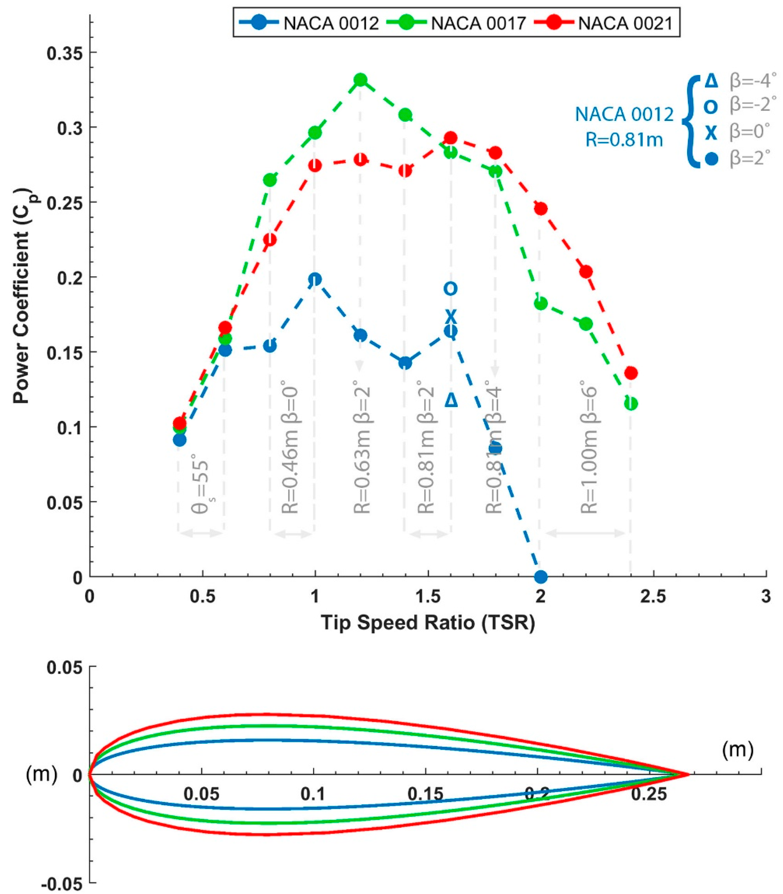
6.6. Effect of Airfoil Thickness
For a conventional four-digit NACA airfoil, the third and fourth digits represent the maximum airfoil thickness as a fraction of the chord length. The maximum thickness is located at 0.3 c from the leading edge of the airfoil. In the current work, optimal blades’ trajectories were generated while adopting NACA 0021 airfoil sections, as mentioned earlier. To study the influence of the airfoil thickness, the performance of the DR VAWT with the optimized blades’ trajectories was assessed utilizing two other airfoil sections: (1) NACA 0012 and (2) NACA 0017. The resulting power coefficient values are presented in
Figure 15. It was evident that all cases generated the same amount of power at the Savonius configuration (TSR ≤ 0.6). This was anticipated since the Savonius turbine is a drag-based turbine, relying primarily on the drag forces resulting from the separated flow pressure differences between both sides of the turbine’s blades. Since altering the airfoil thickness does not have a considerable influence on the flow mechanisms, and ultimately on the generated pressure difference for a Savonius configuration, the performances of all three airfoil thicknesses were identical. However, the airfoil’s thickness had a considerable influence on the stalling characteristics, and pressure distributions of a Darrieus type VAWT according to several studies [
34,
35,
36]. As seen in
Figure 15, the power coefficient of the NACA 0017 and NACA 0021 configurations increased to an optimal value, and then decreased with increasing TSR for the Darrieus configurations. Additionally, the location where maximum C
p value occurred was different for both cases. Maximum C
p = 0.332 for the NACA 0017 configuration occurred at TSR = 1.2, while maximum C
p = 0.293 for the NACA 0021 configuration occurred at TSR = 1.6. The average power coefficient equalled 0.255 for both cases; however, the former performed better at lower TSRs (TSR < 1.6) and higher turbine solidity, while the latter delivered superior performance at higher TSRs (TSR ≥ 1.6) and lower solidities. Increasing the airfoil’s thickness by 4% (from NACA 0017 to NACA 0021) increased the radius of curvature at the airfoil’s leading edge. This, in turn, leads to smoother pressure differentials, and is the primary reason why thicker airfoils provide better stalling characteristics for the DR VAWT especially at higher TSRs. This also explains the heavily deteriorated performance resulting when adopting thinner NACA 0012 airfoil sections, where C
p,avg = 0.128 and the operational TSR range is narrowed (
Figure 15). It is worth noting that the utilized pitch angles for all airfoil sections were extracted while utilizing NACA 0021 airfoils. Consequently, one may attribute the drop in performance to the fact that the DR VAWT with NACA 0012 airfoils was not operating at its optimal conditions. However, as seen from
Figure 15, even when the performance of the former was optimized by having β = −2° at R = 0.81 m and TSR = 1.6, for instance, the optimized C
p value was still drastically lower compared to that of the optimized thicker airfoil sections. Hence, thin airfoil sections are clearly not suitable for the proposed DR VAWT.


