Two-Stage Energy Management Strategy of EV and PV Integrated Smart Home to Minimize Electricity Cost and Flatten Power Load Profile

Abstract

The efficient use of the incorporation of photovoltaic generation (PV) and an electric vehicle (EV) with the home energy management system (HEMS) can play a significant role in improving grid stability in the residential area and bringing economic benefit to the homeowner. Therefore, this paper presents an energy management strategy in a smart home that integrates an electric vehicle with/without PV generation. The proposed strategy seeks to reduce the household electricity costs and flatten the load curve based on time-of-use pricing, time-varying household power demand, PV generation profile, and EV parameters (arrival and departure times, minimum and maximum limit of the state-of-charge, and initial state-of-charge). The proposed control strategy is divided into two stages: Stage A, which operates in three operating modes according to the unavailability of PV power generation, and Stage B, which operates in five operating modes according to the availability of PV generation. In this study, the proposed strategy enables controlling the amount of energy absorbed by the EV from the grid and/or PV and the amount of energy injected from the EV to the load to ensure that the household electricity costs are minimized, and the household power load profile is flattened. The findings show that both household electricity costs reduction and flattening of the power load profile are achieved. Moreover, the corresponding simulation results exhibit that the proposed strategy for the smart home with EV and PV provides better results than the smart home with EV and without PV in terms of electricity costs reduction and power load profile flattening.

1. Introduction

Fossil fuel shortage and the increase of environmental pollution caused by the transport and power sectors have become serious global issues [1,2]. Therefore, the need for a more effective way to reduce fuel dependency and environmental pollution reduction has led to the emerging of renewable energy technologies and electric vehicles (EVs) in the power and transport sectors, respectively [3,4,5]. However, production instability of variable renewables such as wind power and solar photovoltaics and intermittent charging patterns of EVs can lead to several problems in the power grid such as growing demand peaks, voltage fluctuations, high load variability, and over-generation [6,7]. These challenges require effective energy management to adapt between electric vehicles charging patterns and renewable energy generation [8,9]. As a result, recent studies have focused on developing effective energy management to integrate renewable energy and EVs into homes and grid. With the advent of the smart grid concept and thanks to bi-directional communication technologies provided by the smart meters between utilities and smart homes, smart homes have gained many advantages and opportunities, such as economic incentives and improved energy consumption. In addition, under an environment of the smart grid and advancements in home area networks (HAN), homeowners can control their consumption, storage, and generation through the home energy management systems (HEMS) [10,11,12]. Home energy management systems (HEMSs) automatically schedule the household appliances, electric vehicles, and distributed residential energy resources based on time-varying price aiming to reduce the household electricity cost and the stress on the grid utility while satisfying their energy requirements [12,13,14].

Lately, the topic of HEMS integrated with electric vehicle (EV) has attracted the attention of many researchers. Some studies are focusing on cost reduction [15,16]. In [15], the study examined the charging/discharging strategy of electric vehicle (EV) in HEMS to assess the economic benefit of various operation modes such as vehicle-to-grid (V2G), vehicle-to-home (V2H), and grid-to-vehicle (G2V) in dynamic pricing schemes. The stochastic dynamic programming of optimal energy management in the smart home equipped with an electric vehicle was proposed in [16], aiming to reduce electricity costs while satisfying the requirements of electric vehicle charging and household energy demand. The time-varying home power demand and the time-varying electricity price have been used to define different operation modes such as grid-to-vehicle (G2V), vehicle-to-grid (V2G), and vehicle-to-home (V2H). In contrast, the electric vehicle battery equivalent circuit and probabilistic of the length and time of the trip were used to formulate the stochastic optimization problem for an electric vehicle to manage the energy in the smart home. In the same context, other works focused on flattening the variation of the load power profile [17,18]. In [17], the study presented a flexible control strategy for a smart home equipped with two electric vehicles to reduce load variation and flatten the load curve. The flexible control strategy monitors the system in different operation modes according to a set of constraints: (i) the daily power load curve of the household appliances; (ii) electric vehicles connection time; (iii) the state of charge (SOC) of each vehicle battery; and (iv) priority order of each vehicle. In this algorithm, it is noticeable that the time-varying electricity price was not used within system monitoring constraints. Moreover, a double-layer energy management strategy for a smart home equipped with appliances and electric vehicles was proposed in [18] to smooth the load demand profile in a residential application. The authors divided the home energy management into two layers: The first layer focused on-demand response to shifting the appliances from peak to off-peak hours. Simultaneously, the second layer focused on controlling bidirectional power flow among electric vehicles and the smart grid to schedule electric vehicles charging and discharging. It should be noted that, in the first layer, the power load curve and time-varying electricity price were used to shift the appliances from the peak to off-peak hours, while, in the second layer, the power load curve was used, but the time-varying price was not used in scheduling the charging and discharging of an electric vehicle, which will lead to an increase in electricity costs at home. Other studies focused on two folds in reducing household cost and grid stress. For example, the authors of [19] presented heuristic method for detecting the most suitable time to charge/discharge the EV battery at home during the day time regime, depending to household demand, real-time price signal, and EV parameters, in order to minimize household electricity bill and grid stress.

Moreover, several studies have addressed HEMS integration with PV and EV [20,21,22,23]. In [20], HEMS based on mixed-integer linear programming (MILP) model was suggested for smart home consist of small-scale distributed photovoltaic, EV, and energy storage system (ESS) in order to decrease the total consumption of daily electricity cost. In [21], the scholars proposed a new energy management control based on stochastic optimization for the smart home with PV array and EV as energy storage to reduce consumer energy charges while satisfying the household power demand and the EV battery charging requirements. The study in [22] proposed coordinated energy management based on an energy price tag (EPT) for a smart house equipped with PV, EV, and home battery storage to minimize the overall energy cost while meeting storage devices charging requirements and household power demand. Besides, energy management based on a hierarchical deep reinforcement learning approach was designed for a smart home equipped with a rooftop photovoltaic system, electrical appliances, ESS, and EV to reduce electricity costs [23].

Considering the valuable contributions introduced by the studies mentioned above, however, it is notable that the integration of the home energy management system (HEMS) with PV and EV focused on reducing the energy cost ignored the importance of flattening the load curve. The studies that focused on reducing energy cost and flattening the load curve has not included PV generation as part of its system. Besides, some literature focused on flattening the load curve by charging the electric vehicle to fill the valley and discharging to shave the peak load based on the daily household load curve only and ignoring the change of electrical price with time, and this will lead to an increase in the electric energy costs at the home. Therefore, it is interesting to develop a novel energy management strategy for a smart home equipped with an electric vehicle EV and PV. The main objective is to control the amounts of energy flow to/from electric vehicle flexibly to minimize the electricity cost and flatten the load curve with satisfying the system power requirements. As the main contribution of this study, the system is monitored through two stages, each stage activated by several modes according to the following restrictions: daily PV power generation profile, real-time price signal, daily power load curve for household appliances, arrival and departure time of electric vehicle, and minimum and maximum limit state-of-charge of the electric vehicle battery.

The proposed strategy is applicable for any home equipped with PV and EV which can bring economic benefits to the homeowner and can provide support for the residential area grid by charging the EV from the grid and PV generation when the electricity price and consumption are low and PV generation greater than the load to be covered by PV generation respectively. Besides, the energy stored from the grid and PV in EV battery can be used later at peak time.

This paper discusses the home energy management system (HEMS); it is the most important issue that helps to reduce electricity costs, enhance the energy efficiency, and flatten the load curve. The main advantage of the proposed strategy lies in the flexibility of the power flow from grid-to-vehicle (G2V), PV-to-vehicle (PV2V), and vehicle-to-home (V2H). Indeed, the control of EV charge/discharge and EV utilization as energy storage provides the possibility of transmitting valley electricity and PV generation to the peak hours through the vehicle-to-home (V2H), which is one of the modern technologies that help decrease electricity cost and flatten the load curve.

The remaining of the paper is arranged as follows: Section 2 presents the studied system description and modeling. The proposed home energy management strategy is illustrated in Section 3, and the economic analysis is detailed in Section 4. Simulation results are discussed in Section 5. Finally, Section 6 elaborates the conclusion of this paper.

2. System Description and Modeling

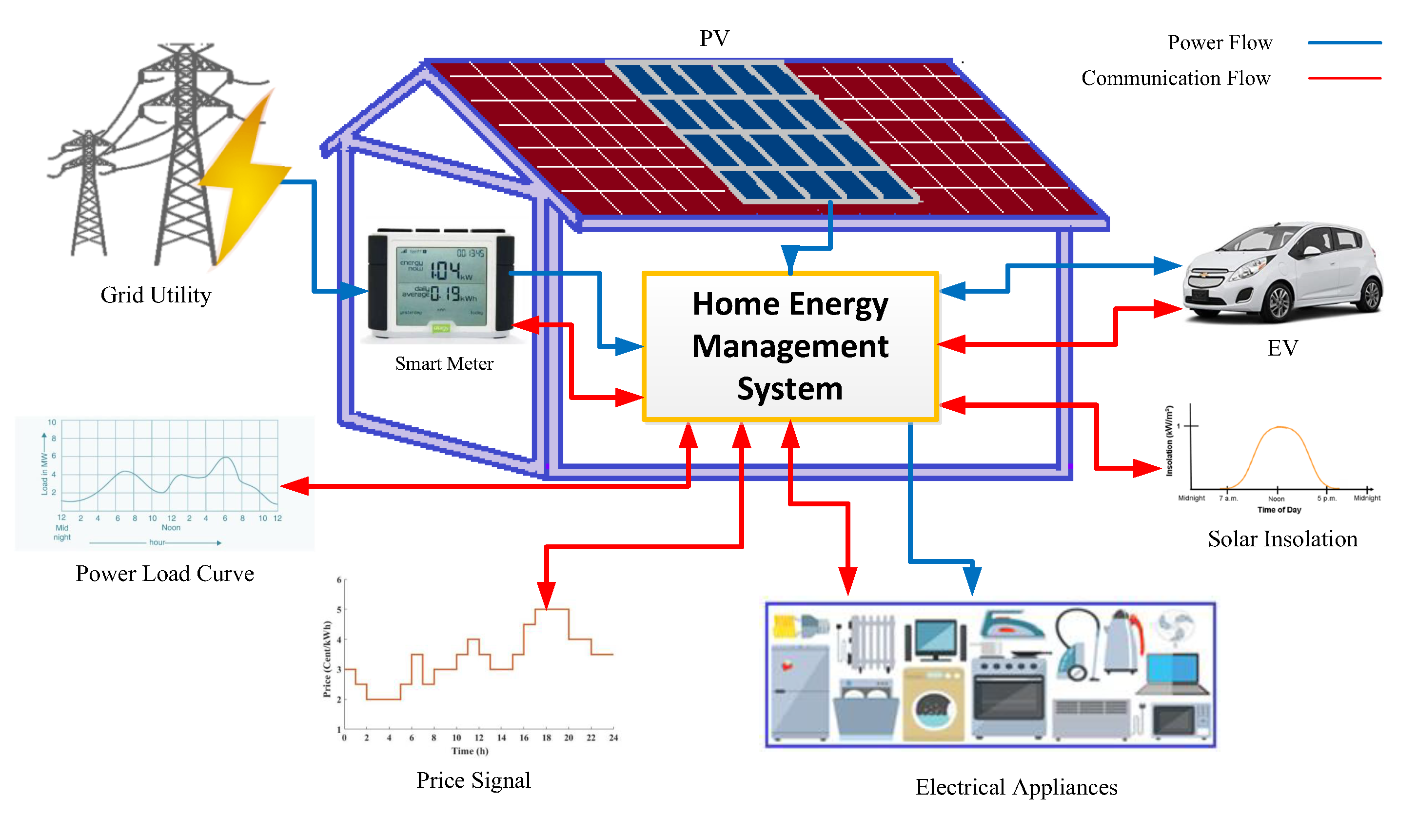
2.1. System Description

The schematic representation of the smart home is shown in Figure 1, which consists of household appliances, an electric vehicle (EV), a photovoltaic system (PV), daily load curve, daily solar insolation curve, daily price signal, grid utility, smart meter, and HEMS to manage and control the power flow among the utility grid, PV, household appliances, and EV. The smart home term in this study indicates that the home can provide two-way data communication and bidirectional power flow, which conforms to the smart grid concept.

2.2. System Modeling

2.2.1. Solar Photovoltaic Panel

The PV cells convert the sunlight (photons) into electrical energy through a photovoltaic effect. Then, the PV cells are connected in series or/and parallel to obtain the required value of the current and voltage at PV panel output [24]. The relation between the PV cell current $I_{pv}$ and voltage $V_{pv}$ can be represented in Equation (1) [25].

$$I_{pv}=I_{pc}-I_s\left[exp\left(\frac{q\left(V_{pv}+I_{pv}{R}_{se}\right)}{N_{s}nkT}\right)-1\right]-\left[\frac{V_{pv}-I_{pv}{R}_{se}}{R_{sh}}\right]$$

(1)

where $I_{pc}$ is the photovoltaic current (A), $I_s$ is the reverse saturation current of the cell (A), q is the electron charge ($1.602\times {10}^{-19}$ C), n is the ideality factor of the cell, k is the Boltzmann constant ($1.381\times {10}^{-23}$ J/k), T is the operating temperature (K), $N_s$ is the number of PV cells connected in series, $R_{se}$ is the series resistance of cell ($\Omega$), and $R_{sh}$ is the shunt resistance of cell ($\Omega$).

The photovoltaic sizing can be described by Equation (2) [26].

$$P{V}_{size}=\frac{L_d}{I_{d}d}\left(\mathrm{kW}\right)$$

(2)

where $L_d$ is the load to be covered by PV generation (kWh); $I_d$ is the peak sun shines hours, which is equal to 5.7 h per day in the target region; and d is the de-rating factor, which is assumed to be equal to 85%.

2.2.2. Electric Vehicle Modeling

Recently, lithium-ion batteries (Li-ion) have become commonly used in hybrid electric vehicles (HEVs) and electric vehicles (EVs) due to their high specific energy, high energy density, low rate of self-discharge, safety, high capability in the rate of charge and discharge, and long lifetime compared to other types of batteries [27]. Thus, in this study, we used an electric vehicle equipped with a Lithium-ion battery called Chevrolet Spark EV. The battery can be modeled and expressed as in Equation (3) [28].

$$V_{batt}=V_{oc}-R_i\times i_{batt}-V_D$$

(3)

where $V_{batt}$ is the terminal voltage of the battery (V); $V_{oc}$ is the battery open-circuit voltage (V); $R_i$ is the internal resistance ($\Omega$); $i_{batt}$ is the actual load current of the battery (A), which is negative at the charge and positive at discharge; and $V_D$ is the voltage drop due to polarization process (V) or polarization voltage.

The battery state of charge $SO{C}_{}$ (%) can be described by Equation (4), which is called the ampere-hour integral (Coulomb counting) [29].

$$SOC=SO{C}_0-\frac{1}{C_N}{\int }_{t_0}^t\eta i_{batt}dt$$

(4)

where $SO{C}_0$ (%) is the initial state of charge, $C_N$ is the rated capacity (Ah), and $\eta$ is the Coulomb efficiency.

According to EV battery capacity constraints, $SO{C}_{}$ will change due to charge from the grid and PV or discharge to feed the load. Then, $SO{C}_{}$ can be reformulated as defined in Equation (5).

$$SOC\left(t\right)=\left\{\begin{array}{cc}& SO{C}_0+\frac{1}{C_N}{\int }_{t_0}^t\eta \left(I_{PVEV}\left(t\right)+I_{GEV}\left(t\right)\right)dt\begin{array}{ccc}& if& charging\end{array}\\ & SO{C}_0-\frac{1}{C_N}{\int }_{t_0}^t\eta I_{EVL}\left(t\right)dt\begin{array}{cccccc}& & & & if& discharging\end{array}\end{array}\right.$$

(5)

where $SOC\left(t\right)$ represents the state of charge at the time t, $I_{PVEV}\left(t\right)$ represents the current from the PV-to-vehicle, $I_{GEV}\left(t\right)$ represents the current from the grid-to-vehicle, and $I_{EVL}\left(t\right)$ represent the current from the vehicle-to-load.

The deep charge/discharge cycles are minimized to extend the battery lifespan by setting a minimum and maximum limit for the state of charge [30]. Therefore, to prevent over-charge/discharge of the EV battery, $SOC\left(t\right)$ is set by following constraint as defined in Equation (6).

$$SO{C}_{min}\le SOC\left(t\right)\le SO{C}_{max}$$

(6)

where $SO{C}_{min}$ and $SO{C}_{max}$ are the minimum and maximum limit for the EV battery state of charge, respectively.

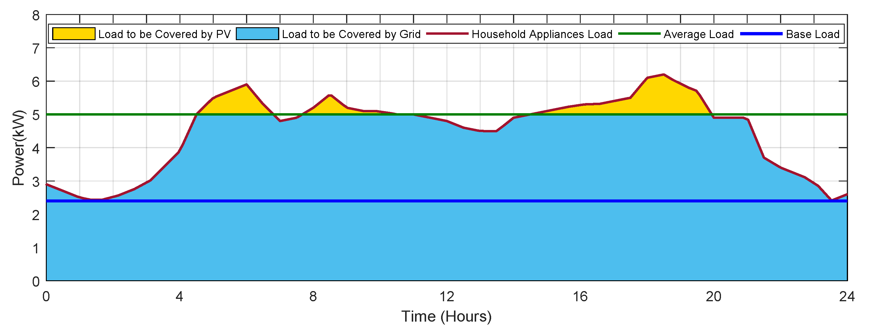
2.2.3. Household Load Demand

Consider a typical home with a group of appliances used in normal daily life at the house, such as CFL lamps, refrigerators, fans, air conditioners, televisions, cooking appliances, washing machines, etc. These devices consume electricity throughout the day, creating a daily load curve. The daily household appliances power demand can be calculated by the sum of all power consumed by the household appliances during the typical day, as defined in Equation (7) [31]. It is so hard to have a real load profile during the year time. Thus, the designers use the daily averages load for one day. Furthermore, other forecasting techniques can also be used, for example ANN, which can predict the load during a specific time [32]. The U.S. energy information administration (EIA) has collected hourly electricity consumption data in near-real-time from balancing authorities in the lower 48 states since 2015 [33]. They found that the household consumes a low amount of electricity during the night period, while there is high electricity consumption in the morning and evening. Therefore, the studied house is expected to consume high electricity during morning and evening, and low during the night, as depicted in Figure 2.

$$W_A=\sum _{t=1}^{24}{P}_L\left(t\right)$$

(7)

where $W_A$ represents the total energy consumed by the home appliances in the typical day (kWh), and $P_L\left(t\right)$ is the energy consumed by the home appliances in time slot t in (kW).

In this paper, it is assumed that the EV is a new load to be added to the studied home load. Thus, the average power of the studied home can be calculated as follows

$$P_{avg}=\frac{W_A+W_{ev}}{24}$$

(8)

where $P_{avg}$ is the average energy consumed by appliances and vehicle (kW) and $W_{ev}$ is the energy required for the electric vehicle trip (kWh).

The energy required for EV trip can be defined by Equation (9) [34].

$$W_{ev}={\eta }_{V}D$$

(9)

where ${\eta }_V$ is specific consumption (kWh/km) and D is the trip distance of the vehicle (km).

The typical household load curve can be divided into two parts: load above the average load line and the load under the average load line (Figure 2). In this study, if the sum of load above the average load line divided by (($I{}_d$) peak sun shines hours multiplied by (d) de-rating factor) is less than or equal to the base load of the home, the PV size will be scaled to cover the total load above the average load line. If the sum of load above the average load line divided by (($I{}_d$) peak sun shines hours multiplied by (d) de-rating factor) is greater than the base load of the home, the PV size will be scaled to be equal to the basic load of the home. Therefore, in this study, the electricity cannot be sold to the grid from the PV due to the PV generation being less than or equal to the home base load. The load to be covered by the PV generation can be calculated as follows.

$$L_d=\left\{\begin{array}{ccc}{\displaystyle \sum _{t=1}^{24}}((P_L\left(t\right)>P_{avg})-P_{avg})& if& \frac{{\displaystyle \sum _{t=1}^{24}}((P_L\left(t\right)>P_{avg})-P_{avg})}{I_{d}d}\le P_B\\ P_B{I}_{d}d& if& \frac{{\displaystyle \sum _{t=1}^{24}}((P_L\left(t\right)>P_{avg})-P_{avg})}{I_{d}d}>P_B\end{array}\right.$$

(10)

where $P_B$ is the base load of the home in kW (continuous load), which represents the minimum electrical demand amount needed during the period of 24-h time.

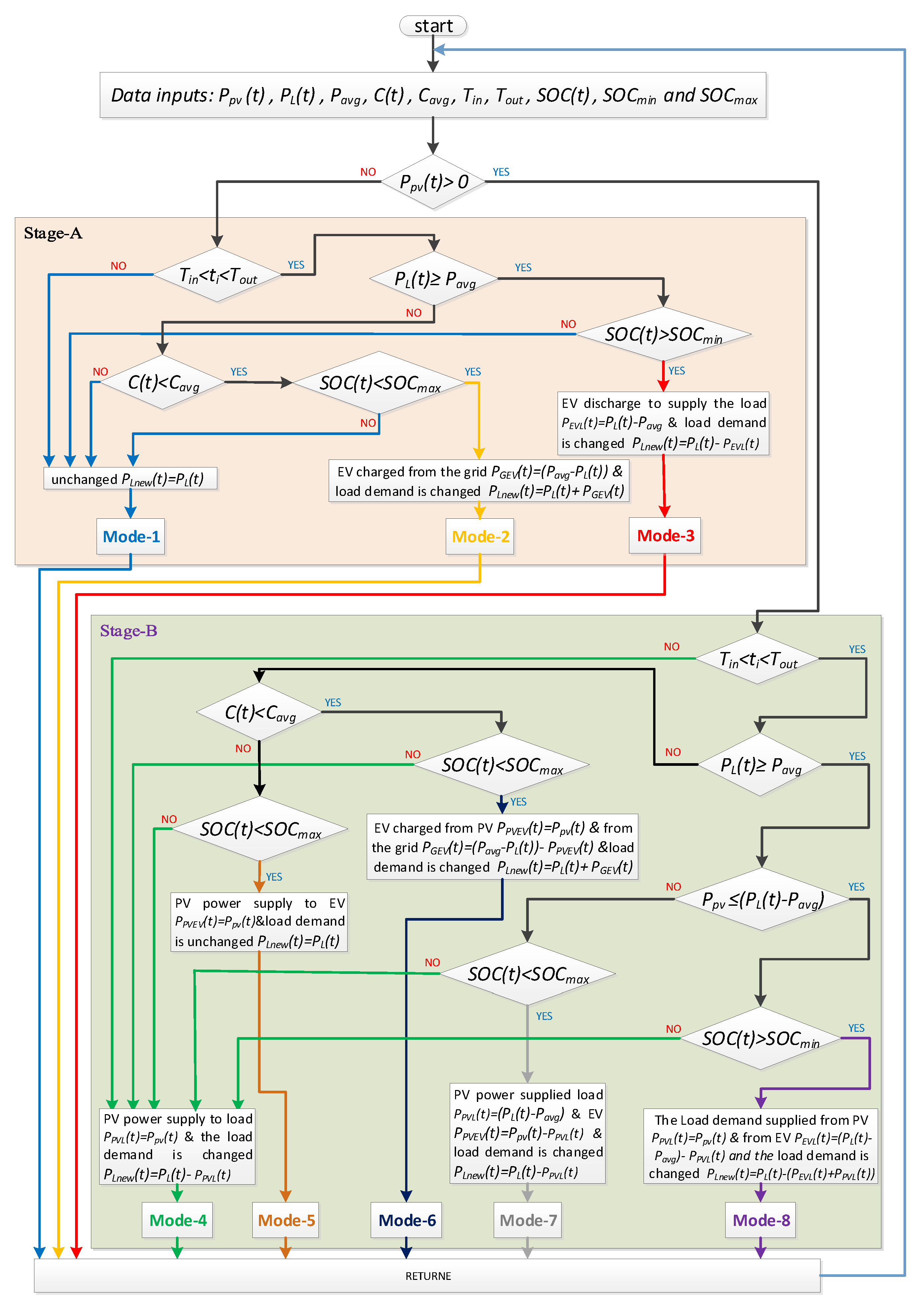
3. Proposed Energy Management Strategy

3.1. Proposed Energy Management Strategy for Smart Home Integrated with EV, and PV

Energy management strategies can play an important role in minimizing both electricity costs and the load power curve variance of the homes integrating PV and EV. In this context, this study investigates an energy management strategy for a smart home equipped with EV and PV. The proposed strategy illustrated in Figure 3 allows the power flow from grid-to-vehicle (G2V), PV-to–vehicle (PV2V), and vehicle-to-home (V2H) to minimize daily electricity cost and flattening the power load curve in the smart home. The proposed control strategy consists of two stages: Stage A, which operates in three operating modes according to the unavailability of PV power generation (PV power equals zero), and Stage B, which operates in five operating modes according to the availability of PV power generation (PV power greater than zero). The key function of this strategy is to control the EV charge and discharge times, control the amount of energy that must be absorbed from the grid and/or PV by EV, and the amount of energy that must be injected into the load demand from EV. That will help to reduce the electricity cost and maintain the load curve within the limits of the average load, as well as optimize energy use through achieving the following objectives:

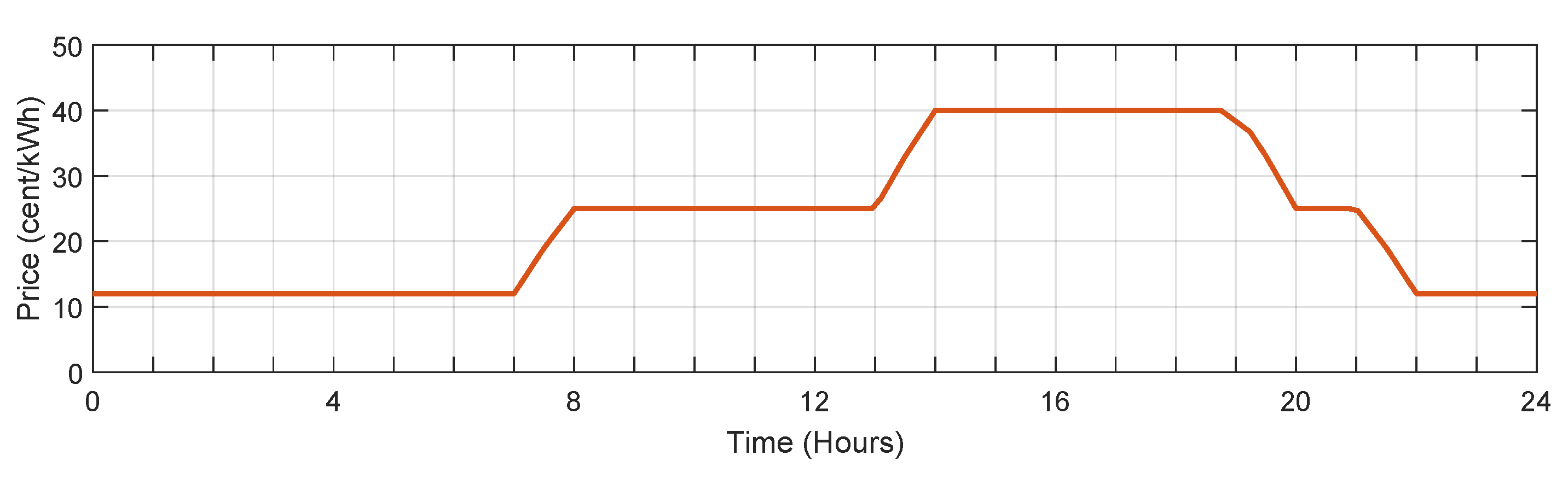
• Determine the low and high periods of electricity price.
• Detect the high and low electricity consumption periods in the studied home.
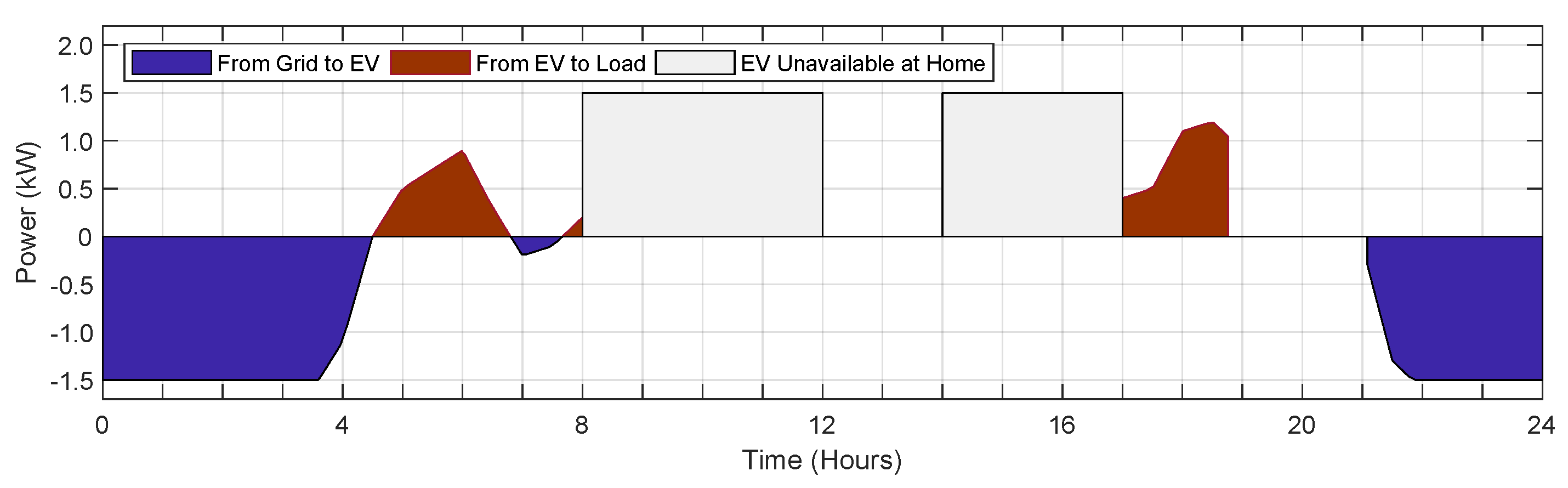
• Reduce the electricity cost and fill the valley thanks to charging EV from grid utility when the electricity price is low and electricity consumption is low simultaneously.
• Control the state-of-charge of electric vehicle battery to prevent the overcharge and over-discharge during charging and discharging, respectively.
• Determine the periods of a negative correlation among PV generation and the load that must be covered by PV generation to charge the electric vehicle from the surpluses PV generation.
• Reduce the peak load thanks to electric vehicle discharge to feed the load demand during the peak load period.

To realize the objectives mentioned above, the proposed strategy receives the following information as inputs: the daily photovoltaic power generation profile $P_{pv}\left(t\right)$, time-of-use price signal $C\left(t\right)$, daily load demand profile $P_L\left(t\right)$, average power load $P_{avg}$, average price signal $C_{avg}$, the arrival time of EV $T_{in}$, departure time of EV $T_{out}$, initial state-of-charge of the EV battery $SOC\left(t\right)$, maximum state-of-charge $SO{C}_{max}$, and minimum state-of-charge $SO{C}_{min}$. After that, the power is managed in two stages.

3.1.1. Stage A

When the PV power generation is equal to zero $P_{pv}\left(t\right)=0$, Stage A will operate to manage the power in three operating modes as follows:

Mode 1

In this mode, the EV will not charge/discharge. This mode is activated through activating one of four cases: (i) the EV is not at home; (ii) the EV is at home, the power load demand $P_L\left(t\right)$ is less than the average load $P_{avg}$, the electricity price $C\left(t\right)$ is less than the average price $C_{avg}$, and EV battery $SOC$ has reached its $SO{C}_{max}$ (EV battery fully charged); (iii) the EV is at home, power load demand $P_L\left(t\right)$ is less than average load $P_{avg}$ and electricity price $C\left(t\right)$ is greater than or equal to average price $C_{avg}$; or (iv) the EV is at home, power load demand $P_L\left(t\right)$ is greater than or equal to the average load $P_{avg}$ and EV $SOC$ has reached its $SO{C}_{min}$ (EV battery completely discharged). Therefore, the power load demand is unchanged as in Equation (11).

$$P_{Lnew}\left(t\right)=P_L\left(t\right)$$

(11)

where $P_{Lnew}\left(t\right)$ is the new amount of power consumed from the grid (kW).

Mode 2

This mode is detected if the EV is available at home, power load demand $P_L\left(t\right)$ is less than the average load $P_{avg}$, the electricity price $C\left(t\right)$ is less than the average price $C_{avg}$, and the EV battery $SO{C}_{}$ is less than $SO{C}_{max}$. Therefore, the EV is charged from the grid to fill the valley as defined by Equation (12), and the power load demand curve is changed according to Equation (13).

$$P_{GEV}\left(t\right)=-\left(P_L\left(t\right)-P_{avg}\right)$$

(12)

$$P_{Lnew}\left(t\right)=P_L\left(t\right)+P_{GEV}\left(t\right)$$

(13)

where $P_{GEV}\left(t\right)$ is the amount of power drawn from the grid to charge the electric vehicle (kW).

Mode 3

In this mode, the EV is at home, the power load demand $P_L\left(t\right)$ is greater than or equal to the average load $P_{avg}$, and the EV battery $SO{C}_{}$ is greater than $SO{C}_{min}$. Thus, the EV is discharged to shaving the peak load demand as calculated by Equation (14), and the power load demand curve is changed as defined in Equation (15).

$$P_{EVL}\left(t\right)=P_L\left(t\right)-P_{avg}$$

(14)

$$P_{Lnew}\left(t\right)=P_L\left(t\right)-P_{EVL}\left(t\right)$$

(15)

where $P_{EVL}\left(t\right)$ is the amount of power drawn from the electric vehicle to feed the load (kW).

3.1.2. Stage B

When the PV generation is higher than zero $P_{pv}\left(t\right)>0$, Stage B will operate to manage the power in five operating modes as follows:

Mode 4

In this mode, the EV will not charge/discharge, and the PV power is injected into load demand. This mode is activated through activating one of five cases as follows: (i) the EV is not at home; (ii) the EV is at home, power load demand $P_L\left(t\right)$ is less than the average load $P_{avg}$, electricity price $C\left(t\right)$ is less than the average price $C_{avg}$, and the EV battery $SOC$ has reached its $SO{C}_{max}$ (EV battery fully charged); (iii) the EV is at home, power load demand $P_L\left(t\right)$ is less than average load, electricity price $C\left(t\right)$ is greater than or equal to average price $C_{avg}$, and the EV battery $SOC$ has reached its $SO{C}_{max}$ (EV battery fully charged); (iv) the EV is at home, power load demand $P_L\left(t\right)$ is greater than or equal to average load $P_{avg}$, PV power $P_{pv}\left(t\right)$ greater than the power load demand minus the average load $P_L\left(t\right)-P_{avg}$ and the EV battery $SO{C}_{}$ has reached its $SO{C}_{max}$ (EV battery fully charged); or (v) the EV is at home, power load demand $P_L\left(t\right)$ is greater than or equal to the average load $P_{avg}$, PV power $P_{pv}\left(t\right)$ less than or equal to the power load demand minus the average load $P_L\left(t\right)-P_{avg}$, and the EV battery $SO{C}_{}$ has reached its $SO{C}_{min}$ (EV battery completely discharged). Therefore, the PV power is supplied to load demand as in Equation (16), and the power load demand curve is changed according to Equation (17).

$$P_{PVL}\left(t\right)=P_{pv}\left(t\right)$$

(16)

$$P_{Lnew}\left(t\right)=P_L\left(t\right)-P_{PVL}\left(t\right)$$

(17)

where $P_{PVL}\left(t\right)$ is the amount of power drawn from the PV to feed the load (kW).

Mode 5

In this mode, the EV is at home, the power load demand $P_L\left(t\right)$ is less than the average load $P_{avg}$, the electricity price $C\left(t\right)$ is greater than or equal to the average price $C_{avg}$, and the EV battery $SOC$ is less than $SO{C}_{max}$. Therefore, the EV is charged from the PV only due to the high electricity price, it can be expressed by Equation (18). The power load demand is unchanged according to Equation (11).

$$P_{PVEV}\left(t\right)=P_{pv}\left(t\right)$$

(18)

where $P_{PVEV}\left(t\right)$ is the amount of power drawn from the PV to charge the electric vehicle (kW).

Mode 6

This mode is operated if the EV is at home, power load demand $P_L\left(t\right)$ is less than the average load $P_{avg}$, the electricity price $C\left(t\right)$ is less than the average price $C_{avg}$, and EV battery $SOC$ is less than $SO{C}_{max}$. In this case, the EV should be charged from the grid and PV to fill the valley and transfer the PV to peak hours. The modified load demand, power flow from PV-to-vehicle, and grid-to-vehicle are expressed by Equations (13), (19) and (20), respectively.

$$P_{PVEV}\left(t\right)=P_{pv}\left(t\right)$$

(19)

$$P_{GEV}\left(t\right)=-\left(P_L\left(t\right)-P_{avg}\right)-P_{PVEV}\left(t\right)$$

(20)

Mode 7

Mode 7 is activated when the EV is available at home, power load demand $P_L\left(t\right)$ is greater than or equal to the average load $P_{avg}$, PV power $P_{pv}\left(t\right)$ is greater than power load demand minus the average load $P_L\left(t\right)-P_{avg}$, and the EV battery $SOC$ is less than $SO{C}_{max}$. In this mode, load demand and EV are fed from PV power. The power flow from PV-to-load, PV-to-vehicle, and modified power load are expressed as in Equations (21)–(23), respectively.

$$P_{PVL}\left(t\right)=P_L\left(t\right)-P_{avg}$$

(21)

$$P_{PVEV}\left(t\right)=P_{pv}\left(t\right)-P_{PVL}$$

(22)

$$P_{Lnew}\left(t\right)=P_L\left(t\right)-P_{PVL}$$

(23)

Mode 8

Mode 8 is selected when the EV is at home, power load demand $P_L\left(t\right)$ is greater than or equal to the average load $P_{avg}$, PV power $P_{pv}\left(t\right)$ is less than or equal to power load demand minus the average load $P_L\left(t\right)-P_{avg}$, and the EV battery $SOC$ is greater than $SO{C}_{min}$. In this mode, the EV is discharged to feed the load demand. The power flow from PV-to-load, vehicle-to-load, and modified power load are expressed as in Equations (24)–(26), respectively.

$$P_{PVL}\left(t\right)=P_{pv}\left(t\right)$$

(24)

$$P_{EVL}\left(t\right)=(P_L\left(t\right)-P_{avg})-P_{PVL}\left(t\right)$$

(25)

$$P_{Lnew}\left(t\right)=P_L\left(t\right)-(P_{EVL}\left(t\right)+P_{EVL}\left(t\right))$$

(26)

3.2. Proposed Energy Management Strategy for Smart Home Integrated with EV without PV

The proposed strategy for managing energy in the smart home equipped with EV and PV, shown in Figure 3, can also be employed to manage the energy in a smart home equipped with EV only. The proposed strategy receives the time-of-use price signal, daily load demand profile, average power load, average price signal, the arrival time of electric vehicle, departure time of electric vehicle, initial state-of-charge, the state-of-charge of the electric vehicle battery, maximum state-of-charge, and minimum state-of-charge as inputs. Then, the power is managed in Stage A of proposed strategy throughout the day, which operates in the first three modes only, as explained in Section 3.1.1.

4. Economic Analysis

In this section, three different cases are considered for a cost-benefit analysis to measure the profitability of proposed energy management strategy (EMS) for smart home includes PV and EV.

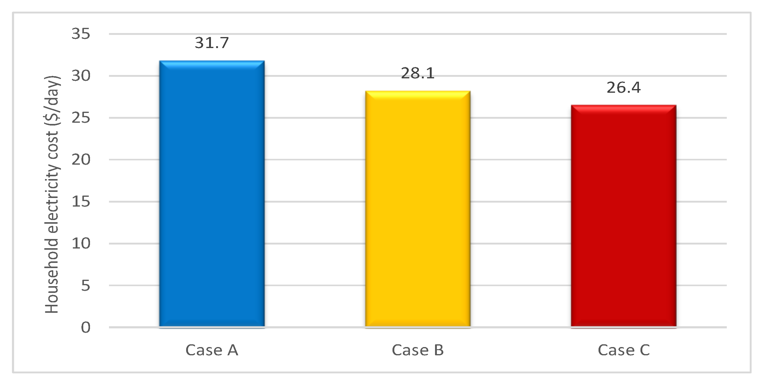
4.1. Case A: Home Equipped with EV and without EMS

In this case, the grid supplies the load demand, and the EV is considered as an electrical load at home, which is charged from the grid in the uncontrolled regime. Therefore, the total daily electricity costs can be calculated as follows.

$$C_{total}^A=\sum _{t=1}^{24}{P}_L\left(t\right)C\left(t\right)+\sum _{t=1}^{24}{P}_{GEV}\left(t\right)C\left(t\right)$$

(27)

where $C_{total}^A$ is the total daily electricity cost of Case A in $/day and $C\left(t\right)$ is the electricity price in $/kWh.

4.2. Case B: Home Equipped with EV and EMS

In this case, the EV is considered as energy storage. The energy is stored by charging the EV at off-peak period associated with a low price, and the V2H mode is used to supply the load at peak period, which contributes to reducing the total daily electricity costs. Thus, the equations obtained when the proposed strategy is employed to manage the energy in a smart home equipped with EV and without PV, as discussed in Section 3.2, were used to calculate the total daily electricity cost at home as follows.

$$C_{total}^B=\sum _{t=1}^{24}{P}_L\left(t\right)C\left(t\right)+\sum _{t=1}^{24}{P}_{GEV}\left(t\right)C\left(t\right)-\sum _{t=1}^{24}{P}_{EVL}\left(t\right)C\left(t\right)$$

(28)

where $C_{total}^B$ is the total daily electricity cost in $/day.

4.3. Case C: Home Equipped with EV, PV, and EMS

In this case, household Load demand is fed from the grid and PV beside EV through V2H mode. The EV is charged from the grid at the off-peak period associated with a low price and charged from the PV when the PV power is greater than the power load that required to be covered by PV power. Moreover, the EV discharges to feed the load during peak period, which will contribute to minimizing the total daily electricity costs. Thus, the equations obtained when the proposed strategy is employed to manage the energy in a smart home equipped with EV and PV, as discussed in Section 3.1, were used to calculate the total daily electricity cost at home as follows.

$$\begin{array}{cc}{C}_{total}^C& ={\displaystyle \sum _{t=1}^{24}}{P}_L\left(t\right)C\left(t\right)+{\displaystyle \sum _{t=1}^{24}}{P}_{GEV}\left(t\right)C\left(t\right)+P{V}_C^{day}-{\displaystyle \sum _{t=1}^{24}}{P}_{PVL}\left(t\right)C\left(t\right)-{\displaystyle \sum _{t=1}^{24}}{P}_{PVEV}\left(t\right)C\left(t\right)\hfill \\ & -{\displaystyle \sum _{t=1}^{24}}{P}_{EVL}\left(t\right)C\left(t\right)\hfill \end{array}$$

(29)

where $C_{total}^C$ is the total daily electricity cost in $/day and $P{V}_C^{day}$ is the PV installation cost per day in $/day.

The total PV cost includes the total capital cost and operational and maintenance costs, which can be represented by Equation (30) [35].

$$P{V}_{TC}=P{V}_{cap}+P{V}_{om}$$

(30)

where $P{V}_{TC}$ is the total PV cost in $/kW; $P{V}_{cap}$ is the total PV capital cost in $/kW, which includes system hardware (module price, inverter price, electrical BOS, and structural BOS), direct labor (electrical, mechanical, and general construction), indirect labor (design, engineering, and permitting), supply chain, overhead, and margin; and $P{V}_{om}$ is the operational and maintenance cost in $/kW-year and also includes the inverter replacement cost.

The annual cost concept is used to convert the non-annually PV capital cost to annually PV capital cost as in Equation (31) [35].

$$P{V}_{capann}=P{V}_{cap}\frac{r\times {\left(1+r\right)}^N}{{\left(1+r\right)}^N-1}$$

(31)

where $P{V}_{capann}$ is the annual PV capital cost in $/kW-year, r is the annual interest rate in percent, and N is the lifetime of the system in years.

Then, the total PV cost becomes annually as described by Equation (32).

$$P{V}_{TCann}=P{V}_{capann}+P{V}_{om}$$

(32)

where $P{V}_{TCann}$ represent the annually total PV installation cost in $/kW-year.

In this paper, the objective is to reduce electricity costs within 24 h or minimize total daily electricity costs at home, so the annual cost of solar photovoltaic must be converted into a daily cost to be combined with the other daily costs. The annual cost $P{V}_{TCann}$ is converted into daily cost $P{V}_C^{day}$ as expressed by Equation (33) [36].

$$P{V}_C^{day}=\frac{P{V}_{TCann}\times R_c}{365}$$

(33)

where $R_C$ represent the rated capacity of the PV system in kW.

5. Results and Discussion

The simulation was carried out to verify the performance and effectiveness of proposed strategy regarding the cost reduction and flatness of the load demand curve. In this study, the computerized horizon is set to 24 h. Solar data are taken from [37], which provides the solar irradiation and temperature data from 1981 up to date of accessed on 1 August 2020. For simplicity, the solar data were used over the past five years to evaluate the average output profiles, which can be predicted as in Figure 4.

Figure 5 depicts the real-time pricing signals [38], which is based on the residential TOU rates of Southern California Edison (SCE). This figure depicts the electricity price curve with Time-of-use in differentiated periods, in the range 12–40 cents/kWh, with an average price of 24 cents/kWh, which was calculated by summation of the electricity price during the day and dividing it by 24 h in this study. It motivates the homeowners to charge their electric vehicle in the off-peak period (cheap electricity price) and the EV battery discharge to feed load demand in the peak period to achieve economic benefits.

The EV parameter settings are presented in

Table 1. EV parameters.

Parameter	Value
EV battery capacity	19 kWh
$SO{C}_{\max }$	90%
$SO{C}_{\min }$	20%
$SO{C}_{\mathrm{in}}$	50%
Energy required for EV trip	9.2 kWh
Maximum power limit	1.5 kW
Minimum power limit	−1.5 kW
Leaving times	8:00, 14:00
Arrival times	12:00, 17:00
Vehicle efficiency ${\eta }_V$	14 kWh/100 km

. The most suitable level for charging the electric vehicle at home is 1.5–3 kW [39]. In this study, the EV daily travel distance is considered the same as the average daily driving in the U.S. according to the U.S. department of transportation, the average daily driving in the U.S. is 40 miles [40].

Moreover, it is assumed that the EV leaves home at 8:00 and arrives home at 12:00, and leaves home for the second time at 14:00 and arrives home at 17:00. The economic parameters associated with the PV system used in this study are presented in

Table 2. PV parameters.

Parameter	Value	Value After Tax Credit
lifetime	25	-
PV Rated power	1 kW	-
Capital cost	2830 $/kW	2094.2 $/kW
O and M cost	22 $/KW (per year)	22 $/Kw (per year)
Interest rate	4.8%	-

. In the first quarter of 2020, the total capital cost of the U.S photovoltaic system decreased to $2.83 /watt in the residential sector [41]. While the solar Investment Tax Credit (ITC) in the residential sector represents 26% of the total capital cost for projects that started in 2020 [42], the operational and maintenance cost and interest rate were taken from [43].

Figure 6 illustrates different eight modes when the proposed strategy is used to manage the energy in a smart home includes PV and EV. Modes 1–3 indicate that there is no available PV power, and thus the strategy works in Stage A. Modes 4–8 indicate that there is available PV power, and thus the strategy works in Stage B.

As shown in Figure 6, the system is operated in Stage A during the time intervals 00:00–06:00 and 18:30–24:00, while, during the time interval 06:00–18:30, the system is operated in Stage B.

Figure 7 explains different modes when the proposed strategy is used to control the energy in a smart home equipped with EV without PV. Figure 7 shows that the system is operated in Modes 1, 2, and 3 during the whole day, which means that the system is operated in Stage A only.

Figure 8 and Figure 9 show an electric vehicle battery state-of-charge curve when the proposed strategy is used to manage the energy in a smart home equipped with EV and PV and a smart home equipped with EV without PV, respectively. Figure 8 and Figure 9 confirm that the battery is in charging and discharging modes, in addition to proving that the state-of-charge is within the upper and lower limits during charging and discharging operations.

Figure 10 shows the electric vehicle power curve when the proposed strategy is used to control the energy in a smart home equipped with EV and PV. The negative power in periods 00:00–04:30 and 21:06–24:00 indicates that the EV is charged from the grid. The negative powers in the period 06:48–07:38 indicate that the EV is charged from the grid and PV. The negative powers in periods 06:43–06:48, 07:38–08:00, and 12:00–14:00 indicate that the EV is charged from PV. The positive powers in periods 04:30–06:43 and 17:00–19:55 indicate that the EV is discharged to feed the load. Periods 08:00–12:00 and 14:00–17:00 indicate that the EV is outside the home, thus the EV is not charged or discharged. Furthermore, the no change in the EV power curve in the period 19:55–21:06 indicates that the power load demand is less than the average load, and the electricity price is greater than or equal to the average price, so the EV is not charged or discharged.

Figure 11 shows the electric vehicle power curve when the proposed strategy is used for managing the energy in a smart home equipped with EV without PV. The negative powers in periods 00:00–04:30, 06:48–07:38, and 21:06–24:00 indicate that the EV is charged from the grid. The positive powers in periods 04:30–06:48, 07:38–08:00, and 17:00–18:45 indicate that the EV is discharged to feed the load. The time intervals 08:00–12:00 and 14:00–17:00 indicate that the EV is outside the home. No change in the EV power curve in periods 12:00–14:00 and 19:55–21:06 indicates that the power load demand is less than the average load, and the electricity price is greater than or equal to the average price, so the EV is not charged. The no change in the EV power curve in period 18:45–19:55 indicates that the power load demand is greater than or equal to the average load, but the EV battery $SOC$ has reached its $SO{C}_{min}$, so the EV is not discharged to feed the load.

Figure 12 displays power load curve without the EMS, the power load curve with EV and EMS, and the power load curve with EV, PV, and EMS. Figure 12 shows that the power load curve is flattened in the cases of power load curve with EV and EMS and with EV, PV, and EMS compared to the power load curve without the EMS. However, it is worth noticing that, in the case of using the proposed strategy for managing the energy in the smart home that includes EV and PV, the power load curve is smoother than the case in which the proposed strategy is used to manage the energy in the smart home that includes EV but not PV.

The household daily electricity cost is calculated in the three cases mentioned in Section 4. The daily household electricity cost of the three cases are presented in Figure 13. Figure 13 shows that the daily electricity cost is decreased in both Cases B and C compared to Case A. However, it is noticed that the daily electricity cost in Case C is less than the daily electricity cost in Case B, due to the use of PV in Case C.

The proposed strategy was compared with other strategies in the existing literature [17,21]. Authors in [17] presented an algorithm for controlling the charging/discharging of EVs in a home that focused on flattening the load curve depending on the daily load curve of household appliances only without taking into account time-varying electricity price. The control algorithm focused on reducing grid stress only and ignored the cost reduction for the homeowner. Authors in [21] introduced a control model based on stochastic optimization in the smart home with PV and EV that focused on reduce consumer energy charges while the flattening of the load curve was ignored. It is worth noting that all the aspects that were not covered in [17,21] are considered in this study.

6. Conclusions

In this study, an energy management strategy for a smart home that integrates EV and PV was proposed to minimize the household electricity costs and flatten the household power load curve. Eight different modes of the energy management strategy were developed, divided into two stages: Stage A, which operates in three modes depending on the unavailability of PV generation (i.e., PV power is equal to zero), and Stage B, which operates in five modes depending on the availability of PV power (i.e., PV power is greater than zero). EV parameters, time-of-use pricing, time-varying household power demand, and PV generation profile were used as inputs to the proposed strategy to ensure that both electricity costs and the load power curve variance were minimized while satisfying the system power requirements.

The corresponding simulation results show that, by using the proposed energy management strategy in a smart household containing EV with/without PV, the power load curve is flattened compared to the power load curve without using the proposed energy management strategy. Furthermore, the daily electricity costs were analyzed for the smart home integrated EV with/without PV generation under the proposed strategy, compared to a smart home equipped with EV and without PV generation under the regime of uncontrolled EV charging. It was found that the proposed control strategy can bring significant economic benefits to the homeowner, where the daily electricity costs were reduced from $ 32.7/day to $ 28.1/day through using the proposed strategy for the smart home equipped with EV without PV and to $ 26.4/day by using the proposed strategy for the smart home equipped with EV and PV.

Finally, it can be concluded that the proposed strategy for the smart home with EV and PV provides better results than the smart home with EV and without PV in terms of electricity costs reduction and power load profile flattening.

References

1. Liu, K.; Wang, Q.; Luo, Z.; Zhao, X.; Su, S.; Zhang, X. Planning Mechanism Design and Benefit Analysis of Electric Energy Substitution: A Case Study of Tobacco Industry in Yunnan Province, China. IEEE Access 2020, 8, 12867–12883. [Google Scholar] [CrossRef]
2. Savio, D.A.; Juliet, V.A.; Chokkalingam, B.; Padmanaban, S.; Holm-Nielsen, J.B.; Blaabjerg, F. Photovoltaic integrated hybridmicrogrid structured electric vehicle charging station and its energymanagement approach. Energies 2019, 12, 168. [Google Scholar] [CrossRef] [Green Version]
3. Sinsel, S.R.; Riemke, R.L.; Hoffmann, V.H. Challenges and solution technologies for the integration of variable renewable energy sources—A review. Renew. Energy 2020, 145, 2271–2285. [Google Scholar] [CrossRef]
4. Kemmler, T.; Thomas, B. Design ofHeat-Pump Systems for Single-and Multi-Family Houses using a Heuristic Scheduling for the Optimization of PV Self-Consumption. Energies 2020, 13, 1118. [Google Scholar] [CrossRef] [Green Version]
5. Kapustin, N.O.; Grushevenko, D.A. Long-term electric vehicles outlook and their potential impact on electric grid. Energy Policy 2020, 137, 111103. [Google Scholar] [CrossRef]
6. Luthander, R.; Shepero, M.; Munkhammar, J.; Widen, J. Photovoltaics and opportunistic electric vehicle charging in the power system—A case study on a Swedish distribution grid. IET Renew. Power Gener. 2019, 13, 710–716. [Google Scholar] [CrossRef] [Green Version]
7. Wi, Y.M.; Lee, J.U.; Joo, S.K. Electric vehicle charging method for smart homes/buildings with a photovoltaic system. IEEE Trans. Consum. Electron. 2013, 59, 323–328. [Google Scholar] [CrossRef]
8. Tarroja, B.; Eichman, J.D.; Zhang, L.; Brown, T.M.; Samuelsen, S. The effectiveness of plug-in hybrid electric vehicles and renewable power in support of holistic environmental goals: Part 2-Design and operation implications for load-balancing resources on the electric grid. J. Power Sources 2015, 278, 782–793. [Google Scholar] [CrossRef]
9. Lakshmi, G.S.; Rubanenko, O.; Hunko, I. Renewable Energy Generation and Impacts on E-Mobility. In Proceedings of the Journal of Physics: Conference Series, International Conference on Computer and Electrical Engineering, TU Delft, The Netherlands, 6–8 November 2019; Volume 1457, p. 012009. [Google Scholar]
10. Daki, H.; El Hannani, A.; Aqqal, A.; Haidine, A.; Dahbi, A. Big Data management in smart grid: Concepts, requirements and implementation. J. Big Data 2017, 4, 1–19. [Google Scholar] [CrossRef] [Green Version]
11. Shakeri, M.; Shayestegan, M.; Abunima, H.; Reza, S.S.; Akhtaruzzaman, M.; Alamoud, A.R.M.; Sopian, K.; Amin, N. An intelligent system architecture in home energy management systems (HEMS) for efficient demand response in smart grid. Energy Build. 2017, 138, 154–164. [Google Scholar] [CrossRef]
12. Leitao, J.; Gil, P.; Ribeiro, B.; Cardoso, A. A survey on home energy management. IEEE Access 2020, 8, 5699–5722. [Google Scholar] [CrossRef]
13. Olsen, D.J.; Sarker, M.R.; Ortega-Vazquez, M.A. Optimal penetration of home energy management systems in distribution networks considering transformer aging. IEEE Trans. Smart Grid 2016, 9, 3330–3340. [Google Scholar] [CrossRef]
14. Luo, F.; Ranzi, G.; Kong, W.; Dong, Z.Y.; Wang, F. Coordinated residential energy resource scheduling with vehicle-to-home and high photovoltaic penetrations. IET Renew. Power Gener. 2018, 12, 625–632. [Google Scholar] [CrossRef]
15. Datta, U.; Kalam, A.; Shi, J. Electric vehicle (EV) in home energy management to reduce daily electricity costs of residential customer. J. Sci. Ind. Res. 2018, 77, 559–565. [Google Scholar]
16. Wu, X.; Hu, X.; Yin, X.; Moura, S.J. Stochastic optimal energy management of smart home with PEV energy storage. IEEE Trans. Smart Grid 2016, 9, 2065–2075. [Google Scholar] [CrossRef]
17. Khemakhem, S.; Rekik, M.; Krichen, L. A flexible control strategy of plug-in electric vehicles operating in seven modes for smoothing load power curves in smart grid. Energy 2017, 118, 197–208. [Google Scholar] [CrossRef]
18. Khemakhem, S.; Rekik, M.; Krichen, L. Double layer home energy supervision strategies based on demand response and plug-in electric vehicle control for flattening power load curves in a smart grid. Energy 2019, 167, 312–324. [Google Scholar] [CrossRef]
19. Rana, R.; Prakash, S.; Mishra, S. Energy Management of Electric Vehicle Integrated Home in a Time-of-Day Regime. IEEE Trans. Transp. Electrif. 2018, 4, 804–816. [Google Scholar] [CrossRef]
20. Erdinc, O.; Paterakis, N.G.; Mendes, T.D.; Bakirtzis, A.G.; Catalao, J.P. Smart household operation considering bi-directional EV and ESS utilization by real-time pricing-based DR. IEEE Trans. Smart Grid 2014, 6, 1281–1291. [Google Scholar] [CrossRef]
21. Wu, X.; Hu, X.; Moura, S.; Yin, X.; Pickert, V. Stochastic control of smart home energy management with plug-in electric vehicle battery energy storage and photovoltaic array. J. Power Sources 2016, 333, 203–212. [Google Scholar] [CrossRef] [Green Version]
22. Aznavi, S.; Fajri, P.; Asrari, A.; Harirchi, F. Realistic and intelligent management of connected storage devices in future smart homes considering energy price tag. IEEE Trans. Ind. Appl. 2019, 56, 1679–1689. [Google Scholar] [CrossRef]
23. Lee, S.; Choi, D.H. Energy Management of Smart Home with Home Appliances, Energy Storage System and Electric Vehicle: A Hierarchical Deep Reinforcement Learning Approach. Sensors 2020, 20, 2157. [Google Scholar] [CrossRef] [PubMed] [Green Version]
24. Krismadinata, N.A.R.; Ping, H.W.; Selvaraj, J. Photovoltaic module modeling using Simulink/Matlab. Procedia Environ. Sci. 2013, 17, 537–546. [Google Scholar] [CrossRef] [Green Version]
25. Laudani, A.; Fulginei, F.R.; Salvini, A. Identification of the one-diode model for photovoltaic modules from datasheet values. Sol. Energy 2014, 108, 432–446. [Google Scholar] [CrossRef]
26. Hossain, C.A.; Chowdhury, N.; Longo, M.; Yaici, W. System and cost analysis of stand-alone solar home system applied to a developing country. Sustainability 2019, 11, 1403. [Google Scholar] [CrossRef] [Green Version]
27. Wang, Q.; Jiang, B.; Li, B.; Yan, Y. A critical review of thermal management models and solutions of lithium-ion batteries for the development of pure electric vehicles. Renew. Sustain. Energy Rev. 2016, 64, 106–128. [Google Scholar] [CrossRef]
28. Zhu, R.; Duan, B.; Zhang, C.; Gong, S. Accurate lithium-ion battery modeling with inverse repeat binary sequence for electric vehicle applications. Appl. Energy 2019, 251, 113339. [Google Scholar] [CrossRef]
29. Lu, L.; Han, X.; Li, J.; Hua, J.; Ouyang, M. A review on the key issues for lithium-ion battery management in electric vehicles. J. Power Sources 2013, 226, 272–288. [Google Scholar] [CrossRef]
30. El-Sehiemy, R.A.; Hamida, M.A.; Mesbahi, T. Parameter identification and state-of-charge estimation for lithium-polymer battery cells using enhanced sunflower optimization algorithm. Int. J. Hydrog. Energy 2020, 45, 8833–8842. [Google Scholar] [CrossRef]
31. Saberi, K.; Pashaei-Didani, H.; Nourollahi, R.; Zare, K.; Nojavan, S. Optimal performance of CCHP based microgrid considering environmental issue in the presence of real time demand response. Sustain. Cities Soc. 2019, 45, 596–606. [Google Scholar] [CrossRef]
32. Khatib, T.; Mohamed, A.; Sopian, K. A review of photovoltaic systems size optimization techniques. Renew. Sustain. Energy Rev. 2013, 22, 454–465. [Google Scholar] [CrossRef]
33. U.S. Energy Information Administration-Hourly Electricity Consumption Varies Throughout the Day and across Seasons. 2020. Available online: https://www.eia.gov/todayinenergy/detail.php?id=42915 (accessed on 1 August 2020).
34. Fachrizal, R.; Munkhammar, J. Improved Photovoltaic Self-Consumption in Residential Buildings with Distributed and Centralized Smart Charging of Electric Vehicles. Energies 2020, 13, 1153. [Google Scholar] [CrossRef] [Green Version]
35. Singh, S.; Singh, M.; Kaushik, S.C. Feasibility study of an islanded microgrid in rural area consisting of PV, wind, biomass and battery energy storage system. Energy Convers. Manag. 2016, 128, 178–190. [Google Scholar] [CrossRef]
36. Chen, S.X.; Gooi, H.B.; Wang, M. Sizing of energy storage for microgrids. IEEE Trans. Smart Grid 2011, 3, 142–151. [Google Scholar] [CrossRef]
37. National Renewable Energy Laboratory. Available online: https://midcdmz.nrel.gov/ (accessed on 1 August 2020).
38. Ramdas, A.; McCabe, K.; Das, P.; Sigrin, B.O. California Time-of-Use (TOU) Transition: Effects on Distributed Wind and Solar Economic Potential; Technical Report No. NREL/TP-6A20-73147; National Renewable Energy Lab.(NREL): Golden, CO, USA, 2019.
39. Young, K.; Wang, C.; Strunz, K. Electric vehicle battery technologies. In Electric Vehicle Integration into Modern Power Networks; Springer: New York, NY, USA, 2013; pp. 15–56. [Google Scholar]
40. McGuckin, N.; Fucci, A. Summary of Travel Trends: 2017 National Household Travel Survey; Technical Report No. FHWA-PL-18-019; Federal Highway Administration, US Department of Transportation: Washington, DC, USA, 2018.
41. Solar Energy Industries Association—Solar Market Insight Report 2020 Q2. 2020. Available online: https://www.seia.org/research-resources/solar-market-insight-report-2020-q2 (accessed on 1 August 2020).
42. Solar Energy Industries Association. Available online: https://www.seia.org/initiatives/solar-investment-tax-credit-itc (accessed on 1 August 2020).
43. Fu, R.; Feldman, D.J.; Margolis, R.M. US Solar Photovoltaic System Cost Benchmark: Q1 2018 Technical Report No. NREL/TP-6A20-72399; National Renewable Energy Lab.(NREL): Golden, CO, USA, 2018.
Figure 1. Structure of smart home.
Energies 13 06387 g001
Figure 2. Hourly household appliances electricity consumption.
Energies 13 06387 g002
Figure 3. Proposed energy management strategy flowchart.
Energies 13 06387 g003
Figure 4. Hourly average solar Insolation.
Energies 13 06387 g004
Figure 5. Hourly electricity price signal.
Energies 13 06387 g005
Figure 6. Different operation modes achieved by the proposed strategy when used to manage the energy in a smart home equipped with PV and EV.
Energies 13 06387 g006
Figure 7. Different operation modes achieved by the proposed strategy when used to manage the energy in a smart home equipped with EV without PV.
Energies 13 06387 g007
Figure 8. State of charge curve of EV when the proposed strategy is used to managing the energy in a smart home equipped with PV and EV.
Energies 13 06387 g008
Figure 9. State of charge curve of EV when the proposed strategy is used to managing the energy in a smart home equipped with EV without PV.
Energies 13 06387 g009
Figure 10. EV charging and discharging power profile when the proposed strategy is used for managing the energy in a smart home equipped with EV and PV.
Energies 13 06387 g010
Figure 11. EV charging and discharging power profile when the proposed strategy was used for managing the energy in a smart home equipped with EV without PV.
Energies 13 06387 g011
Figure 12. Daily household Power load curve without EMS, daily household Power load curve with EV and EMS, and daily household Power load curve with EV, PV, and EMS.
Energies 13 06387 g012
Figure 13. The daily electricity cost of the household in three cases.
Energies 13 06387 g013