3.1. Reconstruction Performances of Rock Properties
The parameter size is examined with the comparison of typical fully-connected-layer-type (multi-layered-perceptron-type; MLP-type) autoencoder [
37,
38].
Table 2 shows the number of parameters used by a typical MLP-type autoencoder if we set the latent features used to be the same as those of our DCAE, i.e., the 1920 parameters that represent 4.3% of the input data (the original 44,460 three-dimensional spatial properties). Notwithstanding the fact that the details of designing the MLP-type autoencoder may differ according to the user’s purpose, the general architecture is configured; a symmetrical structure uses the node number set to 1/3 or more in the previous layer to prevent any excess information loss. The total number of parameters would be about 1.5 billion for the encoding and decoding processes and thereby it is not practical to train this kind of network from the viewpoint of computational efficiency.
Figure 4 explains the DCAE architecture in detail;
Figure 4a demonstrates the encoding process that reduces (38 × 45 × 13 × 2) dimensions to a (5 × 6 × 2 × 32) dimensional latent code, and
Figure 4b shows the decoding workflow to reconstruct spatial properties (permeability and porosity) that have the same dimensions as the original data (38 × 45 × 13 × 2). The latent features are significantly reduced in the input data, decreasing from 44,460 to 1920.
Table 3 and
Table 4 summarize the details of how our DCAE encodes and decodes the data. As shown in
Table 3 and
Table 4, the total number of parameters in the DCAE system is 2,303,466 (=1,864,992 + 438,474) which is only 0.155% of what a typical MLP-type autoencoder would need to use (refer to
Table 2). Our fully-convolutional network consists of 27 convolutional layers and 18 batch normalizations. The ‘Adam’ optimizer is chosen after testing Adam, RMSprop, Adamax, and Adagrad optimizers. The activation function is ‘ReLU (rectified linear unit)’ and the He normal initializer is used [
39,
40]. The loss function is based on the mean squared error. The normalization of the input image is carried out based on the maximum pixel value and thus all inputs range between 0 and 1.
Figure 5 depicts DCAE training performances; here, the training loss and the validation loss values are compared. The local fluctuation observed in the trajectory of the validation loss is caused by the learning rates being updating. Both losses decrease steadily and converge to the minimum loss near the 350th epoch. The computation time is also fast achieving a rate of approximately 1.92 s/epoch (AMD Ryzen Threadripper 3960× 24-cores 3.79 GHz; 128 Gb RAM; NVIDIA Geforce RTX 2080Ti). The trends in
Figure 5 confirm that DCAE-based feature extraction (dimensionality reduction) leads to stable convergence without overfitting while only incurring small computing costs and shows the efficiency of the DCAE architecture introduced in this study.
The DCAE reconstructs spatial properties reliably.
Table 5 summarizes the reconstruction performance in terms of R-squared, RMSE, and MAPE.
Figure 6 compares the mean and the standard deviation of the permeabilities from the original input and the reconstructed geo-models. For example, 22,230 (=38 × 45 × 13) permeability values are input; the DCAE reconstructed these for each geo-model, and thereby one mean and one standard deviation are evaluated for each geo-model. The DCAE training operation (for 500 geo-models) matches the mean permeability up to 0.999 for the R-squared value, 0.872 millidarcy for RMSE, and 0.18% for MAPE. The results for the mean permeability from the validation and test sets have slightly lower R-squared values than the training set, i.e., 0.997 for the validation set (50 geo-models) and 0.996 for the test set (50 geo-models), but these differences are small enough to confirm the reliability of the DCAE. The standard deviations of reconstructed permeabilities have slightly lower values than the original inputs, of which the reasons would be from the inevitable information loss during dimension compression. All performance metrics related to the standard deviations of the training, validation, and test sets show similar trends. The R-squared values of the standard deviations for permeabilities are 0.992 for the training set, 0.983 for validation, and 0.980 for the test set.
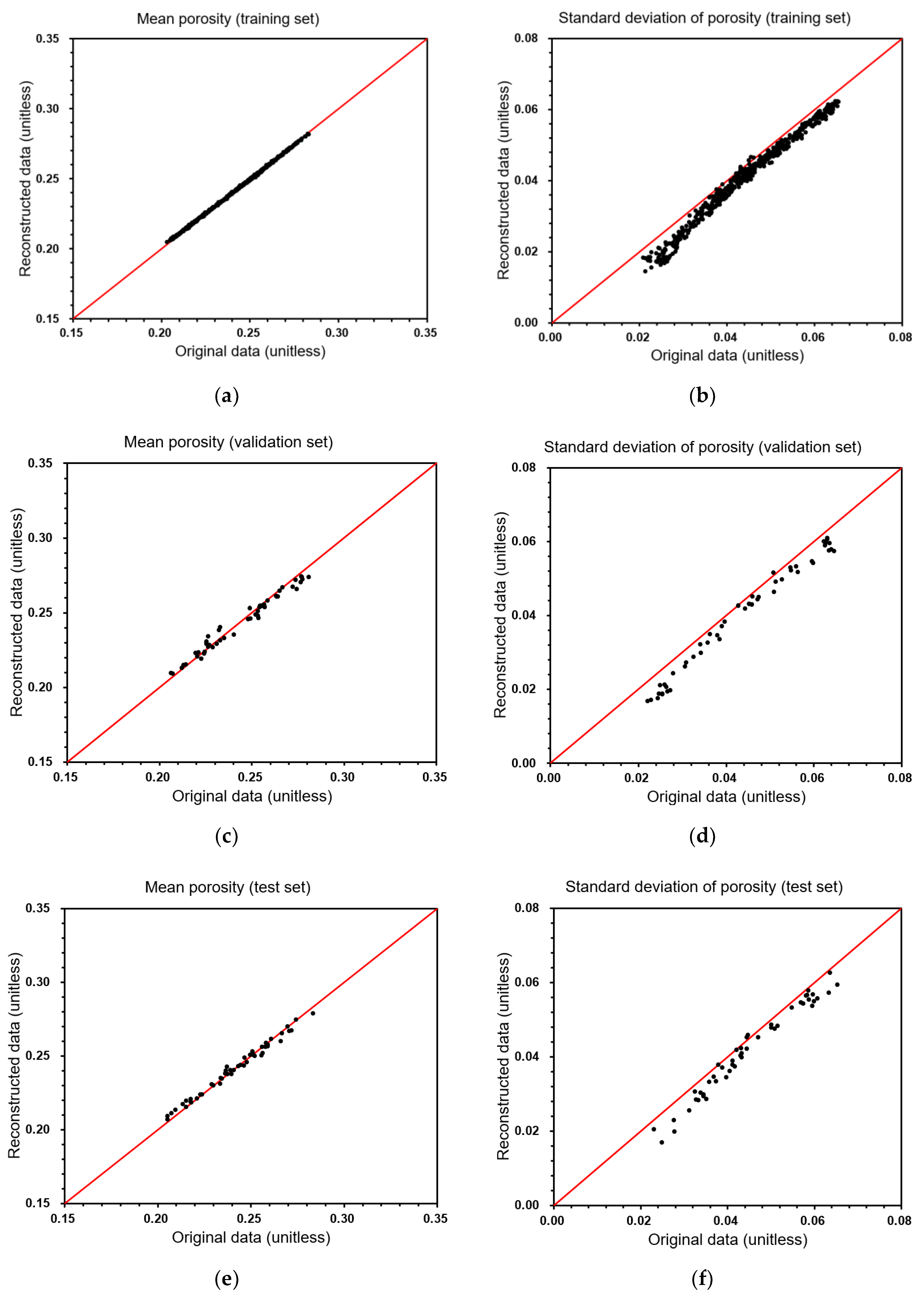
Figure 7 depicts a comparison of the porosities between the original input and the reconstructed data. In a similar way to the results already shown in
Figure 6, the porosity prediction is accurate and efficient. The R-squared values for mean porosity after reconstruction are 0.999 for the training set, 0.979 for the validation set, and 0.989 for the test set. The lowest R-squared value is 0.972 for the standard deviation of the porosities with the test set. Analyzing
Figure 6 and
Figure 7, as well as
Table 5, it is clear that the DCAE is able to extract latent features and then reconstruct the spatial properties accurately.
In short, after evaluating the performance of the DCAE-based feature extraction, it can be concluded that the developed architecture can reduce the number of parameters required for reconstruction to just 2,303,466 for both encoding and decoding operations, which is only 0.155% of what a typical symmetric-autoencoder would require. The extracted features are reliable, which is shown by the small errors and the high R-squared values after reconstructing the original spatial values. Another notable conclusion is that the DCAE can integrate different spatial properties within a single architecture and also regenerate both spatial values accurately from a statistical viewpoint. The results confirm that the developed DCAE-based feature extraction can be applied efficiently for upscaling and downscaling spatial properties.
3.2. Surrogate Estimation for CO2 Geological Sequestration
An adaptive surrogate model is constructed to estimate CO
2 sequestration as an alternative to time-consuming simulations.
Figure 8 and
Table 6 explain the detailed architecture of adaptive surrogate estimation using the features extracted from spatial data on permeability and porosity, the modeling parameters such as salinity and temperature, as well as the operating conditions such as the minimum well bottom hole pressure and the maximum CO
2 injection rates. The input dimensions are (5 × 6 × 2 × 36) while there are three outputs after global average pooling. The model consists of a fully-convolutional neural network but while we do not implement the fully-connected layers, seven convolutional layers and seven batch normalizations are included. The number of parameters used for the adaptive surrogate estimation is 348,239.
Figure 9 shows the training and validation losses with epochs. The
y-axis values are expressed as RMSE with units of million cubic meters to improve the understanding of training performances. The graph shows stable convergence and confirms that the model is efficient enough to converge to the final solutions without any remarkable fluctuations after 100 epochs. The computing time required is 0.09 s/epoch and no issues related to overfitting matters are experienced, and thus we can see that the surrogate model with the fully-convolutional network developed in this paper converges stably to the final optimality.
Figure 10 depicts the performances for estimating the output responses with the test set (50 geo-models), i.e., the structural trap amount (
Figure 10a), the dissolved trap amount (
Figure 10b), and the total CO
2 volume injected into the aquifer (
Figure 10c).
Table 7 summarizes the results of the indicators used to evaluate the prediction performance. The highest R-squared value, 0.989, is observed for predicting the dissolved trap amount; a possible reason for this would be assigning salinity and temperature as the input units that influence CO
2 dissolution. The heterogeneity of aquifer properties more strongly affects the structural trap amount and the total CO
2 injected volume. However, the MAPEs are lower than that of the dissolved trap amount, which is 3.02% as shown in
Table 7. Thus, we can conclude that both the spatial heterogeneity and operating conditions influence the predictability. A notable result is that the errors are less than 3.02% of the MAPE so that the adaptive surrogate estimation is accurate without the need for time-consuming physically-based simulations.
The large number of parameters involved in the deep-learning workflow cannot be free from ‘the curse of dimensionality’. The dimensionality reduction is essential to solve the following problems: convergence and computation efficiency. The high dimensions have sparse characteristics, the distance between training samples would be far, the extrapolation to forecast unknown values is unstable, and thus the overfitting and the poor convergence matters become more likely. In addition, the large number of operations, e.g., dot products between the kernel and the feature map, and the training parameters decrease the computational efficiency; the computing cost of adaptive surrogate estimation is 0.09 s/epoch. If analyzing the approximate computation time, the adaptive surrogate estimation requires 1005 s including the time for training over 500 epochs and estimating 50 test geo–models (=500 × (1.92 for DCAE + 0.09 for surrogate estimation); the prediction time is negligible. In contrast, the conventional flow simulations need 13,940 s to complete the 50 test geo–models(=278.8 × 50). Thus, the adaptive surrogate estimation can dramatically reduce the computational time required to approximately 7% of the time for the conventional flow simulation.
This study reduces the size of the feature map and convolutional operations required. In this way, an improvement of the computational efficiency is obtained. The methodology exploits the data integration within a single architecture unlike typical multimodal deep-learning approaches, and thus our method is able to successfully execute the reliable reconstruction of spatial properties as well as efficient dimensionality reduction.
An original part of the developed adaptive model in terms of methodology is that all inputs are integrally regarded as image channels from the initial stage of learning while typical multimodal models integrate the dataset within the flattened layers. Another key point is to use the fully-convolutional network and global average pooling instead of fully-connected layers, which is done to minimize the data loss without flattening the data to a one-dimensional array, and also to mitigate overfitting. Designing the proper hyper-parameters (such as the size of the feature map, the number of convolutional layers, kernel size, and the number of kernels, etc.) dominates the computational efforts, and thus the optimal designs that combine sub-sections of deep-learning will be challenging to reach the optimality of adaptive surrogate estimations. Notwithstanding that this paper shows successful estimation of three key results related to CO2 sequestration performance without using physically-based simulations, the spatiotemporal responses, e.g., saturation distribution and sequestration amount with time, need to be evaluated accurately in order to completely replace time-consuming subsurface flow simulations.


