The Environmental Efficiency Analysis Based on the Three-Step Method for Two-Stage Data Envelopment Analysis

Abstract

This paper suggests that the efficiency of a system (decision-making unit) and its subsystem cannot be properly measured using a two-stage data envelopment analysis (DEA) model either in cooperative or non-cooperative evaluation. Indeed, the existing methods subjectively determine the status of the subsystems in the whole system. The two-stage DEA models, either cooperative game or non-cooperative game, are used to analyze the environmental efficiency. However, when the actual relationship between the two subsystems is inconsistent with the subjective relationship assumptions, the overall efficiency of the system and the efficiency of each subsystem will be biased. The conventional two-stage DEA models require predetermining the relationship between the subsystems within the system based on the subjective judgment of the decision-maker. Based on this, this paper proposes a three-step method to solve the two-stage DEA. First, the position relation among subsystems is determined according to the optimal weights through the model. According to the status relationship among subsystems, the decision units are grouped, and the two-stage DEA model of cooperative game or non-cooperative game is used to analyze the efficiency in each group. This method reduces the subjectivity of decision making and analyzes the efficiency of each decision unit applying the most appropriate two-stage DEA model to find the source of inefficiency. Finally, this paper verifies the rationality and validity of the method by analyzing the water use efficiency of industrial systems in China. It is found that most regions in China value economic development more than environmental protection (as evidenced by the DEA weights). What is more, the method proposed by the paper can be generalized for any two-stage DEA problem.

1. Introduction

Energy and environmental issues are the big problems underpinning the development of the world and separate regions [1,2]. Data envelopment analysis (DEA) as a kind of non-parametric method of efficiency evaluation for decision-making units (DMU) has been widely used in the evaluation of the environmental efficiency [3]. For example, Zhou evaluates the environmental efficiency of 26 OECD countries by non-radial DEA [4]. When evaluating environmental efficiency, undesirable outputs are involved. The methods of dealing with undesirable outputs can be broadly divided into eight categories: curve measurement method [5], input processing method [6], data transformation method [7], directional distance function method based on the weak disposability [8], evaluation model based on relaxation variable (SBM model) [9], the evaluation model based on weak G disposability and material balance principle [10], by-production approach [11], and the non-radial efficiency measurement based on the natural and managerial disposability [12,13]. The latter three approaches are the latest developments in the field of environmental efficiency. These methods have their respective advantages and disadvantages; for example, the production process of the input method cannot reflect the real treatment, and the directional distance function method based on weak disposal does not conform to the thermal kinetic law [14]. When these methods evaluate environmental efficiency, they use DMU as a black box to analyze the environmental efficiency of each DMU. Sueyoshi and Goto [15] presented a review of applications of the DEA in an energy and environment context.

However, in practice, a production system (DMU) is often made up of different subsystems, each of which has its own inputs and outputs. If we analyze the environmental efficiency of each production system only from the “black box” angle, it is difficult to ascertain the reasons for the inefficiency of the production system. In recent years, the research on DEA is mainly focused on the evaluation of DMU with a complex internal structure. Two-stages of DEA and network DEA are proposed. Cook et al. review the two-stage DEA model and divided the existing methods into two-stages: cooperative game and non-cooperative game DEA [16]. Kao reviews the existing DEA network model and divided it into several types: independent model, system distance measurement model, and the measurement model based on the relaxation and game theory model [17]. Furthermore, he divides the structure of network DEA into seven kinds: that is, the basic two-stage structure, the generalized two-stage structure, the continuous structure, the parallel structure, the mixed structure, the hierarchical structure, and the dynamic structure. These models take full account of the relationship between the overall system efficiency and the efficiency of internal subsystems, but they do not consider undesirable outputs. Bian applied weak and strong disposition to undesirable output in different stages and proposed the SBM model. The efficiency analysis of a regional industrial system for China is conducted, but the relationship between the two subsystems in the model simply defines a connection, which cannot really reflect the relations among the two subsystems [18]. Taking into account the relationship between the two subsystems, Bian assumed that the economic development subsystem is in a leading position. According to the proposed two-stage DEA model of the non-cooperative game, the environmental efficiency analysis of the production system is conducted [19]. Chen, supplementing Bian’s research, proposed a two-stage DEA model based on cooperative game, arguing that the economic development subsystem and pollutant processing subsystem in the production system are equally important [20]. However, they subjectively determine the status of the two subsystems in the whole system, and the corresponding two-phase DEA model through cooperative game or non-cooperative game is used to analyze the environmental efficiency. However, when the actual status relationship between the two subsystems is inconsistent with the subjective status relationship, the overall efficiency of the system and the efficiency of each subsystem will be wrongly evaluated. Wang et al. propose a two-stage, network-based super data envelopment analysis (DEA) approach to investigate the overall efficiency and eco-efficiency of the sub-stages in China’s industrial system, including the production and three pollutant treatment stages [21]. Zeng et al. proposed a two-stage DEA linear model to evaluate environmental efficiency, which adopts the material balance principle and meanwhile considers both the production stage and end-of-pipe abatement stage [22]. Zhao et al. developed a theoretical framework within the data envelopment analysis context to examine the efficiency of sustainable development systems composed of an economic and environmental subsystem and a social subsystem under an independently parallel setting [23]. Lin et al. proposed an extended DEA model, which combines global benchmark technology, directional distance function, and a bootstrapping approach to investigate the dynamic trends of regional eco-efficiency in China [24].

So far, there is no research that works on the two-stage DEA with objective determination of the relationship between the subsystems. Drawing inspiration from the group boundary method [25], this paper puts forward a three-step method to solve the two-stage DEA. The first step is to judge the optimal weights between each DMU, reducing the subjective judgments of decision-makers. The second step is to group the DMUs. According to the relationship between the subsystems’ status, subsystems can generally be divided into three groups. The third step is to analyze the efficiency of each group of DMU using two-stage DEA, i.e., cooperative game or non-cooperative game. By this method, the efficiency of each DMU and its subsystems can be evaluated and analyzed more reasonably. Finally, this method is used to analyze the water environment efficiency of an industrial production system in different regions of China to illustrate its rationality and effectiveness.

Since its reform and opening to the outside world, China’s economy has developed rapidly. At the same time, it has brought serious environmental pollution problems. Facing the increasingly serious contradiction between economic development and environmental pollution, China needs to review its economic development mode and evaluate the environmental efficiency reasonably and effectively in China’s Scientific Outlook on Development. Therefore, the evaluation of environmental efficiency is being paid more and more attention by scholars at home and abroad. It has become an important research topic in management science and the environmental science field.

2. Two-Stage DEA Based on Cooperative Game and Non-Cooperative Game

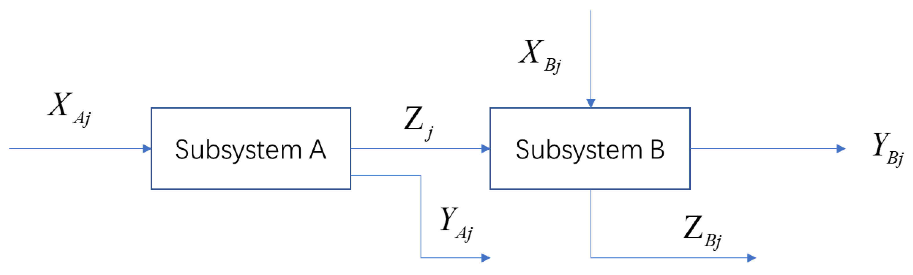
In the production context, it is assumed that there are n independent production systems, namely DMUs. A DMU can be divided into two subsystems, namely, the subsystem A and subsystem B. The two subsystems are connected in series to form a DMU, as shown in Figure 1, which is a classic network structure. For example, the factory would cause some pollutants while making products, and these pollutants must be dealt with before discharging. In the A subsystem of the j-th DMU, the input vector is $x_{Aj}$, the expected output vector is $y_{Aj}$, and the undesirable output vector is $z_{Aj}$. Among them, the expected output exits from the production system, and the undesirable output enters the B subsystem as the intermediate input. Additional inputs $x_{Bj}$ are needed in the B subsystem, which is denoted as the final output including expected output $y_{Bj}$ and undesirable output $z_{Bj}$. The notations used across the paper are defined in

Table A1. The vector notations used in Section 2.

Vectors	Meaning
$x_{Aj}$	Input vector of subsystem A
$y_{Aj}$	Desirable output vector of subsystem B
$z_{Aj}$	Undesirable output vector of subsystem B
$x_{Bj}$	Input vector of subsystem B
$y_{\mathrm{B}j}$	Desirable output vector of subsystem B
$z_{Bj}$	Undesirable output vector of subsystem B
${\mu }_A^T,v_A^T,{\omega }_A^T$	Weight vector for subsystem A before C-C transformation
${\overline{\mu }}_A^T,{\overline{v}}_A^T,{\overline{\omega }}_A^T$	Weight vector for subsystem A after C-C transformation
${\mu }_B^T,{\omega }_B^T,v_B^T$	Weight vector for subsystem B before transformation
${\overline{\mu }}_B^T,{\overline{v}}_B^T,{\overline{\omega }}_B^T$	Weight vector for subsystem B after C-C transformation
${\overline{\overline{\mu }}}_B^T,{\overline{\overline{v}}}_B^T,{\overline{\overline{\omega }}}_B^T,{\overline{v}}_A^T$	Weight vector for subsystem B after ratio transformation
$e_k^s$	System efficiency

(Appendix A).

This involves the issue of treatment of undesirable outputs. Here, we use the linear data transformation function method [7] proposed by Seiford to convert the undesirable output into desired output and satisfy the nature of the more, the better. That is

$${\overline{\mathrm{z}}}_j=P-z_j,$$

(1)

where P here is a sufficiently large positive number so that all undesired outputs are positive after the transformation.

2.1. The Two-Stage DEA Based on the Cooperative Game

In a cooperative game, the two subsystems should be equal, and they should cooperate with each other to achieve the optimal efficiency of the whole DMU. These two subsystems are connected by intermediate outputs, and only intermediate outputs can reflect the relationship between the two subsystems when they have the same weight.

In the cooperative game, the two-stage DEA model [26] is given as

$$\begin{array}{cc}\max & \frac{1}{2}\left[\frac{{\mu }_A^T{y}_{Ak}+v_A^T{\overline{z}}_{Ak}}{{\omega }_A^T{x}_{Ak}}+\frac{{\mu }_B^T{y}_{Bk}+v_B^T{\overline{z}}_{Bk}}{{\omega }_B^T{x}_{Bk}+v_A^T{\overline{z}}_{Ak}}\right]\\ s.t.& \begin{array}{l}\frac{{\mu }_A^T{y}_{Aj}+v_A^T{\overline{z}}_{Aj}}{{\omega }_A^T{x}_{Aj}}\le 1, j=1,2,\cdots ,n,\\ \frac{{\mu }_B^T{y}_{Bj}+v_B^T{\overline{z}}_{Bj}}{{\omega }_B^T{x}_{Bj}+v_A^T{\overline{z}}_{Aj}}\le 1, j=1,2,\cdots ,n,\\ {\mu }_A,{\mu }_B,v_A,v_B,{\omega }_A,{\omega }_B\ge 0.\end{array}\end{array}$$

(2)

Here, k indicates that the k-th DMU is evaluated. The undesirable output is treated by a linear data transformation function method. The system efficiency here is a convex combination of the efficiency scores of the two subsystems. Since the status of the two subsystems is equal, the weight of each subsystem is 0.5. The above fractional programming can be transformed into linear programming by means of Charnes–Cooper transform [27].

$$\begin{array}{cc}\max & \frac{1}{2}(U_A{y}_{Ak}+U_B{y}_{Bk}+V_A{\overline{z}}_{Ak}+V_B{\overline{z}}_{Bk})\\ s.t.& \begin{array}{l}{W}_A{x}_{Ak}=l\\ W_B{x}_{Bk}+V_A{\overline{z}}_{Ak}=l’\\ U_A{y}_{Aj}+V_A{\overline{z}}_{Aj}-W_A{x}_{Aj}\le 0, j=1,2,\cdots ,n,\\ U_B{y}_{Bj}+V_B{\overline{z}}_{Bj}-W_B{x}_{Bj}-{V^{\prime }}_A{\overline{z}}_{Aj}\le 0, j=1,2,\cdots ,n.\\ {V^{\prime }}_A=l{V}_A\\ U_A,U_B,V_A,V_B,W_A,W_B,{V^{\prime }}_A\ge 0\end{array}\end{array}$$

(3)

The nonlinear programming is transformed into linear programming with parameters. If the weight vectors here are all one-dimensional, that is to say, only one of the intermediate expected outputs, the fourth constraints can be removed directly, and there is no effect on the solution of the linear programming. If it is not one-dimensional, an interval between an upper bound for the parameter (l, l’) and zero can be obtained, and the parameters vary in the interval to get the maximum value of the objective function. Although the efficiency of the entire system can be uniquely determined, the efficiency of each subsystem is not necessarily unique.

2.2. The Two-Stage DEA Based on the Non-Cooperative Game

In the non-cooperative game stage, the two subsystems are unequal. Here, we assume that subsystem A is in a leadership position and subsystem B is in a subordinate position. The A subsystem first determines its own optimal weight. The efficiency evaluation model of A subsystem is [28]:

$$\begin{array}{cc}\max & \frac{{\mu }_A^T{Y}_{Ak}+v_A^T{\overline{z}}_{Ak}}{{\omega }_A^T{X}_{Ak}}\\ s.t.& \begin{array}{l}\frac{{\mu }_A^T{Y}_{Aj}+v_A^T{\overline{z}}_{Aj}}{{\omega }_A^T{X}_{Aj}}\le 1,j=1,2,\cdots ,n\\ {\mu }_A^T,v_A^T,{\omega }_A^T\ge 0.\end{array}\end{array}$$

(4)

Through the Charnes–Cooper transform, model (4) can be transformed into a linear programming problem:

$$\begin{array}{cc}\max & {\overline{\mu }}_A^T{Y}_{Ak}+{\overline{v}}_A^T{\overline{z}}_{Ak}\\ s.t.& \begin{array}{l}{\overline{\mu }}_A^T{Y}_{Aj}+{\overline{v}}_A^T{\overline{z}}_{Aj}-{\overline{\omega }}_A^T{X}_{Aj}\le 0,j=1,2,\cdots ,n,\\ {\overline{\omega }}_A^T{X}_{Ak}=1\\ {\overline{\mu }}_A^T,{\overline{v}}_A^T,{\overline{\omega }}_A^T\ge 0.\end{array}\end{array}$$

(5)

Since the B subsystem is in a subordinate position, it decides the best weight after the A subsystem determines the most favorable weight for itself. The intermediate output is connected to two subsystems, so when the B subsystem determines the weights of the intermediate outputs, he has to refer to its weight setting in the A subsystem. Thus, in different subsystems, the weight setting needs to be satisfied with ${\nu }_B^T=Q{v}_A^T$ ($Q\ge 0$). The efficiency of the B subsystem is [16]:

$$\begin{array}{cc}\max & \frac{{\mu }_B^T{Y}_{Bk}+v_B^T{\overline{z}}_{Bk}}{{\omega }_B^T{X}_{Bk}+Q{v}_A^T{\overline{z}}_{Ak}}\\ s.t.& \begin{array}{l}\frac{{\mu }_B^T{Y}_{Bj}+v_B^T{\overline{z}}_{Bj}}{{\omega }_B^T{X}_{Bj}+Q{v}_A^T{\overline{z}}_{Aj}}\le 1,j=1,2,\cdots ,n\\ {\mu }_A^T{Y}_{Ak}+v_A^T{\overline{z}}_{Ak}=e_k^{A*}\\ {\mu }_A^T{Y}_{Aj}+v_A^T{\overline{z}}_{Aj}-{\omega }_A^T{X}_{Aj}\le 0,j=1,2,\cdots ,n\\ {\omega }_A^T{X}_{Ak}=1\\ {\mu }_A^T,{\omega }_A^T,v_A^T,{\mu }_B^T,{\omega }_B^T,v_B^T\ge 0.\end{array}\end{array}$$

(6)

The model (6) is transformed, and the following problem can be obtained

$$\begin{array}{cc}\max & \frac{\frac{1}{Q}{\mu }_B^T{Y}_{Bk}+\frac{1}{Q}{v}_B^T{\overline{z}}_{Bk}}{\frac{1}{Q}{\omega }_B^T{X}_{Bk}+v_A^T{\overline{z}}_{Ak}}\\ s.t.& \begin{array}{l}\frac{\frac{1}{Q}{\mu }_B^T{Y}_{Bj}+\frac{1}{Q}{v}_B^T{\overline{z}}_{Bj}}{\frac{1}{Q}{\omega }_B^T{X}_{Bj}+v_A^T{\overline{z}}_{Aj}}\le 1,j=1,2,\cdots ,n,\\ {\mu }_A^T{Y}_{Ak}+v_A^T{\overline{z}}_{Ak}=e_k^{A*}\\ {\mu }_A^T{Y}_{Aj}+v_A^T{\overline{z}}_{Aj}-{\omega }_A^T{X}_{Aj}\le 0,j=1,2,\cdots ,n\\ {\omega }_A^T{X}_{Ak}=1\\ {\mu }_A^T,{\omega }_A^T,v_A^T,{\mu }_B^T,{\omega }_B^T,v_B^T\ge 0.\end{array}\end{array}$$

(7)

Let ${\overline{\mu }}_B=\frac{1}{Q}{\mu }_B, {\overline{v}}_B=\frac{1}{Q}{v}_B, {\overline{\omega }}_B=\frac{1}{Q}{\omega }_B$; then, Equation (7) can be transformed into

$$\begin{array}{cc}\max & \frac{{\overline{\mu }}_B^T{Y}_{Bk}+{\overline{v}}_B^T{\overline{z}}_{Bk}}{{\overline{\omega }}_B^T{X}_{Bk}+v_A^T{\overline{z}}_{Ak}}\\ s.t.& \begin{array}{l}\frac{{\overline{\mu }}_B^T{Y}_{Bj}+{\overline{v}}_B^T{\overline{z}}_{Bj}}{{\overline{\omega }}_B^T{X}_{Bj}+v_A^T{\overline{z}}_{Aj}}\le 1,j=1,2,\cdots ,n,\\ {\mu }_A^T{Y}_{Ak}+v_A^T{\overline{z}}_{Ak}=e_k^{A*}\\ {\mu }_A^T{Y}_{Aj}+v_A^T{\overline{z}}_{Aj}-{\omega }_A^T{X}_{Aj}\le 0,j=1,2,\cdots ,n\\ {\omega }_A^T{X}_{Ak}=1\\ {\mu }_A^T,{\omega }_A^T,v_A^T,{\overline{\mu }}_B^T,{\overline{v}}_B^T,{\overline{\omega }}_B^T\ge 0.\end{array}\end{array}$$

(8)

Let $t=\frac{1}{{\overline{\omega }}_B^T{X}_{Bj}+v_A^T{\overline{z}}_{Aj}}$, ${\overline{\overline{\mu }}}_B={\overline{\mu }}_{B}t, {\overline{\overline{v}}}_B={\overline{v}}_{B}t, {\overline{\overline{\omega }}}_B={\overline{\omega }}_{B}t, {\overline{v}}_A=v_{A}t$; then, Equation (8) can be transformed into

$$\begin{array}{cc}\max & {\overline{\overline{\mu }}}_B^T{Y}_{Bk}+{\overline{\overline{v}}}_B^T{\overline{z}}_{Bk}\\ s.t.& \begin{array}{l}{\overline{\overline{\omega }}}_B{X}_{Bk}+{\overline{v}}_A^T{\overline{z}}_{Ak}=1\\ {\overline{\overline{\mu }}}_B^T{Y}_{Bj}+{\overline{\overline{v}}}_B^T{\overline{z}}_{Bj}-{\overline{\overline{\omega }}}_B^T{X}_{Bj}-{\overline{v}}_A^T{\overline{z}}_{Aj}\le 0,j=1,2,\cdots ,n\\ {\mu }_A^T{Y}_{Ak}+v_A^T{\overline{z}}_{Ak}=e_k^{A*}\\ {\mu }_A^T{Y}_{Aj}+v_A^T{\overline{z}}_{Aj}-{\omega }_A^T{X}_{Aj}\le 0,j=1,2,\cdots ,n\\ {\omega }_A^T{X}_{Ak}=1\\ {\mu }_A^T,{\omega }_A^T,v_A^T,{\overline{\overline{\mu }}}_B^T,{\overline{\overline{v}}}_B^T,{\overline{\overline{\omega }}}_B^T,{\overline{v}}_A^T\ge 0.\end{array}\end{array}$$

(9)

In this way, we can obtain the optimal efficiency of the two subsystems respectively. The efficiency of the whole system can also be expressed as the weighted average of the optimal efficiency of the two subsystems

$$e_k^s=\frac{1}{2}\frac{{\overline{\mu }}_A^T{Y}_{Ak}+{\overline{\nu }}_A^T{\overline{z}}_{Ak}}{{\overline{\omega }}_A^T{X}_{Ak}}+\frac{1}{2}\frac{{\overline{\overline{\mu }}}_B^T{Y}_{Bk}+{\overline{\overline{\nu }}}_B^T{\overline{z}}_{Bk}}{{\overline{\overline{\omega }}}_B^T{X}_{Bk}+{\overline{\nu }}_A^T{\overline{z}}_{Ak}}=\frac{1}{2}\frac{{\mu }_A^T{Y}_{Ak}+{\nu }_A^T{\overline{z}}_{Ak}}{{\omega }_A^T{X}_{Ak}}+\frac{1}{2}\frac{{\mu }_B^T{Y}_{Bk}+{\nu }_B^T{\overline{z}}_{Bk}}{{\omega }_B^T{X}_{Bk}+Q{\nu }_A^T{\overline{z}}_{Ak}}.$$

(10)

Accordingly, we can obtain the two-stage DEA model of non-cooperative game in which the B subsystem is in the leading position and the A subsystem is in the subordinate position. In the DEA model of non-cooperative games, because the efficiency of each subsystem is the optimal solution of each programming, they are unique, so the efficiency of the whole system is also unique. Accordingly, we can obtain the two-stage DEA model of non-cooperative game in which the B subsystem is in the leading position and the A subsystem is in the subordinate position.

These models can be used to analyze the DMUs with two subsystems after the relationship of the two subsystems is determined. If one assumes that the two subsystems are equally important, model (3) can be used. If one assumes the two subsystems are not equally important, models (5) and (9) can be employed. How to determine the relationship of the two subsystems objectively is the precondition. In the following section, we present the method to determine the relationship between the subsystems objectively, which combines models (3), (5), and (9) to form the three-step method for two-stage DEA.

3. Three-Step Method for Two-Stage DEA

Previously, subjective determination of the status of the two subsystems in the whole system was considered, and the corresponding two-phase DEA model through cooperative game or non-cooperative game was used to analyze the environmental efficiency [28,29]. However, it may be not in accordance with the real situation. In order to reduce the subjectivity, the computation can be used rather than subjective choice. According to the relationship, we can classify the DMUs into different groups. Then, the corresponding two-stage DEA of cooperative or non-cooperative game can be used. Based on this, we propose the three-step method to solve the two-stage DEA.

Step 1 is to determine the weights of the two subsystems in each DMU using the model (11) and to determine the importance of each subsystem relative to the total system performance, i.e., the status relationship between the two subsystems.

Here, we identify the relationship between the two subsystems in the production system by the SBM model Tone, which was proposed by [27]. The A subsystem has $I_1$ inputs, $R_1$ desired outputs, and $L_1$ intermediate undesirable outputs. The B subsystem has $I_2$ inputs, $R_2$ desired outputs, and $L_2$ undesirable outputs. First, we calculate the system efficiency of the k-th DMU.

$$\begin{array}{cc}{E}_k^s=\min & \frac{\{1-[({\displaystyle \sum _{i=1}^{I_1}\frac{s_i^{(1)-}}{x_{ik}^{(1)}})/I_1]\}+\{1-[({\displaystyle \sum _{i=1}^{I_2}\frac{s_i^{(2)-}}{x_{ik}^{(2)}}+{\displaystyle \sum _{l=1}^{L_1}\frac{t_l^{(2)-}}{{\overline{z}}_{lk}^{(1)}}})/(I_2+L_1)]\}}}}{\{1+[({\displaystyle \sum _{r=1}^{R_1}\frac{s_r^{(1)+}}{y_{rk}^{(1)}}}+{\displaystyle \sum _{l=1}^{L_1}\frac{t_l^{(1)+}}{{\overline{z}}_{lk}^{(1)}}})/(R_1+L_1)]\}+\{1+[({\displaystyle \sum _{r=1}^{R_2}\frac{s_r^{(2)+}}{y_{rk}^{(2)}}}+{\displaystyle \sum _{l=1}^{L_2}\frac{t_l^{(2)+}}{{\overline{z}}_{lk}^{(2)}})/(R_2+L_2)}\}}\\ s.t.& \begin{array}{l}{\displaystyle \sum _{j=1}^n{\lambda }_j^{(1)}{x}_{ij}^{(1)}=x_{ik}^{(1)}-s_i^{(1)-},i=1,2,\cdots ,I_1}\\ {\displaystyle \sum _{j=1}^n{\lambda }_j^{(1)}{y}_{rj}^{(1)}=y_{rk}^{(1)}+s_r^{(1)+},r=1,2,\cdots ,R_1}\\ {\displaystyle \sum _{j=1}^n{\lambda }_j^{(1)}{\overline{z}}_{lj}^{(1)}={\overline{z}}_{lk}^{(1)}+t_l^{(1)+},l=1,2,\cdots ,L_1}\\ {\displaystyle \sum _{j=1}^n{\lambda }_j^{(2)}{x}_{ij}^{(2)}=x_{ik}^{(2)}-s_i^{(2)-},i=1,2,\cdots ,I_2}\\ {\displaystyle \sum _{j=1}^n{\lambda }_j^{(2)}{\overline{z}}_{lj}^{(1)}={\overline{z}}_{lk}^{(1)}-t_l^{(2)-},l=1,2,\cdots ,L_1}\\ {\displaystyle \sum _{j=1}^n{\lambda }_j^{(2)}{y}_{rj}^{(2)}=y_{rk}^{(2)}+s_r^{(2)+}},r=1,2,\cdots ,R_2\\ {\displaystyle \sum _{j=1}^n{\lambda }_j^{(2)}{\overline{z}}_{lj}^{(2)}={\overline{z}}_{lk}^{(2)}+t_l^{(2)+}},l=1,2,\cdots ,L_2\end{array}\end{array}$$

(11)

The undesirable output here is still converted to desired output by the method of linear function transformation. $x_{ij}^{(1)}$, $y_{rj}^{(1)}$, and ${\overline{z}}_{lj}^{(1)}$ respectively represent the inputs of the A subsystem, the expected outputs, and the treated undesirable outputs, and $s_i^{(1)-}$, $s_r^{(1)+}$, and $t_l^{(1)+}$ represent the slack variables corresponding to them, respectively. $x_{ij}^{(2)}$, $y_{rj}^{(2)}$, and ${\overline{z}}_{lj}^{(2)}$ separately represent the inputs of the B subsystem, the expected outputs, and the processed undesirable outputs ${\overline{z}}_{lj}^{(1)}$ from the A subsystem as inputs enter into the B subsystem. Furthermore, $s_i^{(2)-}$, $s_r^{(2)+}$, $t_l^{(2)+}$ and $t_l^{(2)-}$ represent the relaxation variables corresponding to them, respectively. ${\lambda }_j^{(1)}$ and ${\lambda }_j^{(2)}$ respectively represent the strength coefficients of the two subsystems in the same DMU.

Unlike the previous two-stage SBM model, there is no weighting of the two subsystems in the target function. In fact, the weights at each stage are subjective. Here, the connection between the two subsystems is not considered.

Step 2 aims to classify the DMU. The two subsystems are equal in status, the A subsystem is in the leading position, and the B subsystem is in the leading position.

After model (11) gets the optimal solution through the solver, we can get the efficiency of each subsystem and the efficiency of the whole DMU, respectively. The efficiency of the DMU is the objective function in model (11). The efficiency of the A subsystem and the B subsystem can be expressed as follows (here, the superscript * means that the variable is the optimal solution of model (11), which are obtained through solving the programming):

$$E_k^{(1)}=\frac{1-[({\displaystyle \sum _{i=1}^{I_1}\frac{s_i^{(1)-*}}{x_{ik}^{(1)}})/I_1]}}{1+[({\displaystyle \sum _{r=1}^{R_1}\frac{s_r^{(1)+*}}{y_{rk}^{(1)}}}+{\displaystyle \sum _{l=1}^{L_1}\frac{t_l^{(1)+*}}{{\overline{z}}_{lk}^{(1)}}})/(R_1+L_1)]}$$

(12)

$$E_k^{(2)}=\frac{1-[({\displaystyle \sum _{i=1}^{I_2}\frac{s_i^{(2)-*}}{x_{ik}^{(2)}}+{\displaystyle \sum _{l=1}^{L_1}\frac{t_l^{(2)-*}}{{\overline{z}}_{lk}^{(1)}}})/(I_2+L_1)]}}{1+[({\displaystyle \sum _{r=1}^{R_2}\frac{s_r^{(2)+*}}{y_{rk}^{(2)}}}+{\displaystyle \sum _{l=1}^{L_2}\frac{t_l^{(2)+*}}{{\overline{z}}_{lk}^{(2)}})/(R_2+L_2)]}}.$$

(13)

Then, we can obtain two weights to compare the relative importance of the subsystem in DMU.

$$w^{(1)}=\frac{1+[({\displaystyle \sum _{r=1}^{R_1}\frac{s_r^{(1)+*}}{y_{rk}^{(1)}}}+{\displaystyle \sum _{l=1}^{L_1}\frac{t_l^{(1)+*}}{{\overline{z}}_{lk}^{(1)}}})/(R_1+L_1)]}{\{1+[({\displaystyle \sum _{r=1}^{R_1}\frac{s_r^{(1)+*}}{y_{rk}^{(1)}}}+{\displaystyle \sum _{l=1}^{L_1}\frac{t_l^{(1)+*}}{{\overline{z}}_{lk}^{(1)}}})/(R_1+L_1)]\}+\{1+[({\displaystyle \sum _{r=1}^{R_2}\frac{s_r^{(2)+*}}{y_{rk}^{(2)}}}+{\displaystyle \sum _{l=1}^{L_2}\frac{t_l^{(2)+*}}{{\overline{z}}_{lk}^{(2)}})/(R_2+L_2)}\}}$$

(14)

$$w^{(2)}=\frac{1+[({\displaystyle \sum _{r=1}^{R_2}\frac{s_r^{(2)+*}}{y_{rk}^{(2)}}}+{\displaystyle \sum _{l=1}^{L_2}\frac{t_l^{(2)+*}}{{\overline{z}}_{lk}^{(2)}})/(R_2+L_2)}}{\{1+[({\displaystyle \sum _{r=1}^{R_1}\frac{s_r^{(1)+*}}{y_{rk}^{(1)}}}+{\displaystyle \sum _{l=1}^{L_1}\frac{t_l^{(1)+*}}{{\overline{z}}_{lk}^{(1)}}})/(R_1+L_1)]\}+\{1+[({\displaystyle \sum _{r=1}^{R_2}\frac{s_r^{(2)+*}}{y_{rk}^{(2)}}}+{\displaystyle \sum _{l=1}^{L_2}\frac{t_l^{(2)+*}}{{\overline{z}}_{lk}^{(2)}})/(R_2+L_2)}\}}$$

(15)

The weights here represent the relative importance of each subsystem to the overall system performance. This weight is not as subjective as the weight in the previous two-stage SBM model, and the objective weight is obtained through calculating the total efficiency of the system, and it can reflect the essence of DEA. Moreover, the efficiency of the total system can be decomposed into the weighted average of the efficiencies of two subsystems, ${\displaystyle \sum _{i=1}^2{\omega }^{(i)}{E}_k^{(i)}=}{E}_k^s$.

With this weight information, we can determine the importance of the two subsystems to the overall system. If the weight of the A subsystem is higher, it shows that the A subsystem is more important to the overall system, and the A subsystem should be placed first in order to be more conducive to the development of the overall system. Otherwise, the B subsystem should be placed first. If the weights of the two subsystems are equal, it shows that the A subsystem and the B subsystem are equally important to the overall system, and they are in an equal position. Depending on the weights, we can categorize DMUs into different groups according to the relation between its subsystems. Generally, they can be divided into three groups: namely, a group of two subsystems in an equal position, a group of A subsystems in a leading position, and a group of B subsystems in the leading position.

Step 3 The efficiency of each subsystem and the efficiency of the system are analyzed respectively by using the two-stage DEA of cooperative game or the two-stage DEA of the non-cooperative game in the three groups of DMUs. Rather than ad hoc analysis to determine the relationship between two subsystems according to the national policy, efficiency analysis with the three-step method can better reflect the essence of DEA, but it also reduces the subjectivity of decision-makers, and efficiency is more reasonable.

4. Numerical Example: The Environmental Efficiency Analysis in China

This section uses the above method to analyze the efficiency of the water environment of the industrial production system in 31 provinces in China. The industrial production system in each region is shown in Figure 2. Each region can be regarded as a DMU. Here, subsystem A is an economic development subsystem, subsystem B is an environmental protection subsystem, and B deals with the pollutants produced by A in industrial production and gets the final pollutants. Any industry would cause some inevitable pollution during production and try their best to deal with the pollution so that it would reduce the impacts on the environment. The inputs of the subsystem A include labor and fixed capital investment, which are the main inputs in industry, and A’s output includes expected output (gross industrial product) and undesirable output (industrial wastewater). The inputs of subsystem B include the investment and operating costs of industrial wastewater treatment facilities, and the output of subsystem B is final industrial wastewater discharge. We integrate the facilities inputs of subsystem B as a box in Figure 2. Here, intermediate industrial wastewater discharge and eventual industrial wastewater discharge are undesirable outputs, and they need to be dealt with by the linear data transfer function method. Here, the data mainly come from the “China Statistical Yearbook 2012” and “China Environmental Statistics Yearbook 2012”, as shown in

Table 1. Characteristics of all regional industry system’s inputs and outputs.

Subsystem	Notations	Indicators	Max	Min	Mean	Std. Dev
The economic development subsystem	$x_{Aj}$	Fixed investment (100 million RMB)	41,481.97	206.44	12,454.41	10,328.27
		Labor (10,000 people)	1451.14	1.63	295.72	330.90
	$y_{Aj}$	Industrial GDP (100 million RMB)	107,680.7	74.85	27,234.48	28,133.51
	$z_{Aj}$	Industrial wastewater (10,000 ton)	933,519	498	187,274.55	189,954.63
The environmental protection subsystem	$x_{Bj}$	Operation cost for handling the industrial waste water (10,000 RMB)	295,540	660	50,892	56,744.50
		Investment facilities for the industrial waste water (10,000 RMB)	8,111,854	232	1,434,314.70	506,528.03
	$z_{Bj}$	Discharge of industrial waste water (10,000 ton)	246,298	363	74,475.61	64,639.36

.

According to the three steps of solving the two-stage DEA, model (11) is used to obtain the optimal weights (14), (15) of the economic development subsystem and the environmental protection subsystem in each region; that is,

Table 2. The weights of the production subsystem and environment protection subsystem in each region.

Regions	The Weight of the Economic Development Subsystem	The Weight of the Environmental Protection Subsystem
Group B
Inner Mongolia	0.50	0.50
Fujian	0.50	0.50
Jiangxi	0.50	0.50
Hunan	0.50	0.50
Tibet	0.50	0.50
Hainan	0.50	0.50
Tianjin	0.50	0.50
Group A
Qinghai	0.75	0.25
Chongqing	0.76	0.24
Shandong	0.80	0.20
Anhui	0.81	0.19
Ningxia	0.82	0.18
Guangxi	0.85	0.15
Shanghai	0.86	0.14
Jiangsu	0.86	0.14
Beijing	0.88	0.12
Zhejiang	0.88	0.12
Guizhou	0.88	0.12
Gansu	0.88	0.12
Henan	0.89	0.11
Xinjiang	0.89	0.11
Jilin	0.90	0.10
Yunnan	0.91	0.09
Guangdong	0.92	0.08
Liaoning	0.93	0.07
Heilongjiang	0.94	0.06
Shaanxi	0.94	0.06
Sichuan	0.95	0.05
Shanxi	0.96	0.04
Hubei	0.96	0.04
Hebei	0.99	0.01

. We have to state that we only need to compare the weights of the two subsystems in one region, which indicate that the region emphasizes the economic development subsystem or the environmental protection subsystem. As for different regions, there is no meaning to compare their weights with each other.

Based on the weights of each subsystem in Table 2, we can analyze the status relationship between the two subsystems in each region. It is easy to see that for most areas, the economic development subsystem is more important to the development of the overall system. For a small number of areas, the economic development subsystem and the environmental protection subsystem are equally important to the development of the overall system. There are no regions that regard the environmental protection subsystem as more important than the economic development subsystem. The 12th Five-Year plan (2011–2015) from the Chinese government explicitly pointed out that the construction of a resource-saving and environment-friendly society could play a key role in accelerating the transformation of economic development of the important points in some areas. For example, Tianjin and Inner Mongolia have been aware of the seriousness of environmental problems and began to change the mode of development, making economic development and environmental protection simultaneously smooth to walk the road of sustainable development. However, most areas still give priority to economic development, and our government should be aware of this and formulate relevant policies to transform the mode of economic development in these regions. If we blindly think of two subsystems in all regions as equal status, the system efficiency of the two-stage DEA will adopt cooperative game, which is not proper for regions that prioritize the economic development system. Here, we use the above method to divide all the regions into two groups. The regions in which the economic development subsystem is prioritized are classified as Group A, and the regions in which the economic development subsystems and environmental protection subsystems are equally important are classified as Group B. Using the two-stage DEA model of cooperative game (model 3) for Group B and non-cooperative game (models 5 and 9) for Group A respectively, the efficiency of each subsystem and the whole DMU are analyzed and shown in

Table 3. The efficiencies of the subsystems and the whole region.

Regions	Efficiency of the Economic Development Subsystem	Efficiency of the Pollutant Disposal Subsystem	Efficiency of the Whole Region	Efficiency of the Whole System under Cooperation (Within-Group)	Efficiency of the Whole System under Cooperation (Global)
	(1)	(2)	(3)	(4)	(5)
Group B
Fujian	1	0.928	0.964	0.964	0.758
Tianjin	1	0.994	0.997	0.997	0.919
Inner Mongolia	1	1	1	1	0.936
Jiangxi	1	1	1	1	0.882
Hunan	1	1	1	1	0.831
Tibet	1	1	1	1	1
Hainan	1	1	1	1	0.974
Group A
Shanxi	0.647	0.743	0.695	0.695	0.674
Jiangsu	1	0.421	0.710	0.710	0.594
Shandong	1	0.419	0.710	0.710	0.647
Sichuan	0.800	0.635	0.717	0.717	0.694
Zhejiang	1	0.554	0.777	0.777	0.664
Heilongjiang	0.720	0.878	0.799	0.799	0.728
Shaanxi	0.752	0.853	0.802	0.803	0.737
Guangdong	1	0.606	0.803	0.803	0.671
Yunnan	0.767	0.902	0.834	0.834	0.738
Hubei	0.830	0.841	0.836	0.836	0.733
Henan	0.972	0.741	0.856	0.856	0.746
Liaoning	0.952	0.784	0.868	0.868	0.807
Guizhou	0.791	0.894	0.888	0.895	0.785
Gansu	0.872	0.96	0.916	0.916	0.831
Xinjiang	0.914	0.923	0.919	0.919	0.831
Anhui	0.982	0.889	0.936	0.935	0.866
Chongqing	1	0.905	0.953	0.952	0.874
Jilin	0.980	0.927	0.954	0.954	0.864
Guangxi	0.940	0.97	0.955	0.955	0.847
Hebei	0.947	1	0.973	0.973	0.954
Ningxia	1	0.956	0.978	0.978	0.764
Beijing	1	1	1	0.999	0.912
Shanghai	1	1	1	1	0.907
Qinghai	1	1	1	1	0.868
Mean	0.931	0.862	0.898

Note: The last two columns do not contain the average efficiency of the system when the cooperative status is given. While quantitative figures could be obtained, they would not make economic sense.

. The R language is used to carry out the corresponding computation.

In Table 3, regions in Group B regard the economic development and environmental protection subsystems as having the same importance, and the rest of the regions pay more attention to the economic development subsystem. Overall, the region efficiency of each area in China is still relatively high, and the economic development subsystem efficiency is higher than that of the environmental protection system in most parts of China. This is consistent with more regional important economic development subsystems in Table 2. We can see that for almost all the regions that regard the economic development subsystem and environmental protection subsystem as equally important, their system efficiencies are very high. Other than the system efficiency of Fujian (0.964) and Tianjin (0.997), the rest all achieved unity. For the areas that prioritize the economic development, such as Heilongjiang, Guizhou, Yunnan, Gansu, and other regions, although they pay more attention to the efficiency of economic development, the efficiency of the economic development subsystem is not necessarily better than that of the pollutant processing subsystem. These areas are economically underdeveloped areas; even if they give priority to the development of the economy, their pollutant processing subsystem efficiency is still high. There are some areas in the group whose overall system efficiency is not high. The main reason is that the efficiency of the environmental protection system is not high due to economic development, although the efficiency of their economic development subsystem is pretty high, such as Shandong, Henan, and other regions. These are all big economic provinces, but they do not pay much attention to the environmental problems in developing the economy, which leads to the reduction of the efficiency of the environmental protection subsystem; thus, the overall system efficiency is not high.

In the last two columns of Table 3, the efficiency of each region is obtained from the cooperative two-stage DEA model, which subjectively considers that the economic development subsystem and the pollutant treatment subsystem are equal. For the sake of comparison, we give the efficiency of two-stage DEA models using cooperative game. Column 4 calculates the system efficiency of each region within the two groups (A and B) under the two-stage DEA of cooperative game. Since they have the same production possibility set, we can compare the system efficiency obtained by this method with that obtained by two-stage DEA of cooperative game under grouping. Column 5 of Table 3 reports the system efficiency of each region under the two-stage DEA of cooperative game and a global reference set, including all the provinces. By comparing the last two columns in Table 3, we can see that the system efficiency in Column 5 is lower than that reported in Column 4. This is due to the change of the production possibility set. For example, the efficiencies of Guizhou are 0.895 and 0.785 within group and globally, respectively.

These results confirm that the provinces that give equal importance to the economic and environmental production processes (i.e., Group B) are more advanced than those where the economic production process is more important (i.e., Group A). However, the efficiency of certain provinces in Group B also declined due to the expansion of the reference set. For those regions whose economic development is more important, comparing the feasible regions of models (3) and (9), we can find that the system efficiency of cooperative game is not smaller than that of non-cooperative game. However, for these regions of China, such as Guangdong, the system efficiency of cooperative game is the same as that of non-cooperative game. It shows that even if the economic development is given priority, the system efficiency is also improved. In other words, these regions pay more attention to economic development, yet they are also on the road of sustainable development.

Finally, Beijing and Shanghai are China’s political and economic centers, and their regional government departments pay more attention to environmental protection, and industrial enterprises also attach great importance to environmental issues, during the development of the economy. Therefore, the efficiencies of the two regions are very high on the whole. As for Jiangxi, Hainan, Tibet, and Qinghai, these areas do not take industry as the main growth point of economy; therefore, there are no obvious pollution problems. Under the strategy of Western development, Tibet and Qinghai have strengthened their own technical and management levels and made rational investment in resources, so the efficiency of economic development in these areas is relatively high. The low efficiency areas are mainly Jiangsu, Zhejiang, and Shandong. The local private industry is relatively developed, but it is at the sacrifice of the environmental pollutions. Although the efficiencies of the economic development subsystem are very high, the efficiencies of the environmental protection subsystem are quite low, which means that the overall efficiencies of these regions are very low.

5. Conclusions

This paper presents a three-step method for solving two-stage DEA efficiency analysis. Through this method, the decision-maker does not determine the status relationship between the two subsystems subjectively according to the policy and other factors but rather determines the status relationship between the subsystems according to the optimal weights. According to the status relationship among subsystems, the region is divided into groups, and the two-stage DEA model of cooperative game or non-cooperative game is used to analyze the efficiency. This method reduces the subjectivity of decision making and helps choose the most appropriate model (two-stage DEA with cooperative game or non-cooperative game) for the DMUs with two stages, which is conducive to finding the source of low efficiency compared to the previous methods.

Finally, this paper verifies the rationality and validity of the method by analyzing the water environment efficiency of 31 industrial systems in China. The results suggest that the economic production process is more efficient if compared to the pollution generation approach as indicated by the mean efficiency scores. Accordingly, most of the provinces attach higher importance to the economic production process using the objective data-driven DEA weighting proposed in this paper. This indicates that the further promotion of the renewable energy and cleaner production practices should be furthered in most of the provinces of China. However, the results of the cooperative analysis (where efficiency is calculated assuming that the economic and environmental systems are equally important) show the same ranking of the provinces. Therefore, one may assume that pursuing economic development may also benefit the sustainable development as well in China’s provinces.

In this paper, we only focus on the DMU with the two subsystems that are connected in series, which is not very general. In the future research, one may focus on DMUs with more complex network structure to obtain the rational efficiency analysis methods. One can further analyze the links of the proposed model with such models as the by-production model encompassing the two subfrontiers. Further studies are needed to explore the dynamics in the Chinese economy over the more recent time period.