1. Introduction
Recently, environmental and economic concerns have further stimulated the efficient use of energy resources. From a generation standpoint, improvements in efficiency are attained mainly by three actions: (1) development of new technologies; (2) upgrade and retrofit; (3) better management of resources. Technological developments include, but are not limited to, large-scale energy storage [
1], and alternative energy sources such as hydrogen. Although essential, such developments are resource and time consuming. Upgrading and retrofitting existing power plants is a more immediate action that is especially appealing in countries with old power plants [
2]. The third option involves the planning and operation phases of power systems. While the planning phase considers time horizons of years to determine the construction and decommissioning of power plants and transmission lines, the operation phase is focused on the short term and is better represented by the day-ahead scheduling problem known as unit commitment (UC) [
3]. In the following, we discuss how the formulation and solution of the UC can affect the overall efficiency of a power system.
Despite being well studied and documented, the UC is still an open problem. In its most complete form, UC is a large-scale, uncertain, mixed-integer non-linear problem with, conservatively, millions of variables and constraints. This complete formulation is challenging because it is rarely possible to solve such a problem in a timely manner and, were it possible, it is not clear how energy prices could be derived from its solution (see [
4] for discussions on pricing in markets with nonconvexities). Thus, system operators often use simplified formulations of the UC to feed their decision-making processes. The simplifications include linearization of non-linear functions (such as power flows and power production), neglecting any explicit representation of uncertainty, and aggregation of smaller generating units. The linearization transforms the then mixed-integer non-linear problem into a mixed-integer linear problem, whereas removing uncertainty renders the problem deterministic. These two simplifications are important, not only for yielding a problem that is more easily solved, but also to arrive at a formulation that adheres to current practices of energy pricing. With unit aggregation [
5,
6] (sometimes also called unit clustering), identical units connected to the same bus are aggregated into a single unit. Thus, unit aggregation is a more subtle simplification: although it generally does not change the nature of the problem, it can significantly reduce the number of integer decisions. Evidently, to one degree or another, any simplification carries a cost to the representation of the actual operation of the system. In this paper, we are particularly interested in the effects of the aggregation of hydro units in a large-scale hydrothermal power system, and in the benefits of explicitly considering the forbidden zones of hydro generation. The forbidden zones, sometimes also called areas, are intervals of generation that either cannot be reached by the hydro power plant (for instance, generations that are well below the minimum generation), or should be avoided due to concerns with vibration and cavitation. Note that the aggregation in our work is different from the reservoir aggregation of [
7]. Furthermore, an in-depth study on unit aggregation similar to what is used in our work can be found in [
8], where the authors investigate different strategies for clustering identical and non-identical units based on different criteria and analyse the resulting computing times and approximation errors. A thorough review on short-term modelling for hydro-dominated systems can be found in [
5], which also includes discussions on different aggregation strategies and unit-based modelling choices for hydro systems. Moreover, further details on the unit aggregation particular to the Brazilian system can be found in [
9].
The majority of the works tackling hydrothermal UC problems (HTUC) with consideration of forbidden zones focus on systems with few plants [
5]. The authors of [
10] address the unit commitment of a cascade comprised of two large hydro plants with a total number of 26 hydro generating units. In their work, the hydraulic coupling and irregular forbidden zones are modelled via a combination of segments of the non-linear functions’ domains and quadrangle and polynomial approximations for each segment. The resulting mixed-integer non-linear problem is solved by an off-the-shelf optimization solver and the results are compared against the more usual mixed-integer linear problem obtained through the linearization of the non-linear functions. Irregular forbidden zones are also the subject of [
11], but, different from [
10], the irregular forbidden zones, represented by a piecewise linear function, yield a mixed-integer linear programming problem. The test system of [
11] is composed of two hydro plants with a total of 10 generating units. In [
12], the self-scheduling problem with forbidden zones is tackled with Lagrangian relaxation. On the other hand, ref. [
13] proposes different linearization techniques for the hydropower production function of a single hydro plant with 50 generating units. In [
14], the authors propose a two-step methodology based on a piecewise linearization technique for solving the unit commitment problem of a multi-unit plant. The same 50-unit plant of [
13] is used in the assessments of the method in [
14]. The works [
10,
11,
12,
13,
14] all handle self-scheduling problems in which generation targets have already been set, for instance, by the system operator, the generating units must be scheduled and dispatched to satisfy them while optimizing an appropriate objective function. To the best of our knowledge, the only work addressing a large-scale centralized unit commitment problem with explicit representation of forbidden zones is [
15]. However, ref. [
15] is focused mainly on the development of the methodology used for solving the HTUC. The state-of-the-art for cost-based centralized dispatch of large-scale hydrothermal systems before [
9,
15], applied unit aggregation to the hydro generating units and subsequently neglected any integer decisions related to hydro generation. In contrast, ref. [
16] uses a similar plant-based aggregation to [
9], but tackles the problem via Lagrangian relaxation. Consequently, all forbidden zones were neglected.
Different from the studies found in the literature, we tackle a cost-based, centralized HTUC of a real, large-scale system. Moreover, in contrast to [
15], here, we focus on analysing the operational benefits of considering an explicit representation of forbidden zones in a large-scale system. Our analysis provides insights into the importance of forbidden-zone representation. Furthermore, due to the lack of studies with a real system, our work is the first, to the best of our knowledge, to quantify the differences between aggregation approaches with no consideration of forbidden zones, and the explicit consideration of forbidden zones.
This work is organized as follows. In
Section 2, we discuss the challenges arising from explicitly representing the forbidden zones of hydro plants. We then present the aggregated model in
Section 3, followed by the zone-aware model in
Section 4. In
Section 5, we present the test cases used in our evaluations and the computational setting. Then, in
Section 6, we show and discuss the results. The final remarks are given in
Section 7.
2. Challenges of Forbidden-Zone Representations
In hydro-dominated systems, unit aggregation is generally applied to reduce the number of hydro generating units. For instance, if a given hydro plant has five identical generating units all connected to the same bus, then an aggregation can reduce the number of units from five to one. Suffice to say that, for systems with a significant number of hydro plants, such aggregation provides a considerable reduction in problem size. Nonetheless, this aggregation can have an undesirable effect: the operation limits of the individual hydro generating units might not be satisfied in the aggregated unit. One such limit that is usually neglected is the minimum generation. Hydro turbines are built to operate at certain generation levels set by the designer in order to avoid cavitation and mechanical vibration [
17]. Thus, if the minimum generation is not taken into account during the UC, then a redispatch phase after the UC might be necessary to reallocate generation to within the limits of the generation units. In Brazil, this reallocation is performed heuristically based on the expertise of the system operator. Consequently, there is no guarantee, from a mathematical viewpoint, that the new operation point after reallocation is anywhere near optimality. To illustrate how aggregation works, take, for instance, the Brazilian hydro plant Salto Caxias, which has four identical Francis turbines all connected to the same bus and each rated at 310 MW. For a net head of 65.5 m, the minimum generation for each turbine is 235 MW. These limits are summarized in
Table 1.
Given the limits of
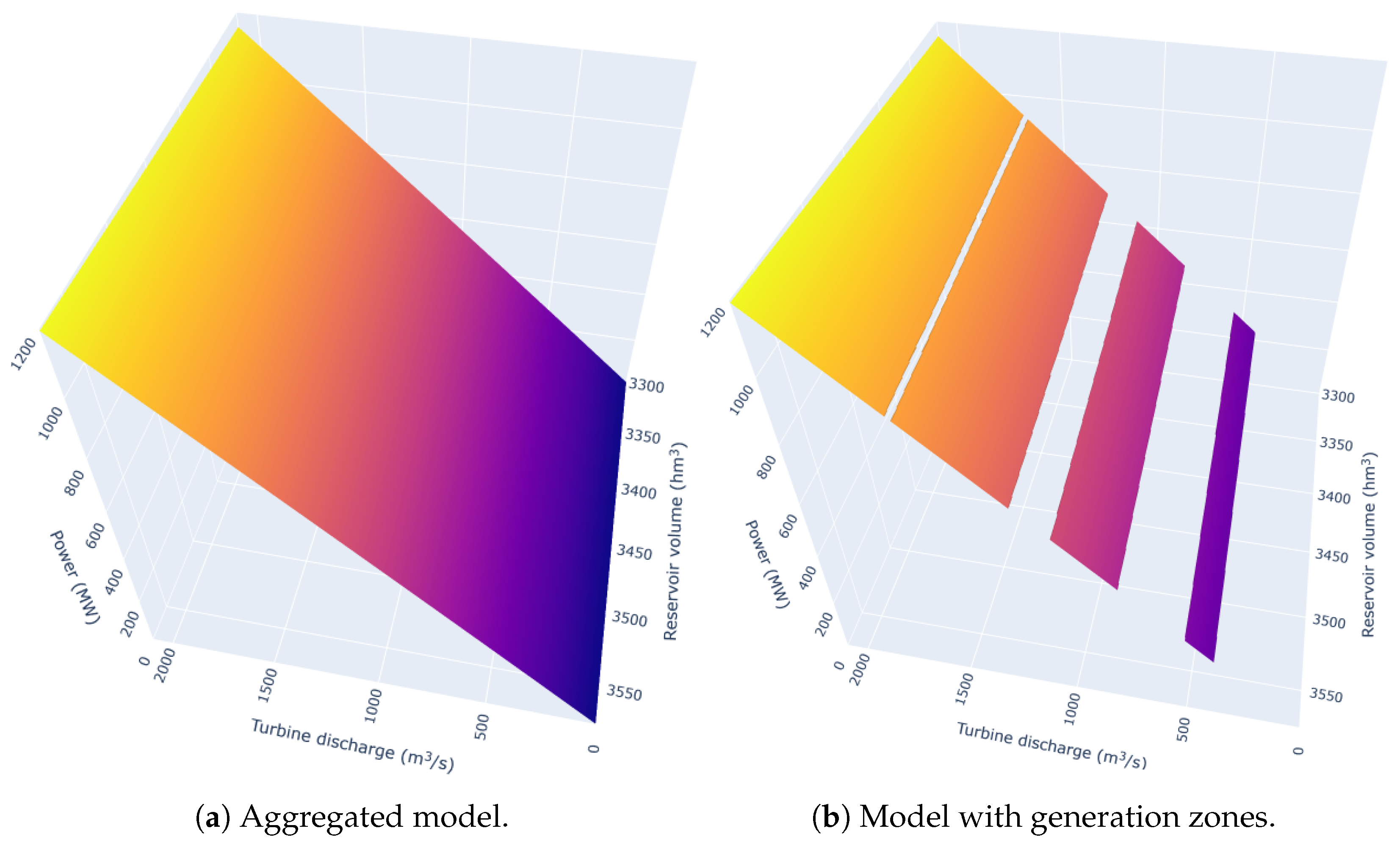
Table 1, and considering that there is no spillage, and the minimum generation of the units is not a function of the net head (the forbidden zones are regular), the total generation of Salto Caxias as a function of the total turbine discharge, i.e., the sum of the discharge of the four units, and the reservoir volume is shown in
Figure 1 for the aggregated representation of the plant and the representation with explicit operating zones.
Note that, under the aforementioned conditions, Salto Caxias has four forbidden zones: 0–235 MW, 310–470 MW, 620–705 MW, and 930–940 MW. The first and largest one is due to the minimum generation of a single unit: since all units have a minimum generation of 235 MW, in turn, the minimum generation of Salto Caxias itself is 235 MW. The second zone appears when one unit is operating but there is not enough power to turn on a second unit. In the event of operating in this second forbidden zone, then at least one unit would violate its minimum generation. Furthermore, it is possible to see from
Figure 1 that the generation limits also set limits on the turbine discharge. For the reservoir volume considered, the first operating zone has turbine discharges in the range 415–545 m
3/s. For Salto Caxias, unit aggregation can then aggregate its four units into a single large unit with minimum generation of 235 MW and maximum generation of 1240 MW. If, in addition to unit aggregation, no binary decision is associated with Salto Caxias, then its generation range is further relaxed to 0–1240 MW. Unit aggregation has further implications beyond the operation of the plant on which aggregation has been performed. Since hydro plants are generally connected to other plants downriver and upriver of them, unit aggregation of a plant can also affect the operation of downriver and upriver plants. To illustrate this point, take the six plants of the Iguaçu basin in
Figure 2.
Figure 2 shows part of the Iguaçu basin. In total, this basin encompasses nine reservoirs, the largest ones shown in the figure. Most hydro units installed along the Iguaçu river are Francis turbines. They generally have a relatively high minimum-generation level, which can lead to significant violations if an aggregation approach is used. Take, for example, the Salto Santiago plant, if at any given period one of its four units is to operate, then the turbine discharge of this plant must be such that the generation lies within 270 MW and 355 MW. In addition, consider, for the sake of argument, that the run-of-river plant Salto Osório has no reservoir regularization (its minimum and maximum reservoir volumes are the same), the only inflow to Salto Osório comes from Salto Santiago, and Salto Santiago cannot spill water (spillage is usually avoided since it essentially means a loss of opportunity for the plant spilling water). In this context, if Salto Osório is also scheduled to operate, then the turbine discharge from Salto Santiago must not only comply with the constraints of Salto Santiago itself, but also lie in one of the operating zones of Salto Osório. This simple example illustrates the challenges arising from considering an individual representation of generating units in a hydrothermal system. Evidently, such reasoning can be extended to all plant in the Iguaçu basin, and to the nearly 160 reservoirs of the Brazilian power system.
Figure 3 shows the minimum generation for each of the nearly 200 groups of identical units in the Brazilian system.
As can be seen in
Figure 3, the majority of the groups have a minimum generation below 50 MW. Thus, in an aggregated model,
Figure 3 shows that, for most power plants, the violations in the operation zones will be no greater than 50 MW. From the system’s viewpoint, while this threshold might seem negligible when seen individually, i.e., while a 50-MW violation might not warrant concern in a system where the mean load is above 50 GW, the occurrence of multiple violations can demand significant changes in the schedule given by the aggregated model.
To more quantitatively highlight the differences between the aggregated and individual hydro models, we again take Salto Caxias as an example. As previously mentioned, this plant has four identical units, and its installed capacity is 1240 MW. In the aggregated approach, Salto Caxias can generate at any level between 0 and its maximum. In (
1)–(
12), we show the aggregated model for a generic plant with a single group of identical units. For simplicity, we omit the indices for the hydro plant and its groups of units.
In (
1)–(
12), constants are given in boldface, while variables are in italic. In this model, constraints (
1), (
2), and (
3) limit from below and above the turbine discharge,
q, reservoir volume,
v, and the plant’s spillage,
s, respectively. In (
1), variable
u is used to select the operating zone
z of Salto Caxias, and
is the set of operating zones. In (
4), the inflow to the reservoir at a period
t is represented by variable
. In this simple example, this variable includes the incremental inflow and the discharge coming from upriver plants, and the function that determines its value is omitted for simplicity. Moreover, in (
4), constant
converts flows in m
/s to volume in hm
, i.e., it is 3.600 · 10
s. Constraints (
5)–(
9) form the piecewise linear model of the hydropower function: (
5) and (
6) limit, respectively, from above and below the generation potential,
, given by the forebay level (in this case, represented indirectly by the reservoir volume); similarly, (
7) and (
8) bound the generation loss,
, due to the tailrace level. The difference between
and
gives the plant’s generation,
, which is constrained in (
10) to lay between 0 and the plant’s installed capacity. In (
5)–(
9), constants
,
,
, and
, for
, are the coefficients of variables
q and
v in the piecewise model whose linear components are the indices
i in the respective sets
,
,
and
. Constraints (
11) are introduced to ensure that at most one variable
u assumes 1, while (
12) are the bounds on
u. Note that, since
u is continuous in this model, it is in fact possible to write an equivalent model without it. However, for a better understanding of the differences between the aggregated model and the zone model, we chose to keep variables
u. The following model, (
13) and (
14), is the equivalent forbidden-zone aware version of (
1)–(
12).
In (
13) and (
14), different from (
1)–(
12), the turbine discharge, and consequently the plant’s power output, depends on the binary variables
u. For this generic plant with a single group of identical units, there is one binary variable for each of its operating zones. In the particular case of Salto Caxias, there are four operating zones, i.e.,
, and the power limits of each zone are
,
,
,
MW, and
,
,
,
MW. The corresponding binary variables of the operating zones are
,
,
, and
for any given
t. Inequality (
11), now that
u is binary, guarantees that, at any given period, at most one operating zone can be chosen. Note that in (
13) and (
14) and (
1)–(
12), the model is the same, apart form the discontinuities in the permitted values for the turbine discharge and the generation in (
13) and (
14) that are the consequence of the now binary nature of
u. As one particular complicating factor, note that the turbine discharge chosen, and, consequently, the binary variable, must comply not only with its bounds, but also with the reservoir’s balance constraint, (
4). In terms of model size, explicitly representing the permitted operating zones of Salto Caxias introduces four binary variables, while the number of constraints remains the same. However, while in (
1)–(
12) these limits do not depend on any variable, in (
13) and (
14), the range of the turbine discharge and generation depend on the binary variables
u associated with the operating zones. The differences between (
1)–(
12) and (
13) and (
14) lead to discontinuities in the hydropower function shown in
Figure 1.
With the simple and generic example shown above, we now proceed to stating the HTUC with aggregated hydro generation used in this work.
3. Aggregated Hydrothermal Unit Commitment
We present in the following the optimization model used for representing the HTUC with the aggregated hydro model. For a better understanding, the model is separated into convenient parts. Firstly, we show the basics of the hydro model in (
15)–(
31).
In (
15)–(
31),
is the index of a hydro plant,
is a time period, and
is the index of a group of identical units at arbitrary plant
h. Furthermore, variable
u is used to identify the current zone in which the group of units is operating; set
contains the indices that identify the operating zones. In (
15)–(
31),
u is now subscripted with four indices: the hydro plant
h, the group of identical units
u, the operation zone
z, and the time period
t. Similarly, the set
of interested is specified with subscripts
h and
u. In the definitions that follow, we omit the variables’ units for brevity. In summary, all hydro flow variables are in m
/s, the volumes are in hm
, and the power generation is in
with 100 MW as basis. The coefficients and constants are assumed to have the appropriate units according to the aforementioned rules.
In (
15)–(
31), (
15) limits the total turbine discharge,
q, of each group of units. In this constraint, the upper bound on
q depends on variable
u. However, since in this aggregated model
u is continuous,
q can assume any value between 0 and the maximum turbine discharge. Seldom, reservoirs have other controllable means of discharging water to other reservoirs. One such means is here called a water bypass,
. Different from discharging water through the turbines or spilling, bypassing does not affect the power generation directly—only indirectly due to the reduction of the reservoir’s forebay level. The lower and upper bounds on water bypass are given in (
16). Note that, although only a handful of reservoirs dispose of this feature, (
16) is written for all reservoirs in the power system. This is done to avoid excessive notation. Evidently, reservoirs not disposing of a water bypass can simply have its upper limit,
, set to zero. Similar to a water bypass, some plants may have pumps installed along their reservoirs and, with them, downriver plants can send water to upriver plants (at the cost of actually consuming energy rather than generating it). The maximum rate of pumped water,
, is given in (
17). Again, note that, for those plants with no pumping mechanisms, the upper limit
can be set to zero. The more usual spillage,
s, has its limits given in (
18). Additionally, the reservoir volume,
v, is required to be at all times between its minimum,
, and maximum,
, as enforced by (
19).
The changes in the reservoir volume itself depend on the net balance between the total inflow to the reservoir and the total outflow. In (
15)–(
31), the inflow is represented by
a and defined in (
20) as a function of water discharges from turbines and spillages from upriver reservoirs, the term
, water bypass, and pumped water, and the constant incremental inflow,
. In (
20),
are sets of reservoirs capable of sending water to
h. For instance,
is the set of all plants upriver of
h whose turbine discharge and spillage reach
h after
d periods of time. Similar to
,
is the set of upriver plants to
h whose water bypass reaches
h. Lastly,
is the set of plants for which the pumped water arrives at
h. In (
20), the total inflow
a is represented in the same unit as the reservoir volume, thus, all rates are converted to volumes through the constant
. In contrast to (
20), (
21) gives the total outflow,
o, of each plant in each period. Finally, (
22) ensures that the mass balance in the reservoirs is satisfied at all times. In hydro systems, it is crucial to evaluate the trade-off between generating power now and saving water to generate power later. In this work, such evaluation is performed with a piecewise-linear cost-to-go function, (
23). In (
23),
is a set of indices defining the piecewise linear function that bounds from below the future cost
. This cost is given as a function of the reservoir volumes at the last period of the planning horizon,
.
An important modelling detail of any HTUC is the hydropower function. Here, we use the same hydropower-function model used in [
15], adapted to the context of explicit operation zones. As in [
15], (
24) and (
25) bounded from above and below, respectively, the potential power,
. On the other hand, (
26) and (
27) limit the power loss,
. Effectively, the hydro generation,
, is then the difference between the potential power and the power loss, as in (
28). Finally, the hydro generation of each group of units is bounded in (
29). Since model (
15)–(
31) is aggregated, the generation of each group of units can take any value between 0 and its maximum,
. Constraints (
30) and (
31) are included in the aggregated model to highlight the differences between this model and the zone model.
In addition to constraints (
15)–(
31), the operation of hydropower systems is further constrained by other uses of water. For instances, at some points, the river levels must be kept above a certain minimum to ensure navigability. Therefore, the outflow of power plants along said river are usually tightly controlled to satisfy the river’s minimum level. Likewise, environmental and agricultural concerns can also limit the operation of power plants. To reflect such limits, constraints (
33)–(
48) are introduced into the model. Note that, again, we choose to present the constraints as though they are presented in all power plants for the sake of conciseness. Evidently, those power plants which do not have such limits can have their respective bounds appropriately set to make their inequalities redundant.
Inequalities (33)–(39) bound the hydro variables to be within the respective time-dependent limits and . For example, reservoir volume for a given plant h and time t must be at least and not greater than . In addition to limiting the values, the rates of changes of the hydro variables are also limited in (40)–(48) by ramp constraints. Take, for instance, (43), these inequalities enforce that the change in outflow , for an arbitrary plant h and time t, from time to t must satisfy the maximum decrease in outflow for that plant and period, , and the maximum increase, . Generally, due to concerns with stability and security, sets of power plants may have their combined generation limited. In (48), set contains the indices representing such limits for period t. Hence, for a given t and one of its hydro generation limits , is the minimum generation and is the corresponding maximum for given groups of units of the plants in . In (48), not all groups of a plant in might participate in the constraints. Thus, indicates the groups of units of plant h participating in the generation constraints i.
With the hydro model defined as above, we now turn our attention to the thermal model. The first part of this model involves only the binary decisions associated with the thermal units, as shown in (
49)–(55).
The first constraint in (
49)–(55), (
49), determines the current phase of the thermal unit: off, in start-up trajectory, in shut-down trajectory, or in dispatch. In all phases but off, the status variable
x assumes 1. If the unit is in the start-up trajectory, then the sum on the start-up decisions,
, gives 1 and all variables in the equation other than
must assume 0. Similarly, in the shut-down trajectory, only the status variable and one of the shut-down decisions,
y, assume 1; if the unit is in the dispatch phase, then
k and
x assume 1. To guarantee that once a unit is brought on it remains at least one time period in the dispatch phase, constraints (50) are introduced. Constraints (50) and (52) are the usual minimum up- and down-time constraints. The logical constraints (53) dictate the relation between the status of the unit and the start-up and shut-down decisions. Since in this particular work start-ups and shut-downs are not economically penalized, constraints (54) are used to ensure that they do not occur at the same time. Finally, the binary nature of these decisions is given in (55). Now, the continuous part of the thermal model is given in (
56)–(60).
As previously stated, in this work, a thermal unit can be in one of four states. Equality (
56) defines the unit’s generation, in a per-unit basis,
according to the current state. The second term in (
56),
, gives the generation in the steps of the start-up trajectory; likewise,
defines the generation in the shut-down trajectory; while in the dispatch phase, the generation is simply equal to the generation in the dispatch phase itself,
. Whereas in the start-up and shut-down trajectory the unit must strictly follow a pre-defined set of generation steps, in the dispatch phase, its generation is more flexible. Nonetheless, it must still comply with the physical limits of the unit. Constraints (57) are the minimum and maximum generation in the dispatch phase, and constraints (58) and (59) are, respectively, the ramp-down and ramp-up constraints. Similar to the hydro plants, the combined generation of sets of thermal units can be further limited by the system operator. In (
56)–(60), constraints (60) give lower and upper bounds to the combined generation of the thermal units in set
, for a given constraint
of an arbitrary time
t.
The hydro and thermal models have been defined above. In the following, we show how the network constraints couple these models. In this work, we use a DC model, where the fluxes in the transmission lines is linearly dependent on the power injections at the buses.
The main objective of generation and transmission systems is to serve the demand for electrical energy. The equations (
61) establish that the power injections and withdrawals at each bus
must balance each other out. In (
61), the terms
and
are the total generations of thermal units and groups of hydro units connected to bus
b, respectively. In these terms, the sets
and
are, respectively, the thermal units connected to bus
b and the hydro plants connected to
b. Since all groups of hydro units at the same plant might not be connected to the same bus, set
gives the groups of units of plant
h connected to
b. The flow injections to bus
b are
and
. The positive term comprises all lines connected to
b whose positive-direction flow is, by convention, defined to inject power at
b—these lines comprise the set
. On the other hand, those lines whose, by convention, positive-direction flow withdrawals power from
b form the set
. In addition to the usual demand at each bus, hydro stations with pumps also demand power from the system. In (
61), set
contains the hydro plants whose pumps are connected to bus
b. The conversion from discharge through the pumps to power is performed with the constant
. Finally, the last terms in the left-hand side of (
61) are slack variables:
and
. Although shortage and excess of generation are not accepted in the normal operation of a power system, these variables are used in the mathematical model so that small violations in the power balances do not prevent quality solution from being chosen. The positive term,
, accounts for shortages of generation, while
covers surpluses. The non-negativity of both are enforced in (64). The right-hand side of (
61),
, is the constant power demand at each bus and time. For the DC model chosen, the flows in the transmission lines are written in terms of buses’ voltage angles,
. Constraints (62) gives such relations, where
is the impedance of line
l, and
and
are, respectively, the from and to buses of line
l. The flows are then set to be within the box constraints (63).
With all components defined above, the aggregated-hydro-model unit-commitment problem is defined in the following.
The objective function of (
65) is composed of three terms: the first one is the total cost of the thermal generation, the second is the cost of network violations, and the last one is the estimate of the future cost. Together, the cost of thermal generation and network violation form what we refer to in the rest of the text as the present cost. The objective function is minimized over the feasible region defined by the aggregated hydro model, (
15)–(31), the additional constraints on hydro variables, (
32)–(48), the integer model of thermal units, (
49)–(55), their continuous part, (
56)–(60), and, finally, the DC network constraints, (
61)–(64).
4. Forbidden-Zone-Aware Hydrothermal Unit Commitment
As previously stated, the model shown in the last section allows for the hydro generation to assume any non-negative value up to the plant’s maximum generation. Nonetheless, due to minimum generation requirements for the hydro units, the hydro generation curve is not continuous—as the example of
Figure 1 illustrates. In order to introduce into the HTUC of the previous section the discontinuities of the hydro generation, we need to resort to binary variables, as shown in the example of (
1)–(12) and (
13) and (14). Therefore, to accommodate the forbidden zones, model (
65) is further equipped with the integrality constraints shown in (
66).
As can be seen, the HTUC with aggregated hydro representation is, in fact, a relaxation of the commitment problem with explicit representation of the hydro zones. To see that, simply note that the only difference between the two models lies in the integrality of
u, which is missing in the aggregated model (
65). The fact that the aggregated model is a relaxation of the zone model guarantees that any differences in the optimal values of the two models are due to the integrality of
u which, in turn, is a consequence of the representation of the forbidden zones.
Additionally, note that the use of forbidden zones allows not only for a better representation of the limits on hydro generation, but could also be a means of improving the model of the hydropower function itself. In the aggregated model, the hydropower function is approximated through a single piecewise linear function for the entire range of the generation, from zero to the maximum, although some generation points might be forbidden. On the other hand, the inherently discontinuous nature of the generation in the forbidden-zone-aware model allows for the hydropower function to be approximated by a different model for each of the operating zones. Take again the example of
Figure 1, this plant has four operating zones. With additional (continuous) variables in (
66), the four operating zones of the plant in this example could be individually approximated by models of the hydropower function for each zone. Although a promising idea, to avoid potential disparities arising from different models of the hydropower function in the aggregated and the zone model, this paper focuses solely on the impacts of explicitly representing the operating zones of power plants in the HTUC.
Before presenting the computational experiments and the associated results, we first present the optimization model used to identify and quantify violations of the operating zones caused by the aggregated model (
65). To that end, we first note that there are several ways to perform this task: one could think of the violations on a basin basis, region basis, or plant basis. The first one could take into account the coupling of the reservoirs and the fact that violations in one hydro plant can likely affect the operation of reservoirs upstream and downstream of it. The second one could be based on the premises that power stations, hydro or otherwise, that are electrically close to each other are more likely to be affected by violations in operating zones. Naturally, the first two strategies for quantifying and analysing the violations of operating zones of hydro plants depend on the third one: if there is no violation for any of the hydro plants in the system, then the operation of the reservoirs in all basins and the operation of plants across the entire system will not be affected by violations. Thus, in this paper, we use a plant-based analysis for the violation of the operating zones in the aggregated model (
65). The model for this analysis for a arbitrary plant
h and arbitrary time period
t is shown in (
67).
In (
67), we simply take the generation of the groups of units of plant
h in time
t yielded by the aggregated model (
65),
, and check if such generation lies within one of the operating zones of plant
h by measuring the minimum Euclidean distance
d of
to the operating zones of
h. Evidently, if the optimal value of
d is 0, then
is, in fact, feasible in (
66). Otherwise, a positive optimal value of
d indicates that the feasible value of
closest to
is more than
. On the other hand, a negative optimal
d indicates that the closest operating zone to
is above
. Note that, although a simple model, (
67) enables us to identify violations generated by the aggregated model (
65) that ultimately need to be corrected by adjusting the operation of the plant violated itself, and, possibly, also of other reservoirs in the same cascade and of other power plants.
6. Results
We start our analysis by showing the bounds for each case and model in
Table 3. In this table, we give the best (min) and worst (max) upper bounds for each case over the five trials. Since the methodology in [
15] gives an essentially deterministic lower bound, this bound is unchanged over the trials of each case. As we mentioned in the statement of the models, the aggregated model is a relaxation of the zone model. Therefore, the optimal value of the zone model will be not less than the optimal value of the aggregated model. Since we are not able to solve the optimization models to optimality, we need to rely on the bounds of the optimization models. The difference between the lower bound of the zone model and the upper bound of the aggregated model give an underestimate on the difference between the optimal costs, whereas the difference between the upper bound of the zone model and the lower bound of the aggregated model gives an overestimate.
Take, for instance, Case 1, the best upper bound for the aggregated model for this case is $108,458,103.84 and the lower bound for this model is $108,366,249.0 . For the same case, the best upper bound for the zone model is $108,447,723.49 and the lower bound is $108,369,725.0 . Thus, for Case 1, the difference between the optimal costs of the aggregated and zone models lies in $[−88,378.84, 81,474.49] . However, since we know that the aggregated model is a relaxation of the zone model, then the underestimate on the difference between the optimal costs is, at least, 0. Then, the range of the difference for Case 1 is $[0, 81,474.49] . The worst case in terms of the overestimate of the increase in costs is Case 7, where the difference between the optimal costs can be as much as $86,982,200.36. A more practical measure of the differences in costs is the simple comparison of upper bounds. In this case, it is interesting to note that, for Cases 1 and 3, the upper bounds of the zone model are better than those of the aggregated model, whereas, for Case 8, the cost of the zone model’s solution is $34,242,315.15 greater than that of the aggregated model. Evidently, these are loose estimates of the differences between using the aggregated and the zone model in the decision-making process of the day-ahead operation. A more accurate analysis would require recomputing the costs of the aggregated model after redispatching the generating units due to (possible) violations of forbidden zones, and then comparing the costs after redispatch with the upper bounds given by the zone model. Unfortunately, such redispatch is commonly performed based on the experience of experts, and thus any attempt at reproducing them here would result in an unfair, and possibly biased, analysis.
Next, in
Table 4, we show the relative optimality gaps and the elapsed times for each case and model. Again, to account for the differences in the solutions obtained and the run times of each case over the five trials, we give the best (min) and worst (max) gaps and elapsed times of each case over the five trials. The worst gaps in
Table 4 indicate that all cases have been solved to a 0.1% optimality gap for both models in less than 30 min. Moreover, in the elapsed time’s column, we see that the computing times favor the aggregated model only slightly. In fact, the average run time of this model over all cases and trials is about 10 min, while that of the zone model reaches 10.5 min. Considering the magnitudes of the problems at hand, these computing times are well within the requirements for unit-commitment problems.
The first step of the multi-search Benders algorithm is to find an initial reference solution that is feasible in the original problem, although not necessarily a good solution in terms of costs. This step consists of three phases: (1) getting an estimate of the future cost; (2) solving a zero-objective continuous version of the original problem; (3) and finally getting binary solutions from the possibly fractional ones of phase (2). Phases (1) and (2) are essentially the same for the aggregated and the zone models, while phase (3) only differs due to the fact that, in the zone model, we need binary decisions for the hydro operation. Thus, it is not unreasonable to expect that the initial solutions of the aggregated and zone model can be rather close to each other, especially when we look at the thermal operation. After this first step to get the initial reference solution, the original problem is decomposed into multiple identical master problems and multiple identical sub problems. For both models, the sub problems are essentially the same in terms of model size: the aggregated model only has the additional continuous hydro variables in [0, 1], which account to roughly 15,000 variables, a relatively small number. Therefore, the running times of the sub problems for both models can be expected to be close. On the other hand, the master problems in the case of the zone model have an additional 15,000 binary variables, and this number, although relatively small, now becomes more significant because it relates to binary variables. However, our algorithm partitions the master problem’s variables into a set of free-to-change variables and a set of fixed variables. This dramatically reduces the computational complexity of the master problem because we are, in practice, getting rid of a substantial number of binary variables. Hence, the running times of the master problems of the zone model are greatly reduced due to this partitioning strategy. In conclusion, due to the similarity of the sub problems and the partitioning of the master problem, the overall running times of our algorithm for both models can be rather comparable, as seen in
Table 4.
To illustrate the violations in the operating zones in the aggregated model, we again use Salto Caxias as an example.
Figure 6 presents the generation of this plant in the aggregated model for each of the five trials of Case 4.
As it can be seen in
Figure 6, most of the violations in Salto Caxias happen during periods of low demand—this can be readily seen by analysing the demands in
Figure 4. Moreover, the majority of the violations are within the first forbidden zones, i.e., between 0 and the minimum generation of 235 MW. The example of
Figure 6 is also useful to demonstrate how the optimization model (
67) computes the violations. For instance, in the fifth half-hour, the generation of Salto Caxias is 117.4 MW in all trials. For this generation, the closest operating zone of Salto Caxias is 0—the distance to the minimum generation is 117.6 MW (
), while the distance to zero is 117.4 MW (
). Therefore, the violation for Salto Caxias in period 5 of Case 4 for all trials is 117.4 MW.
Figure 7 presents the violations of Salto Caxias’ operating zones for Case 4.
Using Trial 1 as an example, we can compute the average of the violations shown in
Figure 7 over the periods when they are strictly greater than 0. For Trial 1, this metric is 117.4 MW. The important thing to remember about a violation of this magnitude is that it requires significant changes in the operating point given by the aggregated model. This redispatch, in turn, is likely to be far from optimal if the day-ahead operation is not reoptimized (which is usually what happens since the redispatch is performed based on the experience of experts).
To gain a bigger picture of the violations over all cases for all plants, we can compute the total violations over all cases and trials, taking into consideration only violations greater than 10 MW—violations smaller than 10 MW are here considered to be more easily corrected. For a better understanding, note that each of the 10 cases has 48 periods, and each of the is run five times (the five trials). Thus, the total number of generation points to be analysed is
. For an arbitrary plant
h, assume that its violation in a case
c, with
, trial
i, with
, and time period
t is
, then the total violation is
. In addition to the total violation, we can also compute the occurrences of violations greater than 10 MW as
. Nonetheless, the aforementioned metrics are hard to understand due to their magnitudes, it is more interesting to see, first, the average of the violations over all cases and trials, defined as
, and the percentage of time periods in which the plant has its operating zones violated by more than 10 MW, i.e.,
.
Figure 8 shows the average violation and occurrences (given as percentages) of the 20 plants with most total violations over all cases and trials.
The first thing to note in
Figure 8 is the percentage of time that the plant Machadinho has violations, over 78%. Moreover, the average violation for this plant is 106 MW. The Machadinho plant has three identical Francis turbines with a generation range of [260, 380] MW. For the majority of time, the violation occurs in the first forbidden zone, i.e., in (0, 260) MW. The next plant in terms of frequency of violations is Itá, which for about 75% has violations that average 55 MW. In addition to the violations themselves, it is important to note that Machadinho is upstream from Itá, which adds to the difficulty of adjusting the generations of both plants. In fact, from the 20 plants shown in
Figure 8, four of them, Machadinho, Itá, Foz do Chapecó and Barra Grande, are in the Uruguai basin. Another basin which has a significant number of reservoirs in
Figure 8 is the Iguaçu, with three representatives: Salto Caxias, Salto Osório, and Segredo. Another plant whose violations warrants attention is Belo Monte. Although the frequency of violation for this plant is 9%, significantly less than the frequencies for the other plants in
Figure 8, its average violation is 163 MW, reaching a maximum of 218 MW. In contrast to the plants discussed here so far, Belo Monte has a great number of units, 18, all of them with a minimum generation of 450 MW. In addition, Belo Monte is a run-of-river plant built to exploit the high inflows in the wet period of Northern Brazil. Thus, when there is enough inflow, Belo Monte’s units operate near full capacity. However, in dry periods and/or periods of low demand, the high minimum generation of its units makes Belo Monte a likely candidate for violations.
Hitherto, we have focused on the violations in the hydro operating zones caused by the aggregated model. Now, we include in our analysis the zone model. First, we use the generation of Belo Monte in Trial 1 of Case 9 as an example—in fact, the dispatches for Belo Monte in all trials of Case 9 for both models are similar.
Figure 9 shows the plant’s generation over the 48 periods of the planning horizon. Note that, in the aggregated model, the generation violates all three forbidden zones. Moreover, Belo Monte’s generations in the two models are considerably different: while in the aggregated model, the total energy generation is 45,408 MWh, the total energy generation in the zone model is about 34,107 MWh. Furthermore, the peak generation in the aggregated model reaches 4668 MW, whereas in the zone model it is about 2927 MW.
In addition to the differences in the generation of individual hydro plants, the aggregated and zone models can also differ in the total generation.
Figure 10 illustrates this fact for the first trial of Case 1. In this figure, we see that the hydro generation in the zone model is considerably higher than that in the aggregated model. If we look at the examples previously shown of Salto Caxias and Belo Monte, the increase in generation in the zone model seems reasonable: since most violations occur in the first forbidden zone, the adjustment can be either to generate 0 (decrease), or generate at the minimum (increase).
Evidently, the increase in hydro generation presented in
Figure 10 reflects in a corresponding decrease in thermal generation, which is shown in
Figure 11.
The differences in thermal generation also reflect changes in the commitment of thermal units. To illustrate these differences, we again resort to Case 1 Trial 1. The total number of thermal units committed in each half-period of Case 1 Trial 1 is shown in
Figure 12. We care to note that the differences seen in this figure for the first trial are also seen in the other four trials. Moreover, with the exception of Cases 5 and 8, all cases show significant differences between the aggregated and zone model. (By significant difference, we mean that, for at least 12 h of the 24 h of the day-ahead operation, the difference in the number of committed units is at least 20.) As seen in
Figure 12, the difference in the number of committed thermal units can be as much as 70, which illustrates a significant difference in the operation of the system for a single day.
As we mentioned above, in Cases 5 and 8 the commitment of thermal units is similar for models aggregated and zones. We use Case 8 Trial 1 to illustrate this similarity in
Figure 13.
Although the commitment of thermal units is similar in this case, their total generation is still significantly distinct. In
Figure 14, we can see that the thermal generation in aggregated model is 879 MW higher than the generation in the zone model in the 40th half-hour.
The most apparent consequence in the changes in thermal generation shown in
Figure 11 are differences in the present costs of the system. To illustrate such changes, we show in
Figure 15 the average thermal generation costs for each case over the five trials. From this figure, it can be seen that, for most cases, there is a noticeable increase in thermal costs in the aggregated model, suggesting that the decrease in thermal generation, from the aggregated to the zone model, presented in
Figure 11 is also found in most of the other cases. Two cases that are exceptions to this trend are Cases 4 and 8, for which the costs in the zone model can be slightly higher than those in the aggregated model.
Another important metric in a hydro-dominated system is the stored energy left in the reservoirs at the end of the planning horizon. The more energy stored in the reservoirs, the less thermal generation will be required in the future—resulting in lower future generation costs. Here, we use the methodology presented in [
21] to compute the stored energy in each of Brazil’s four subsystems: Southeast, South, Northeast, and North. In summary, the stored energy is an estimate of how much energy could be continuously generated by hydro plants with just the water that is currently in the reservoirs. Take, for instance, the cascade of of
Figure 2. The stored energy for this cascade is computed as the maximum energy that could be generated by first depleting Foz do Areia’s reservoir, i.e., the right-most plant in the figure (the one farthest from the sea). As water leaves Foz do Areia’s reservoir, it eventually reaches Segredo’s, where it can again be used to generate more energy, in addition to the water already in Segredo’s reservoir. This reasoning is applied until the last plant in the cascade, the one closest to the sea, is reached. The cascade’s stored energy is then simply the sum of the stored energy of all the cascade’s plants, while, for a subsystem, the stored energy is the sum of its cascades’ stored energy. Nonetheless, instead of presenting the stored energy itself, we first show only the difference in the relative stored energy for the four subsystems for models aggregated and zones in
Figure 16.
Figure 16 shows that, for subsystems Southeast and South, there is an evident trend of more water usage in the zone model. According to
Figure 8, the majority of violated plants are located there: Machadinho, Itá, Salto Caxias, For do Chapecó, Salto Osório, Segredo, and Barra Grande are located in the South; Itumbiara, LC Barreto, Irapê, Cana Brava, Amador Aguiar I, São Salvador, Três Irmãos, São Simão, and Serra do Facão are in the Southeast subsystem. Thus, with the results from
Figure 8 and
Figure 16, we can deduce that the explicit representation of the operating zones tends to lead to more water usage for subsystems Southeast and South. A important factor that contributes to this is the presence of large Francis turbines in these two subsystems whose minimum generation are, roughly, 60% of their rated power. On the other hand, we see in
Figure 16c that there is no evident change in the stored energy for the Northeast subsystem, apart from Cases 4–6. For the five trials of Case 4, this subsystem has more stored energy in the aggregated model than in the zone one. For this particular case and subsystem, the zone model tends to use less hydro generation. The differences for the North subsystem are presented in
Figure 16d. From the four subsystems, the North has the lowest capacity of energy storage, and the representation of operating zones has a diminished significance in terms of energy storage. Furthermore, we see from this figure the differences in stored energy for the two models in this subsystem are also close to zero for most cases.
The analysis of the energy storage can be extended to the Brazilian system as a whole. In
Table 5 we show the average stored energy for the Brazilian system for each of the ten cases over the five trials—differences in the trials are negligible for this analysis. Consistent with the results shown so far, we see that the aggregated model leads to more stored energy for all cases. The relative difference between the total stored energy of the two models ranges from 0.1% to 0.56%—the zone model stores from 0.1% to 0.56% less energy than the aggregated model. Note that these differences are computed for a single day. Thus, over the course of a year, the differences in stored energy can amount to significant numbers. Additionally, the results for the system’s stored energy concur with the differences seen in the total hydro generation for models aggregated and zone illustrated in
Figure 10: more hydro generation leads to less stored energy. Furthermore, the inconsistencies between the aggregated model and the zone model can also be used as a strong argument for a better representation of the hydro operation in longer-term problems, similar to what has been investigated for network constraints in [
22].
In addition to the differences in operating costs and stored energy presented above, another important metric that is directly affected by the optimization model chosen to represent the day-ahead operation, is the system’s marginal costs. In Brazil, the power system is divided into four interconnected subsystems: Southeast, South, Northeast and North. The current practice for pricing electrical-energy consumption consists in assigning uniform prices for all buses within each subsystem. The prices are derived from the marginal costs obtained by solving the unit-commitment problem, with the binary decisions fixed at their respective values in the best solution found for the day-ahead problem, and by relaxing all inner subsystem transmission constraints—the latter guarantees uniform prices within the subsystems. The marginal costs, in turn, are the dual variables associated with the power-balance constraints. Here, we follow this methodology to obtain the marginal costs for the day-ahead problem with both hydro models. In our finding, we have observed that, at most times, the marginal costs are higher for the aggregated model, which can be associated with the usual higher levels of thermal generation in this model.
Figure 17 gives the marginal costs for the four subsystems in Case 8 Trial 1 to demonstrate this trend. As
Figure 17 shows, for all subsystems, the greatest differences in marginal costs for the two models happen in the last periods of the planning horizon—the difference in marginal costs reaches as much as
$100/MW for subsystems Southeast, South and Northeast in the 46th period (10:30 pm of the day ahead).


