Algorithm for Monitoring Emissions Based on Actual Speed of Ships Participating in the Korean Vessel Speed Reduction Program

Abstract

The vessel speed reduction program (VSRP) was first introduced in the Port of Los Angeles in 2001 to improve air quality. In this study, an algorithm was developed to calculate ship emissions with a bottom-up approach based on ship activity using automatic identification system (AIS) data. The target vessel applied to the emission calculation was a vessel participating in Korea’s VSRP. Factors considered for the calculation of emissions were ship type, speed, gross tonnage, engine power, load, sulfur content of fuel, and fuel consumption rate by engine age. The algorithm is designed to calculate the reduction amount by VSRP by simultaneously calculating the emission amount of the actual speed and the emission amount of the cruise speed when not participating in VSRP. The emission results of ships that participated in the VSRP in 2020 revealed that their speed was reduced by 47% and carbon dioxide emissions by 71.9%. These results were verified through comparison with the fuel consumption report of the container fleet presented by the International Maritime Organization. Our findings can be used to monitor the air pollutant emissions of ships entering major ports in Korea and to develop policies envisaged at reducing the production and effect of greenhouse gases and air pollutants. Moreover, we recommend that this model be replicated in other countries for monitoring ship-induced emissions.

1. Introduction

The Korean government enacted and implemented the Special Act on the Improvement of Air Quality in Port Areas [1] and designated major ports in Korea, such as Incheon, Busan, Ulsan, and Yeosu/Gwangyang, and major sea routes as “port air quality management zones” in the enforcement decree to strengthen the management of particulate matter (PM) emitted from ships. It also separately designated emission control and speed reduction zones within the sea area. The Ministry of Oceans and Fisheries (MOF) implemented a vessel speed reduction program (VSRP) in Korea in December 2019 [2] through the notification of standards on vessel speed reduction zones and target ship types. In Korea, high-concentration PM occurs most frequently during December–March, and the average PM concentration (29 µg/m³) during this period is approximately 45% higher than that (20 µg/m³) during the other period (April–November) [1]. The Korean government established a clean air committee under the supervision of the Prime Minister and introduced the Fine Dust Seasonal Management System in November 2019 by collecting public opinion through the National Climate and Environment Conference. During the seasonal management period, the PM concentration was controlled under the following measures:

• Implementation of additional emission reduction measures by sector (transportation, power generation, industries, and living)
• Establishment/implementation of detailed plans and introduction of specialized measures per region
• Reinforcement of facility inspections to protect sensitive and vulnerable groups
• Implementation of intensive reduction cooperation between Korea and China

In the transportation sector, the VSRP must be strengthened in Busan, Incheon, Ulsan, and Yeosu/Gwangyang during this period, alongside the limited operation of vehicles with emission grade 5 in the Seoul metropolitan area. The VSRP was implemented in 2001 after its first introduction in Los Angeles (LA)/Long Beach (LB) ports in the United States to improve air quality. In the United States, the VSRP has been implemented in Santa Barbara, San Francisco Bay, New York/New Jersey, and San Diego to improve air quality and reduce greenhouse gas (GHG) emissions, thereby protecting mammals.

The VSRP has been implemented in four ports in Korea and in five in the United States. The effect that can be obtained through vessel speed reduction is depicted by the fact that the power of a ship is proportional to the third power of its speed. Under the same resistance condition, a reduction in speed can significantly reduce the fuel consumption owing to a considerable decrease in power. A reduction in fuel consumption leads to a reduction in air pollutants and carbon dioxide (CO₂) emission from internal combustion engines. While the VSRP has been implemented to reduce GHG emissions and PM concentrations in the United States, its implementation also reduces PM concentrations in ports in Korea. The VSRP improves the atmospheric environment by reducing vessel speed as well as preventing the disturbance of the marine mammal ecosystem by reducing the underwater radiation noise caused by propellers and the risk of collision with dolphins. For these reasons, the VSRP was implemented in Santa Barbara and San Francisco Bay between May and November each year to improve the atmospheric environment and protect whales.

The VSRP was implemented to improve the atmospheric conditions in each port. In the case of the LA port, the effect of the policy has been verified since 2005 by publishing emission statistics yearly using emission conversion factors for ships entering the port from inception (2001) [3]. Since Korea’s VSRP is at an early stage of implementation and no emission calculation procedure has been prepared, its effect cannot be measured. A budget of approximately $2.8 million is invested yearly to provide incentives for Korea’s VSRP. Thus, to verify the need to increase the budget and air quality improvement effect, it is necessary to prepare a procedure for calculating emissions from ships that participate in the VSRP.

The most accurate method for measuring the emissions from the propulsion systems of ships is by measuring emission concentrations in the exhaust gas of individual ships and converting them into mass. Measuring the exhaust gas concentrations of individual ships can only be applied to some ships because of problems with the installation of measuring instruments and the transmission of measured data. As it is impossible to perform measurements for all the target vessels of the VSRP, a method using emission factors (EFs) can be utilized as an alternative. This latter method can be divided into top-down and bottom-up approaches. The top-down approach calculates emissions by substituting conversion factors based on the fuel oil supply statistics of vessel groups classified by region or fleet [3,4]. Data collection is relatively easy, and the total emissions can be calculated to some extent based on the amount of fuel supplied to ships. However, the operational status of the ships cannot be reflected. The bottom-up approach obtains total emissions by calculating them through the predicted fuel consumption of individual ships and adding the results. This method is limited in that it is very time-consuming in collecting ship data [5,6,7].

Although the top-down method cannot reflect the fuel consumption of ships according to their operation status, it is mainly used to obtain emission statistics at national and union unit levels, such as the European Environment Agency (EEA) [2], and at the global level, such as the International Maritime Organization (IMO) [8], and in Bandirma Port, Turkey [9]. The LA port [10] and those in Europe [11] also publish annual statistical reports on emissions from ships. These reports use the bottom-up method to demonstrate fuel consumption using the automatic identification system (AIS) data of individual ships and the correlation between speed and power and to obtain total emissions by adding emissions from individual ships. Recently, to overcome the shortcomings of the top-down and bottom-up approaches, a hybrid method of calculating emissions using the ship’s average navigation distance and speed has been proposed, by combining the AIS data with the two approaches [12].

Woo and Moon analyzed the correlation between CO₂ emissions and the vessel speed and verified that VSR is beneficial in GHG and operation cost reductions through a study on cost optimization by the vessel speed [13]. Cho and Lee analyzed the effect of the reduction in emissions on slow speed operations for container ships entering Korean and U.S.A. ports applying VSRP [14]. An et al. analyzed the target vessels of the VSRP entering the Busan, Ulsan, and Incheon ports and verified its effect [15]. Some studies have also elucidated on the calculation of proper incentives for the application of VSRP to improve the atmospheric conditions of ports owing to the green port policy [15,16]. Marcin and Jakub introduced an incentive policy for reducing vessel speed as a representation of the green port policy in the European cruise industry [17]. There are a number of studies that report that slow steaming has a significant effect on GHG reduction due to a reduction in fuel consumption [18,19,20].

Studies on the effect of speed reduction on emissions reduction have also been undertaken in road and maritime settings. Dijkema et al. reported that reducing the speed limit of the Amsterdam highway significantly reduced PM [21]. However, in the case of land transportation, the speed reduction of the stop signal of traffic lights increased emissions [22]. In the case of a decrease in the speed of road traffic, it is possible to think of a case in which a stop due to a traffic lights signal system and a stop and a start due to an increase in traffic are repeated. Road transportation has the problem of increasing fuel consumption due to an increase in starting torque when restarting after stopping. However, in maritime transportation, ship stops do not occur on navigation routes other than berthing and docking to port, so the effect of reducing emissions by vessel speed reduction is clear.

In this study, we developed an algorithm for calculating the emissions from ships participating in Korea’s VSRP and the expected amount of reduction based on the actual speed. Although many studies have been reported to calculate emissions, this study defined the relationship between ship type, speed, gross tonnage, engine power, load, sulfur oxide concentration, and fuel consumption rate according to engine age, and applied these differently based on ship statistics entering Korean ports. This algorithm can also be used to derive a policy for monitoring pollutant emissions caused by ships in domestic ports, to reduce emissions.

2. Research Methods

This section presents the data acquisition method and a bottom-up approach necessary to develop an algorithm for emissions reduction from ships. The operating ship data entering the port were obtained from the Port Management Information System (PORT-MIS) and the General Information Center on Maritime Safety and Security (GICOMS), and detailed specifications for each ship type required for the bottom-up approach were obtained by securing specifications for ships registered in the Korean Register (KR) and Korea Maritime Transportation Safety Authority (KOMSA).

2.1. Data Acquisition

Korea’s VSRP was prepared by the MOF and implemented by the port corporations in charge of each port. All ships that enter each port report their entry and departure through the PORT-MIS. Figure 1 illustrates the automatic verification system for the VSRP in Korea. This system is linked to the PORT-MIS and GICOMS. Applications for VSRP are managed on the PORT-MIS website. To verify compliance with speed reduction, the Maritime Mobile Service Identity (MMSI) from the PORT-MIS is connected to GICOMS and the information (location and speed information of the corresponding ship) of the AIS is transmitted to the automatic verification system. The automatic verification system is not disclosed to the general public and can only be accessed by authorized personnel. It contains information on the VSR and emissions from ships. The emission and reduction calculation algorithm developed in this study was used in individual ships in an automatic verification system. Items that can be displayed for VSR are the ship’s navigation record, compliance/non-compliance with speed reduction, reasons for non-compliance, cumulative statistics of VSR, and estimated incentives and emissions. The items for emissions are emissions from ships participating in the VSRP by pollutants (CO₂, NOx, SO₂, CO, PM, and non-methane volatile organic compounds (NMVOC)) and reduced emissions by the VSR.

As shown in Figure 1, the data collected for the development of the algorithm includes the entry and departure information of ships that entered major ports in Korea (Busan, Incheon, Ulsan, and Yeosu/Gwangyang) in 2020, the gross tonnage, and information on the ship type and age from PORT-MIS as well as ship location information from GICOMS. To calculate the emissions from individual ships based on the actual speed, we analyzed the fuel consumption or engine power at a specific speed.

Figure 2 shows the number of ships that entered major ports in Korea in 2020 by shipbuilding year. Depending on the shipbuilding year, the application steps of the energy efficiency design index (EEDI) and NOx regulations were different. Moreover, the difference in the design and engine types of ships, differing depending on the shipbuilding year, were reflected in the calculation of emissions. The EEDI, which is related to CO₂ emissions and has been applied since 2013, has been gradually reinforced every five years starting with phase 0 for two years. The ships that entered before the initiation of the EEDI regulation accounted for 74% of all ships, followed by phase 0 (7%), phase 1 (17%), and phase 2 or higher (1%). In the case of NOx regulations, Tier 1 has been applied since 2000, while Tier 2 was built after 2011. Although Tier 3 has been used to reflect the emission control area (ECA) since 2016, it is considered in Korea as it does not belong to the ECA. The entry of ships built before 2000 accounted for 18% of all ships. Tier 1 represented 49% and Tier 2 represented 34%.

Figure 3 shows the number of port entries by VSR target ships to Korea’s major trade ports (Busan, Incheon, Ulsan, and Yeosu/Gwangyang) in 2020, collected to develop the aforementioned algorithm. Ship type and gross tonnage are important variables in predicting the power of individual ships; thus, the collection and processing of such data is of utmost importance. Data on entries by ship type include 37,139 for container carriers, 2114 car carriers, 14,974 general cargo ships, 7751 bulk carriers, 912 liquefied natural gas (LNG) carriers, 2019 crude oil carriers, 11,725 product carriers, and 8414 chemical carriers. These data indicate that container carriers make more entries than other types. As for proportions of the total number of entries by tonnage, sizes of 30,000 tons or less represented 74%. In the case of LNG and crude oil carriers, there were no vessels with low tonnage, owing to the nature of the cargo routes. For LNG carriers, only ship sizes between 100,000 and 170,000 tons made entry. For crude oil carriers, ultra-large sizes (120,000 and 190,000 tons) mainly made entries.

2.2. Emission Calculation Method

In this study, the emissions were calculated using a bottom-up approach. Based on the speed obtained from AIS information of individual ships, the fuel consumption per speed was approximated and emissions were calculated by substituting the EFs. The results were then added to estimate the total emissions.

Figure 4 shows the bottom-up approach for calculating the emissions from ships participating in the VSRP of Korea and their degree of reduction. To predict the power of the vessel speed, information on the ships registered in the KR and KOMSA (1420 container carriers, 460 general cargo ships, 164 car carriers, 106 crude oil carriers, 472 chemical/product oil carriers, and 21 LNG carriers) was used as the technical specification data of correlated variables affecting the engine power. Furthermore, we utilized the AIS data from the GICOMS and ship entry information from the PORT-MIS. For the EFs, we implicated the factors for each substance presented in the Fourth IMO GHG Study. To predict ship power based on speed, we derived correlation formulas through regression analysis between variables for each ship type. MMSI was used to match the entry vessel information of PORT-MIS with the AIS data of the GICOMS. In the emission estimation model (the aforementioned algorithm), we entered the speed and gross tonnage of the ships and the determined emissions from individual ships by applying EFs. Statistics on emissions from ships participating in the VSRP and the amount of reduction were obtained by analyzing the emission results of individual ships according to ship type or period.

3. Emission and Reduction Algorithm through Speed Reduction

3.1. Definition of Correlations between Variables

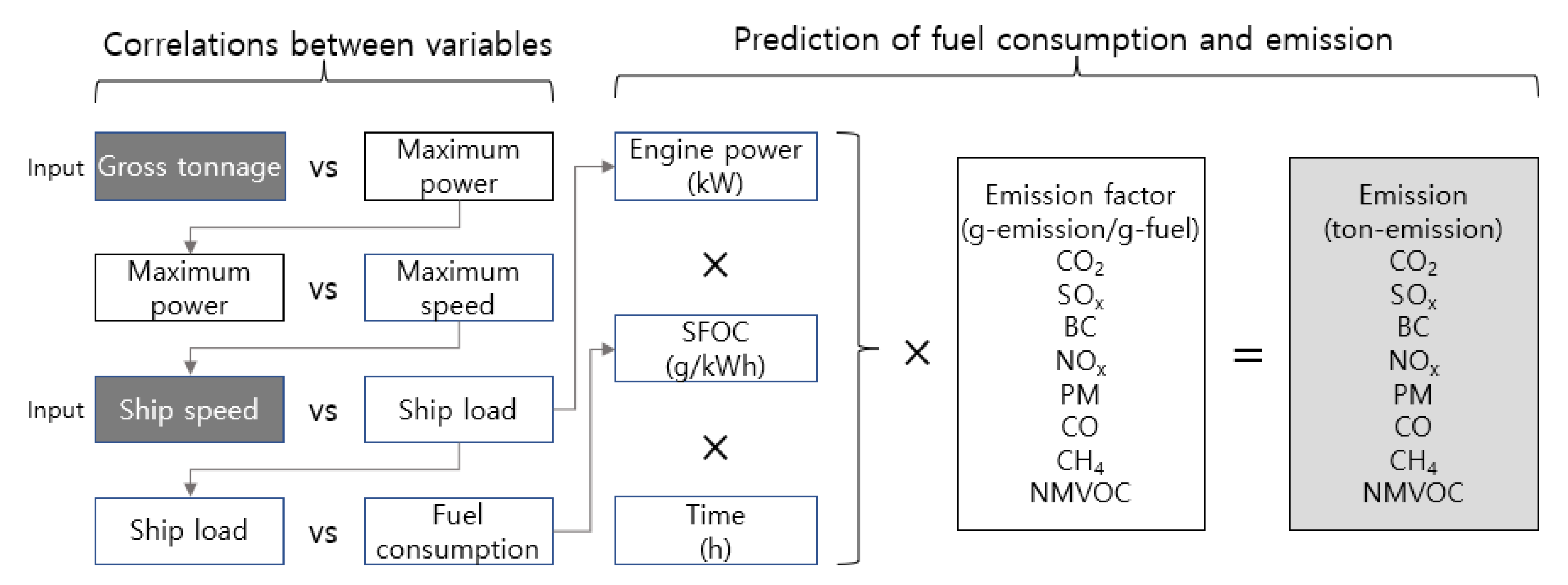
EFs must be inevitably used to calculate air pollutant emissions according to the vessel speed based on fuel properties and consumption. As changes in fuel consumption and engine power, owing to the vessel speed change, cannot be identified for each ship, it is necessary to derive this fuel consumption and engine power of individual ships through the PORT-MIS and GICOMS. Figure 5 shows the procedure in which the correlation between each variable is used in the emission calculation process. As each ship type has constant shape and speed characteristics, it was necessary to distinguish the correlations for the fuel consumption per type.

The correlations between variables required to predict fuel consumption through the gross tonnage information for each ship type included the correlation between gross tonnage and the maximum engine power; that between the maximum power and maximum speed; that between the speed and load; and that between the load and fuel consumption.

For the analysis of correlations between variables, the gross tonnage, power, speed, load, and fuel consumption were sectioned per ship type, and the correlation formulas between variables were derived through linear and polynomial regression analyses. Thus, we limited our analysis to ship types participating in the VSRP.

Figure 6 shows the correlation between the gross tonnage and power per ship type. Although the slope varies with the ship type, the power increases as gross tonnage increases. Apart from LNG carriers, the value of the coefficient of determination (R2) of the linear regression equation obtained from gross tonnage and power was significantly strong as the coefficient of determination (R2) was higher than 0.6. In the case of LNG carriers, there was no significant correlation between gross tonnage and power as the R2 value was 0.1604. This is because the sample group of LNG carriers is smaller than that of other ship types. From Figure 3, ships between 100,000 and 120,000 tons mainly made port entries for LNG carriers, as well as the sample group for the correlation analysis. Although the sample group was small, the correlation between gross tonnage and power for LNG carriers can be used as they are similar in size to LNG carriers that enter Korean ports.

Figure 7 shows the correlation between maximum power and maximum speed by ship type. Container carriers consumed the highest power, followed by crude oil, car, LNG, general cargo ships, and chemical carriers. Moreover, container carriers exhibited the highest maximum speed, followed by car carriers, LNG carriers, general cargo ships, chemical carriers, and crude oil carriers. For all ship types, the maximum speed strongly correlated with the power consumed.

Figure 8 shows the correlation between speed and load per ship type. As the load was proportional to the third power of the speed, the correlation between the speed and load was strong for all ship types, with an R2 higher than 0.9. The relationship between load and fuel consumption depends on the performance of the engine mounted in each ship. Continuous management is required for the fuel consumption of an engine to maintain the design performance. In this study, an engine-design-based SFOC was examined and applied to identify the relationship between load and SFOC. The IMO GHG study of 2014 classifies the generations of internal combustion engines for energy efficiency by ship-building year and applies baseline SFOC, as shown in

Table 1. Baseline SFOCs for marine diesel engines.

	Engine Age	Baseline SFOC [g/kWh]
		SSD	MSD	HSD
Generation 1	Before 1984	205	215	225
Generation 2	1984–2000	185	195	205
Generation 3	After 2000	175	185	195

[23].

Figure 9 shows the number of port entries for each engine generation by shipbuilding year for the target ships among the ships that entered major Korean ports in 2020. Generation 3 had the highest proportion (82%), followed by Generation 2 (17.6%) and Generation 1 (0.4%). Furthermore, container carriers represented 43% of all ship types, product/chemical carriers represented 24%, and general cargo ships (bulk carrier) 26%. Generation 3 engines were used most because they were built after 2000.

The IMO presented the SFOC by engine load according to the baseline SFOC as shown in Equation (1).

$$SFO{C}_{load}=SFO{C}_{baseline}\left(0.455\times loa{d}^2-0.71\times load+1.28\right)$$

(1)

Figure 10 illustrates the comparisons of SFOC results per load obtained by applying the baseline SFOCs for each engine generation derived through the application of the engine generation proportions in Figure 9. An SFOC curve close to 175 g/kWh was derived because most ships entering major Korean ports contain three engine generations, and the SFOC was derived as shown in Equation (2).

$$SFO{C}_{load}=80.4804\times loa{d}^2-125.58\times load+226.406$$

(2)

Table 2. Coefficients of the fitting curve by ship type obtained using the polynomial regression analysis.

Ship Type	Correlation	Coefficient			Unit
		a(x2)	b(x)	C
Container carrier	GT ∝ P	-	0.3917	13.075	[kW]
	P ∝ S	-	0.00009	18.45	[kts]
	Load diagram	1.2784	−0.4992	0.0603	[%]
	SFOC	80.4804	−125.58	226.406	[g/kWh]
	L ∝ S	−1.4924	2.407	0.0378	[%]
General cargo (Bulk carrier)	GT ∝ P	-	0.2508	1574	[kW]
	P ∝ S	-	0.0005	11.11	[kts]
	Load diagram	1.3339	−0.4908	0.0537	[%]
	SFOC	80.4804	−125.58	226.406	[g/kWh]
	L ∝ S	−1.3306	2.2725	0.0201	[%]
Car carrier	GT ∝ P	-	0.1271	6425	[kW]
	P ∝ S	-	0.0006	12.06	[kts]
	Load diagram	1.2791	−0.394	0.0418	[%]
	SFOC	80.4804	−125.58	226.406	[g/kWh]
	L ∝ S	−1.1993	2.1023	0.0569	[%]
Crude oil carrier	GT ∝ P	-	0.1432	4201	[kW]
	P ∝ S	-	0.00,006	14	[kts]
	Load diagram	1.3269	−0.4432	0.0474	[%]
	SFOC	80.4804	−125.58	226.406	[g/kWh]
	L ∝ S	−1.248	2.1643	0.0303	[%]
Chemical/Product carrier	GT ∝ P	-	0.2078	2270	[kW]
	P ∝ S	-	0.00005	18.34	[kts]
	Load diagram	1.4778	−0.6522	0.0807	[%]
	SFOC	80.4804	−125.58	226.406	[g/kWh]
	L ∝ S	−1.4802	2.4008	0.0248	[%]
LNG carrier	GT ∝ P	-	0.166	6568	[kW]
	P ∝ S	-	0.003	12.06	[kts]
	Load diagram	1.3512	−0.4572	0.0453	[%]
	SFOC	80.4804	−125.58	226.406	[g/kWh]
	L ∝ S	−1.3036	2.2456	0.0084	[%]

shows the coefficients per ship type obtained using the regression equations derived from the correlations between the variables shown in Figure 6, Figure 7, Figure 8, Figure 9 and Figure 10. Equation (2) is commonly applied for SFOC, and the other coefficients for the correlations between variables are sectioned per ship type.

3.2. Emission and Reduction Algorithm

Figure 11 shows the block diagram of the procedure for calculating the emissions and reductions of each pollutant by predicting the speed with and without speed reduction using information in applications (ship type and MMSI) and locations of ships participating in the VSRP. The input data included ship type, gross tonnage, speed, distance, and EFs.

The first step in the emission calculation (Ⓐ) in the Figure 11 is the classification of the ship type. Depending on the ship type, different coefficients were applied for the correlations between the variables, as shown in Table 2. For each ship type, the fuel consumption and engine power were deduced based on the gross tonnage information and speed. This procedure was applied to each individual vessel as follows:

• The maximum power was calculated by substituting the gross tonnage according to the correlation between gross tonnage and power.
• The maximum speed was calculated by substituting the maximum power based on the correlation between the power and speed.
• The current load was estimated by substituting the ratio of the current speed to the maximum speed into the correlation between speed and load.
• The SFOC was determined by substituting the load based on the correlation between load and SFOC.
• The power under the current load was obtained by multiplying maximum continuous rating (MCR)-power by the load.
• The time for the distance traveled was deduced based on the speed.

The second step was to determine compliance with the VSR and calculate the emissions based on the average speed by section for the target ships. In addition, emissions were obtained by estimating the speed of ships that did not comply. For such ships, the SFOC, power and time were estimated based on the MCR speed, which is the cruising speed of the ship. Finally, substances that apply energy-based EFs and fuel-based EFs were divided to explore EFs. Energy-based EFs were expressed in g-emission/kWh by multiplying power and time, and fuel-based EFs were expressed in g-emission/g-fuel by multiplying SFOC, power, and time.

4. Emission Factor Calculation

In this study, we utilized the EFs presented by the 2020 IMO GHG study. The IMO presents fuel-based and energy-based EFs separately. Fuel-based EFs (g-emission/g-fuel) are expressed as emissions (g) when 1 g of fuel is consumed, and energy-based EFs (g-emission/kWh) are expressed as emissions (g) for power generated per unit time. The substances classified as EF-fuel were CO₂, SOx, and black carbon (BC), whereas those classified as EF-energy were NOx, PM, methane (CH₄), CO, nitrous oxide (N₂O), and NMVOC. EFs are used differently, depending on the type and sulfur content of the fuel oil, engine stroke type, engine speed, and engine production year. In this study, emissions were assessed using gross tonnage and speed information for the target ships of the VSRP only; thus, detailed information could not be identified. Therefore, for the fuel oil and sulfur content, a heavy fuel oil (HFO) with a sulfur content of 0.5% m/m, which is the fuel oil mainly used by the target ships, was assumed. For the engine type, a low-speed marine two-stroke diesel engine was assumed for the EF calculation.

4.1. Fuel Based Emission Factors

The IMO presents the CO₂ conversion factor per fuel type based on the 2018 EEDI Guidelines [24].

Table 3. Conversion factor between fuel consumption and CO₂ emission.

Type of Fuel		LCV (kJ/kg)	Carbon Content	CF (t-CO2/t-Fuel)
Diesel/Gas Oil		42,700	0.8744	3.206
LFO		41,200	0.8594	3.151
HFO		40,200	0.8493	3.114
LPG	Propane	46,300	0.8182	3.000
	Butane	45,700	0.8264	3.030
LNG		48,000	0.7500	2.750
Methanol		19,900	0.3750	1.375
Ethanol		26,800	0.5217	1.913

outlines the conversion factor per fuel type used. The CO₂ conversion factor varies with the calorific value and carbon content of the fuel. In this study, the conversion factors for HFO were used.

SO_x emissions varied with the sulfur content of the fuel or use of an exhaust gas cleaning system. For ships entering Korean ports, a global sulfur content of 0.5% m/m or less should be used under the MARPOL regulation, while those with sulfur content of 0.1% m/m should be used during anchoring, according to the special law on air quality improvement in port areas. As emissions were determined when ships traveled in speed reduction zones in this study, they were based on HFO with a sulfur content of 0.5% m/m. Equation (3) shows the conversion factor of SO_x according to the sulfur content of fuel presented in the Third IMO GHG Study 2014 [23] and by Olmer et al. [25].

$$gS{O}_x=gfuel\times 2\times 0.97753\times fuelsulfurfraction$$

(3)

BC was estimated by multiplying the fuel consumption by EF in a manner similar to that of CO₂. The BC emissions were higher when residual oil was used than when distilled oil was used. Equation (4) shows the conversion factor calculation curve for BC according to the engine load calculated based on the residual oil used on ship. This was demonstrated by Comer et al. [26].

$$B{C}_{2-stroke}\left(g/kgfuel\right)=0.1500\times loa{d}^{-0.359}$$

(4)

4.2. Energy-Based Emission Factors

Energy-based EFs are conversion factors used to calculate the emissions of each substance based on the engine power (kW) and time of use by the shipload.

Table 4. Energy-based emissions factors for NOx.

Engine Type	HFO, LSHFO & MDO EF NOx (g NOx/kWh)
	Tier 0	Tier 1	Tier 2	Tier 3
SSD	18.1	17.0	14.4	3.4
MSD	14.0	13.0	10.5	2.6
HSD	10.0	9.8	7.7	2.0

outlines the conversion factors of diesel engines for NO_x. NO_x regulations have been applied in stages: Tier 3 is being applied in ECA while Tier 2 in areas other than ECA. As Korea does not belong to the ECA, up to Tier 2 were applied to ships. Tier 0 was applied to ships built before 2000, Tier 1 to ships built before 2011, and Tier 2 to ships built after 2011.

Figure 12 shows the number of ships subject to NO_x levels by ship types and building years for the target ships of the VSRP that entered major Korean ports in 2020. Tier 0, Tier 1, and Tier 2 accounted for 18%, 24%, and 34%, respectively. In this study, the EF of NO_x was selected by considering the proportion of port entries.

Equation (5) is a function of the fuel consumption and sulfur content presented by the IMO to calculate the PM of a ship using HFO. The level of PM varies depending on the presence or absence of a scrubber device, fuel consumption, and sulfur content of the fuel. In this study, the installation of a scrubber device on each ship could not be performed; thus, it was not considered.

$$PM\left(\frac{g}{kWh}\right)=1.35+SFOC\left(\frac{g}{kWh}\right)\times 7\times 0.02247\times \left(fuelsulfurfraction-0.0024\right)$$

(5)

Figure 13 illustrates the results of deriving PM based on the load by substituting HFO with a sulfur content of 0.5% m/m and Equation (1) for inducing SFOC by engine efficiency into Equation (5). The latest engines generated low PM emissions, and the optimal operating load to minimize PM emissions was approximately 80%. The black-derived curve illustrates the results of the PM derived by considering the engine generation of ships that entered major Korean ports.

Table 5. Energy-based emissions factors for different engine types and all fuels.

Engine Type	Fuel Type	CH4 (g/kWh)	CO (g/kWh)	N2O (g/kWh)	NMVOC (g/kWh)
SSD	HFO	0.01	0.540	0.031	0.632
	MDO	0.01	0.044	0.030	0.632
MSD	HFO	0.01	0.540	0.034	0.527
	MDO	0.01	0.046	0.030	0.527
HSD	HFO	0.01	0.540	0.030	0.527
	MDO	0.01	0.540	0.034	0.527
LNG–Otto (DF, MS)	LNG	5.5	1.3	0.020	0.500
LNG–Otto (DF, SS)	LNG	2.5	1.3	0.020	0.500
LNG–Diesel (DF)	LNG	0.2	1.04	0.030	0.400

shows the EFs of CH₄, CO, N₂O, and NMVOC per engine and fuel types. Unlike NO_x and PM, the same value was applied for engine generation and EFs were obtained differently per engine type.

Unburnt methane is discharged from diesel engines and engines that use LNG, owing to methane slip. The emission of methane increased significantly with the consumption of LNG. In international transport, the total LNG consumption increased by 28% to 30% between 2012 and 2018, while the emission of methane increased by 151–155% during the same period. This is because LNG fuel was gradually expanded to general ships to respond to the emission regulations of the IMO.

The EF of methane was published by the Fourth IMO GHG Study and Jorgen et al. [27]. Diesel engines that used HFO and marine diesel oil (MDO) have the same EF for unit power. For engines that used LNG fuel, low-pressure injection engines that adopt the Otto cycle used a higher EF than high-pressure injection engines that adopted the diesel cycle. This is because the methane slip that escapes through the exhaust value occurs in the Otto cycle, whereas the fuel is injected during the intake process for premixed combustion.

CO is one of the four major air pollutants generated by diesel engines, alongside HC, NO_x, and PM. CO is generated by the incomplete combustion of carbon. It is a colorless and odorless gas. CO is inhaled and delivered into the bloodstream. Therein, it inhibits the oxygen-carrying capacity of the blood by combining with hemoglobin. CO can cause suffocation depending on its concentration in air, thereby affecting the functioning of human organs [28,29].

N₂O is one of the six gases first considered in the United Nations Framework Convention on Climate Change (UNFCCC) process: CO₂, CH₄, N₂O, hydrofluorocarbons, perfluorocarbons, and sulfur hexafluoride. N₂O causes ozone layer depletion and contributes to the greenhouse effect and has attracted increased attention recently because of its ever-increasing concentration in the atmosphere [30].

NMVOC is a non-combustion emission that occurs during the loading, unloading, and transport of fuel and crude oils.

5. Results

In this section, the emission and reduction of container carriers among the ships participating in VSRP in 2020 were assessed using the algorithm and EFs as illustrated in Section 2 and Section 3. In addition, the results of this study were verified by comparing the average power, speed, fuel consumption, and CO₂ emissions of the global container fleet in 2018, according to the IMO, using the bottom-up method.

Figure 14 illustrates the statistics of ships participating in the VSRP per type among ships that entered major Korean ports in 2020. Container carriers accounted for 90.1% of all the ships, and the other ship types represented approximately 10%. The emission calculation algorithm derived in the previous section was applied to the container carriers. In 2020, the number of container carriers that applied for participation in the VSRP in Korea was 9451. Among them, the number of ships that complied with the target speed of 12 knots was 8887 and the number that did not comply with the target speed was 564. Among the 9451 ships, the average speed of the ships that complied was 9.5 knots, while that of the ships that did not comply was 12.6 knots.

Table 6. The amount of air pollutant reduction in the container fleet through the VSRP.

	Real Speed Condition			Cruising Speed Condition			Amount of Reduction
	Total	Average		Total	Average		Total	Average
Time [h]	21,097	2.23	-	9115	0.96	-	−11,981	−1.27	−131%
Power [kW]	26.2 × 106	2769	-	233.6 × 106	24,736	-	207.5 × 106	21,967	88%
Fuel consumption [ton]	10,871	1.15	-	38,686	4.10	-	27,815	2.94	71.9%
Speed [kts]	-	9.6	-	-	17.9	-	-	-	47%
Emission	[ton]	[kg/ship]	[%]	[ton]	[kg/ship]	[%]	[ton]	[kg/ship]	[%]
CO2	33,852.4	3583.40	97.1	120,469.0	12,752.09	96.6	86,616.6	9168.7	71.9
SOx	108.5	11.48	0.311	386.0	40.86	0.309	277.5	29.4	71.9
BC	2.9	0.31	0.008	10.3	1.09	0.008	7.4	0.8	71.9
NOx	838.0	88.71	2.403	3534.4	374.13	2.834	2696.3	285.4	76.3
PM	16.1	1.71	0.046	67.9	7.19	0.054	51.8	5.5	76.3
CH4	0.5	0.05	0.001	2.2	0.23	0.002	1.7	0.2	76.3
CO	27.7	2.94	0.080	116.0	12.38	0.094	89.3	9.4	76.3
N2O	1.6	0.17	0.005	6.7	0.71	0.005	5.1	0.5	76.3
NMVOC	32.5	3.44	0.093	136.9	14.49	0.110	104.5	11.1	76.3

shows emissions from the container carriers participating in the VSRP and their degree of reduction. All the ships consumed 10,871 tons of fuel while traveling for 21,097 h in the speed reduction zones. On average, one ship consumed 1.15 tons of fuel while traveling approximately 2.2 h at 9.6 knots. When the cruising speed was predicted and calculated under the condition of non-participation in the VSRP, the cruising speed was 17.9 knots and the total fuel consumption was 38,686 tons. As the cruising speed was higher than that for VSRP, the travel time in the speed reduction zones reduced to 11,981 h. Moreover, the power decreased by 88% and the fuel consumption by 71.9% as the speed decreased by 47%. In the case of the emissions reduction, fuel-based emissions (CO₂, SO_x, and BC) decreased by 71.9% and energy-based emissions (NO_x, PM, CH₄, CO, N₂O, and NMVOC) decreased by 76.3%.

Figure 15 shows the distribution of CO₂ emissions from container carriers based on their gross tonnage obtained from Table 6. Among all container carriers, vessels with a gross tonnage between 3000 and 10,000 tons exhibited the highest proportion (38.3%), while most of the vessels (78.4%) had a gross tonnage of 60,000 tons or less. The CO₂ emissions and reductions were proportional to the number of vessels. The CO₂ emissions per ship also increased as the gross tonnage, with the difference ranging from 5.3% to 10.1%. The CO₂ reduction per ship also increased with the gross tonnage. Container carriers with a gross tonnage between 3000 and 10,000 tons accounted for approximately 2.3% of the total reduction, but those with a gross tonnage between 220,000 and 240,000 tons represented 13.7%, achieving a reduction effect approximately six times higher.

To verify the reliability of the algorithm developed for predicting fuel consumption based on the gross tonnage and vessel speed by ship type, the results obtained were compared with that of the average maximum power and fuel consumption by TEU, presented by the IMO through the statistics of the container fleet in 2018.

Table 7. Comparison of fuel consumption between IMO-presented container fleet and the algorithm-applied container ship.

Container		No. of Vessels	Average Value for 2018 Describing the Fleet Analyzed Using the Bottom-Up Method by IMO					The Value Derived from the Algorithm of This Study
			MCR	Design Speed	SOG. at Sea	Fuel	Fuel Consump.	MCR	Design Speed	Assumed SOG	Fuel Consump.
Case	Teu	No.	kW	kn	kn	kt	ton/h	kW	kn	kn	ton/h
A	1000–1999	1271	12,083	19.0	13.4	5.1	0.53	13,858	19.6	13.4	0.84
B	2000–2999	668	20,630	21.1	14.2	7.9	1.00	20,565	20.3	14.2	1.34
C	3000–4999	815	34,559	23.1	14.7	12.7	1.49	34,544	20.3	14.7	2.12
D	5000–7999	561	52,566	24.6	15.7	20.3	2.13	52,243	21.6	15.7	3.16
E	8000–11,999	623	57,901	23.9	16.3	26.4	3.27	57,746	23.1	16.3	3.63
F	12,000–14,499	227	61,231	23.8	16.3	27.2	4.19	63,448	23.6	16.3	3.79

compares the results of fuel consumption usage of container ships announced by IMO and the results of fuel consumption calculated through the algorithm of this study. For comparison with the results of the IMO fleet, A–F cases used a sample of container ships participating in Korean VSRP with similar MCR power in each case. Fuel consumption calculated by the algorithm during operation was compared with SOG, which is the same as the average speed of the IMO fleet of A–F cases.

Figure 16 illustrates the comparison of CO₂ emission results between the IMO and the algorithm for cases A–F in Table 7. For case A, an IMO ship with a power of 12,083 kW had an MCR speed of 19.0 kts and it consumed 1 kton of fuel on average per year while traveling at 13.4 kts on average. The fuel consumption per hour was estimated to be 0.53 tons/h. For a ship with a similar power of 13,858 kW among the container ships participating in Korea’s VSRP, the MCR speed derived by the algorithm was 19.6 kts, resulting in a difference of approximately 0.6 kn. Assuming a vessel speed of 13.4 kts, the fuel consumption was estimated to be 0.84 ton/h, resulting in a difference of approximately 0.29 ton/h. A comparison with IMO ships corresponding to cases B, C, and D showed good agreement with an error of less than 10% in terms of the CO₂. For cases E and F, errors of approximately 13% and 18% occurred in predicting fuel consumption and CO₂ emissions, respectively. When looking at the slope of the connection between the output and the case for CO₂, it can be seen that the result of the CO₂ emission is similar to a ship with relatively smaller power.

This could be explained by the difference in the number of target ships in relation to tonnage range between the IMO ships and the ships used for the development of the algorithm. The variables used to calculate fuel consumption, in particular, are considered to be the difference that occurs in the correlation between the gross tonnage, power, and speed of Figure 6a and Figure 7a. However, the effect of this on the error in total emissions decreases because more than 90% of the container ships entering Korean ports are ships of 50,000 kW or less. Therefore, the developed algorithm can accurately estimate the emissions from container ships of 50,000 kW or less. However, fuel-based EFs can be verified using the fuel consumption of the statistical fleet presented by the IMO. Since there is no output of vessel speed, the verification of NO_x, PM, CH₄, CO, N₂O, and NMVOC may have limitations. As fuel consumption is based on the unit power and time, the actual fuel consumption is assumed to be similar to the consumption presented in the statistics.

6. Discussion

To estimate emissions from ships participating in the VSRP that enter major Korean ports, we developed an algorithm for predicting the fuel consumption based on the gross tonnage and vessel speed by ship type. In addition, the conversion factors presented by the IMO were applied according to the domestic situation by reflecting information, such as the fuel used by ships entering domestic ports, the sulfur content according to the local regulation, and the ship age. We presume that further research will be conducted on the construction of a system that predicts emissions more accurately by continuously recording the emissions from ships participating in Korea’s VSRP and the degree of reduction in a database using our present algorithm. In this section, the limitations and improvements of the developed algorithm and the application of EFs are presented and the future research directions set.

The emission sources of ships can be divided into Aux. Engine and Aux. Boiler. Figure 17 shows the power of the Aux. Engine and Aux. Boiler in ship operation condition for dead weight of container ships. The generator engine of a container ship consumes the lowest power at berth and the highest power during maneuvering. This is because devices related to the main engine required for navigation do not operate at the berth. Moreover, only one generator engine operated as minimum electric power was required for residential facilities. This is also because there was no loader for loading and unloading cargo, owing to the nature of the container ships.

During entry into and departure from a port, two or more generator engines prepare for the operation of the bow thruster and emergency situations at the port. During anchoring, the main engine is not involved but the standby state is maintained so that it can be used. Thus, the power consumption is similar to that during navigation. The boiler is used to heat the bunker oil, which is stopped during navigation because the exhaust gas boiler is in operation. The use of the boiler was almost the same at the berth and during the anchoring. The exhaust gas boiler operated during port entry and departure, owing to the exhaust gas of the main engine. As the power of the main engine was very low, Aux., the boiler continuously operated to exhibit a power similar to that at berth or during anchoring.

Figure 18 shows the ratios of the auxiliary engine power and boiler power to the main engine power by the operation mode. The ratio increased as the ship size decreased for all operation modes. For ships with a dead weight of 75,000 or higher, the Aux. engine power and boiler power to the main engine power were similar. Although a direct comparison of emissions from the main engine through Figure 18a,b was difficult, emissions from the generator engine ranged from 2.0% to 15.6% when compared to the main engine power. In the case of the Aux. boilers, emissions ranging from 1.0% to 4.9% should be considered, except for maneuvering. As our algorithm was applied to the target ships of the VSRP entering Korean ports, the low-speed operation corresponded to the maneuvering speed. Therefore, the total emissions from ships can be derived if the fuel consumption for the loads of Aux. engine and boiler are considered.

The most important factor in determining emissions using EFs is by using the SFOC curve. The SFOC differs depending on the engine stroke type (two-stroke and four-stroke), engine type (diesel, steam turbine, and gas turbine), engine speed (slow speed diesel (SSD), medium speed diesel (MSD), and high speed diesel (HSD)), fuel type (HFO, MDO, MeOH, and LNG), and engine production year (before 1983, 1984–2000, and after 2001). In this study, the statistics of the tonnage and production year of ships entering Korean ports were used to eliminate the limitation of not being able to secure information about individual ships; therefore, errors may have occurred. Although large errors may occur for individual ships, emissions can be accurately estimated as the number of target ships increases, because regression models were applied based on the specifications of 1420 container ships and the models presented based on the statistics of the IMO.

The variables affecting ship operation that were not considered in this study include the hull-fouling factor, weather correction factor, and hull draught.

As the hull becomes rough due to continuous biofouling after dry-docking, it is necessary to apply the fouling coefficient to obtain the hull resistance. According to a study, the power of the main engine can be increased by 7% on an average, depending on the deterioration of the ship and maintenance schedule [25]. The hull must be maintained through two docking inspections within five years, according to regulations. This means that hull fouling occurs over two to three years after docking. Therefore, it is necessary to apply a hull-fouling factor accordingly.

The influence of weather on the propulsion force of a ship is determined by the wave height and direction as well as the wind intensity and direction. Considering the increase in hull resistance, reflecting the environmental conditions of waves and wind requires an algorithm to determine the effect of weather conditions on fuel consumption. As the environmental data used can have significant uncertainties, further research is recommended to apply additional weather factors.

The draught of a ship varies depending on the amount of cargo loaded. If the draught is reduced, the required propulsion force decreases owing to the reduction in the contact area with the water surface. For bulk carriers, general cargo ships, and tankers, full loading and unloading cause significant changes in draught because they mostly carry single cargo. However, in the case of container carriers and car carriers, the application of the average draught value is acceptable, as the draught varies with the amount of cargo; however, it causes no significant change in draught. In the Third IMO GHG Study, the draught adjustment factor was simply the annual average draught divided by the design draught to 2/3 power for ships with constant draught [23]. For an accurate emission estimation, we divided the ship types according to the applicability of the average draught factor and we applied different draught factors.

An additional factor to consider is the effect of the methane slip. Owing to the reinforcement of the MARPOL agreement, more LNG-powered ships have been introduced to satisfy NOx and SOx regulations. LNG-powered ships can be divided into diesel cycle engine types (that perform combustion through high-pressure injection) and the Otto cycle engine type (that performs combustion through low-pressure injection). For LNG-fueled engines that use the Otto cycle, the methane slip of approximately 5% of the injection amount occurs [31]. In the case of dual fuel (DF) engines that adopt a diesel cycle, the methane slip of approximately 0.2% occurs. Currently, orders for LNG-powered ships are increasing worldwide, but most operating ships are diesel-powered. The increase in LNG-powered ships should be considered in future studies.

7. Conclusions

The VSRP was introduced and implemented in major Korean trade ports in December 2019 to improve port air quality. This study aimed at estimating the emissions from ships participating in the VSRP and the degree of emission reduction effect due to the program. Therefore, in this study, an emission prediction algorithm was developed, and the conclusion is as follows.

• We developed an algorithm for calculating the fuel consumption and power based on the actual vessel speed, and the total emissions were calculated using the bottom-up approach. The contents developed in this study were applied to the emission program of an automatic verification system of the VSRP. For the correlations between the variables used in the algorithm, we utilized the detailed design specifications of ships registered in the KR and KOMSA. The input of the algorithm reflects the AIS data of the GICOMS and the port entry and departure information of the PORT-MIS. Thus, we derived the emissions and the degree of emission reduction for container ships that participated in the VSRP in 2020.
• The container ships consumed 10,871 tons of fuel while traveling at 9.6 knots on average for 21,097 h in the speed reduction zones. When the cruising speed was estimated when ships did not participate in the VSRP, it was predicted that the ships would consume 38,686 tons of fuel while traveling at 17.9 knots on average for 11,981 h in the same zones, indicating a 71.9% CO₂ reduction effect due to the speed reduction by 47%.
• For the verification of the algorithm, the fuel consumption of the container fleet presented by the IMO was compared with the fuel consumption derived through the algorithm for cases A–F. Case A showed a difference of approximately 0.29 tons/h at the same speed, while cases B, C, and D exhibited an error of less than 10% in fuel consumption at the same speed. Cases E and F showed an error of approximately 13% in the fuel consumption at the same speed. In cases B, C, and D, where more than 90% of ships participating in VSRP correspond, CO₂ emissions showed good agreement with IMO cases. As a result, the comparative results were more suitable for container ships with relatively low power than for ships with high power.

In this study, the emission amount is calculated by estimating the fuel consumption and power corresponding to the gross tonnage and speed of individual ships, rather than the top-down method of the emission of a group of ships entering Korean ports annually. Therefore, the application of the algorithm in this study is considered to be different from the existing emission calculation method.

The developed algorithm reflects only the fuel consumption and power of the main engine; thus, it is necessary to apply an algorithm that can determine total emissions, including that from the auxiliary engine and boilers, to the automatic verification system of the VSRP. The results of this study can be used to monitor the effect of air pollutant emissions from ships entering major ports in Korea and can be used in developing policies envisaged at reducing greenhouse gases and air pollutants. Therefore, we suggest that this algorithm be used in other countries for monitoring ship-induced emissions.