Modeling of Vehicle-Mounted Flywheel Battery Considering Automobile Suspension and Pulse Road Excitation

Abstract

The existing model of magnetic suspension force for flywheel batteries mainly focuses on the internal magnetic field and foundation motions. However, when applied to vehicle-mounted occasions, the accuracy of the model will inevitably be affected by the vehicle vibration system and road conditions. Therefore, in view of the shortcomings of the existing research, a typical road condition (pulse road excitation) is taken as an example in this study to establish a model of magnetic suspension force that comprehensively considers automobile suspension and pulse road excitation. First, on the basis of a static model for magnetic suspension force using the equivalent magnetic circuit method, a magnetic suspension force dynamic model that takes into account the influence of automobile suspension and pulse road excitation is established. The rules of dynamic response under the influence of automobile suspension and pulse road excitation are summarized, and the foundation offset is corrected in the form of main migration points. Therefore, a correction model of magnetic suspension force is established. Finally, performance tests are carried out. The better anti-interference capability of the correction model is proven by the experimental results.

1. Introduction

Flywheel batteries, a new concept of energy storage devices, push the limits of chemical batteries and achieve physical energy storage through the high-speed rotation of a flywheel [1,2,3]. After years of development, flywheel energy storage technology has become relatively mature and is widely used in various scenarios, including electric vehicles [4,5,6,7]. However, when applied to vehicle applications, the stability of a magnetic bearing–flywheel system will be reduced by the additional disturbances from the vehicle vibration system (such as the automobile suspension), foundation motion (namely driving conditions), road conditions, etc. Furthermore, as the key component for achieving stable operation, flywheel batteries have strict requirements for the magnetic bearing–flywheel system [8,9,10]. Therefore, it is necessary to comprehensively consider the influence of additional vehicle-mounted disturbances and establish an accurate mathematical model of magnetic suspension forces.

The existing model of magnetic suspension force for flywheel batteries mainly focuses on the internal magnetic field and foundation motions [11,12,13]. In [11], a magnetic suspension force modeling method based on precise magnetic field segmentation is proposed, taking into account the fringing flux and the leakage flux, but the method still falls within the scope of static modeling. Furthermore, in [12], a multidimensional dynamic magnetic suspension force modeling method based on the temperature and rotating speed is proposed, taking into account the deformation caused by high-speed rotation and temperature changes. In [13], a dynamic correction model considering basic foundation motion is proposed, which covers multiple common driving conditions, such as acceleration, turning, uphill, etc. However, considering the complexity and diversity of additional disturbances under vehicle-mounted conditions, it is clearly not enough to only consider the influence of foundation motion.

However, in terms of vehicle vibration systems, the existing research has mainly taken the vibration system as a supplementary condition, and thus, the dynamic performance of a magnetic suspension system can be analyzed more comprehensively [14,15]. In [14], in order to verify the robustness of a designed sliding-mode controller, a vehicle-mounted flywheel battery was placed on a spring shock platform (as a simplified automobile suspension system) for road performance tests. In [15], in order to suppress the influence of base excitation on a magnetic bearing system, a magnetic bearing–rotor system placed on a spring-base system (as a simplified damping system) was taken as an example, and the compensation effect of the proposed BAFC algorithm was verified.

In terms of road conditions, the existing studies have mainly focused on the influence of road conditions on the dynamic performance of a magnetic suspension system [16,17,18]. In [16], in order to verify the feasibility of a designed traction system, an integrated flywheel energy storage system was taken as an example, and the dynamic response of the flywheel under the action of road surface friction was analyzed. In [17], in order to explore the influence of irregular road conditions, an active magnetic bearing for a vehicle-mounted flywheel battery was taken as an example, and the dynamic performance of a magnetic suspension system was analyzed. The results showed that in order to adapt to complex road conditions, it was necessary to make additional design and controller modifications in the magnetic suspension system. In [18], in order to analyze the dynamic performance of a magnetic suspension system, an active magnetic bearing was taken as an example. The results showed that the stiffness and damping of the magnetic bearing were reduced under the influence of road excitation, which provided a basis for the design of a magnetic suspension support system.

In summary, the accuracy of a magnetic suspension force model will be affected by additional disturbances under vehicle-mounted conditions (including the vehicle vibration system, foundation motion, and road conditions). However, the existing modeling methods mainly focus on the research of internal magnetic fields, while there has still been little research on the influence of vehicle-mounted disturbances on the magnetic suspension force model. In terms of vehicle vibration systems and road conditions, most studies have also been limited to dynamic performance analysis, without further considering the stage of modeling. Therefore, in view of the shortcomings of the existing research, the purpose of this study was to comprehensively consider the influence of automobile suspension and typical road conditions (pulse road excitation) and further improve the magnetic suspension force model, taking into account the vehicle-mounted conditions.

In this study, taking a vehicle-mounted flywheel battery as an example, a magnetic suspension force model was established considering automobile suspension and pulse road excitation. First, a static model of the flywheel battery was derived using the classical equivalent magnetic circuit method. On this basis, a dynamic model considering automobile suspension and pulse road excitation was established. Then, in order to improve the accuracy of the model, the rules of dynamic response under the influence of automobile suspension and pulse road excitation were summarized. Furthermore, the foundation offset was corrected in the form of main migration points. It is worth noting that the axial model was much more susceptible than the radial model under the influence of automobile suspension and pulse road excitation. Therefore, the axial model was taken as an example for correction in this study. Finally, performance tests were carried out to verify the superior anti-interference capability of the established correction model compared to the static model.

2. Mathematical Model and Dynamic Correction

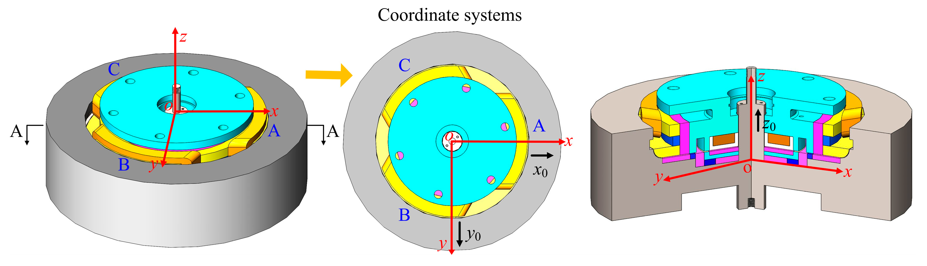
2.1. Topology

The overall topology and magnetic circuit of a three-degrees-of-freedom (3-DOF) flywheel battery with a virtual inertia spindle are shown in Figure 1. The motor and combined magnetic bearing (including a radial magnetic bearing and an axial magnetic bearing) are embedded in the flywheel, which reduces the volume of the flywheel battery and improves the integration of the system. The air gap between the radial magnetic bearing and the flywheel is spherical, which improves the anti-interference performance of the system. The bias magnetic flux is formed by two annular permanent magnets, and the control magnetic flux is formed by control coils to maintain the stable suspension of the flywheel. The bias magnetic circuit and control magnetic circuit are marked in Figure 1. Furthermore, a detailed description of the suspension mechanism and a performance analysis are presented in [19] and are not repeated here.

2.2. Static Magnetic Suspension Force Model

In order to emphasize the influence of automobile suspension and pulse road excitation on a magnetic bearing–flywheel system, a static model was established using a classical equivalent magnetic circuit method based on the magnetic circuit in Figure 1. Thus, the complexity of the model was simplified and the control efficiency was improved.

As shown in Figure 2, a reference coordinate system was established for static modeling, whose origin was located on the centroid of the flywheel. It was further assumed that the flywheel was simultaneously eccentric in both the radial and axial directions, that is, the flywheel deviated from x₀, y₀, and z₀ along the positive directions of the x-axis, y-axis, and z-axis of the reference coordinate system, respectively.

Furthermore, by using the reference coordinate system established in Figure 2, the electromagnetic forces F_A, F_B, and F_C at the radial air gap are projected onto the x-axis and y-axis, respectively. Therefore, the radial magnetic suspension force can be expressed as:

$$F_x=F_{\mathrm{A}}-\frac{1}{2}{F}_{\mathrm{B}}-\frac{1}{2}{F}_{\mathrm{C}}; F_y=\frac{\sqrt{3}}{2}{F}_{\mathrm{B}}-\frac{\sqrt{3}}{2}{F}_{\mathrm{C}}$$

(1)

where F_x and F_y are the radial magnetic suspension forces projected onto the x-axis and y-axis, respectively.

Moreover, due to the small air gap of the magnetic bearing–flywheel system, the magnetic circuit of the flywheel works in the linear region. Based on the small air gap, the complexity of the model can be further reduced: the radial magnetic suspension forces (F_x, F_y) and the axial magnetic suspension force (F_z) are linearized near the equilibrium position. Therefore, the static model can be expressed as:

$$\left\{\begin{array}{l}{F}_x\cong k_x\cdot x_0+k_{ix}\cdot i_{x0}; F_y\cong k_y\cdot y_0+k_{iy}\cdot i_{y0}\\ F_z\cong k_z\cdot z_0+k_{iz}\cdot i_{z0}\\ k_x=k_y=\frac{3{\mu }_0{F}_{m1}{}^2}{2{\delta }_r{}^3(\frac{1}{S_{r2}}+\frac{1}{S_r})}; k_{ix}=k_{iy}=\frac{2{\mu }_0{F}_{m1}{N}_1}{{\delta }_r{}^2(\frac{1}{S_{r2}}+\frac{1}{S_r})}\\ k_z=\frac{S_{a1}{\mu }_0{(F_{m2}+F_{m3})}^2}{4{\delta }_{a1}{}^3}; k_{iz}=\frac{N_2{\mu }_0(F_{m2}+F_{m3})}{2}\cdot \frac{1}{(\frac{{\delta }_{a1}{\delta }_{a2}}{S_{a2}}+\frac{{\delta }_{a1}{}^2}{S_{a1}})}\end{array}\right.$$

(2)

where k_x and k_y are the static force–displacement stiffness values on the x-axis and y-axis, respectively; k_ix and k_iy are the static force–current stiffness values on the x-axis and y-axis, respectively; k_z and k_iz are the static force–displacement stiffness and force–current stiffness values, respectively on the z-axis; x₀, y₀, and z₀ are the static offset values on the x-axis, y-axis, and z-axis, respectively; i_x0, i_y0, and i_z0 are the static control currents on the x-axis, y-axis, and z-axis, respectively; μ₀ is permeability of vacuum; N₁ and N₂ are the single-phase effective turns of the radial equivalent three-phase coils and the axial coils, respectively; F_m1, F_m2, and F_m3 are the magnetic potentials of the radial permanent magnet, axial outer permanent magnet, and axial inner permanent magnet, respectively; δ_r, δ_α1, and δ_α2 are the initial air gap lengths at the radial, axial lateral, and axial inboard, respectively; S_r, S_r2, S_α1, and S_α2 are the face areas of the radial upper stator pole, radial lower stator pole, axial lateral stator pole, and axial inboard stator pole, respectively.

2.3. Dynamic Magnetic Suspension Force Model

Obviously, the above static model does not take into account the influence of automobile suspension and pulse road excitation. However, due to the influence of these factors, the flywheel is subjected to forced vibration, resulting in the additional offset of the flywheel (defined as the foundation offset). At the same time, to compensate for the impact of the additional offset, a compensation current is produced by the control coils of the magnetic bearing–flywheel system to generate additional magnetic suspension force. Furthermore, it is worth noting that, considering the universal applicability, special circumstances of vehicle driving (such as a head-on crash or lateral tilt in extreme cases) were not considered. Therefore, the dynamic model of magnetic suspension force can be expressed as:

$$\left\{\begin{array}{l}{F}_{dx}=k_{dx}\cdot x+k_{dix}\cdot i_{x0}\\ F_{dy}=k_{dy}\cdot y+k_{diy}\cdot i_{y0}\\ F_{dz}=k_{dz}\cdot z+k_{diz}\cdot i_{z0}\\ k_{dx}=\left|\frac{x-x_0}{∆x_f}\right|k_x;k_{dy}=\left|\frac{y-y_0}{∆y_f}\right|k_y;k_{dz}=\left|\frac{z-z_0}{∆z_f}\right|k_z\\ k_{dix}=\left(1+\frac{∆i_{fx}}{i_{x0}}\right)k_{ix};k_{diy}=\left(1+\frac{∆i_{fy}}{i_{y0}}\right)k_{iy};k_{diz}=\left(1+\frac{∆i_{fz}}{i_{z0}}\right)k_{iz}\end{array}\right.$$

(3)

where Δx_f, Δy_f, and Δz_f are the foundation offset values on the x-axis, y-axis, and z-axis, respectively; Δi_fx, Δi_fy, and Δi_fz are the compensation currents generated by the control coils on the x-axis, y-axis, and z-axis, respectively; x, y, and z are the actual offset values of the flywheel on the x-axis, y-axis, and z-axis, respectively, under the influence of automobile suspension and pulse road excitation; k_dx, k_dy, and k_dz are the dynamic force–displacement stiffness values on the x-axis, y-axis, and z-axis respectively; k_dix, k_diy, and k_diz are the dynamic force–current stiffness values on the x-axis, y-axis, and z-axis, respectively.

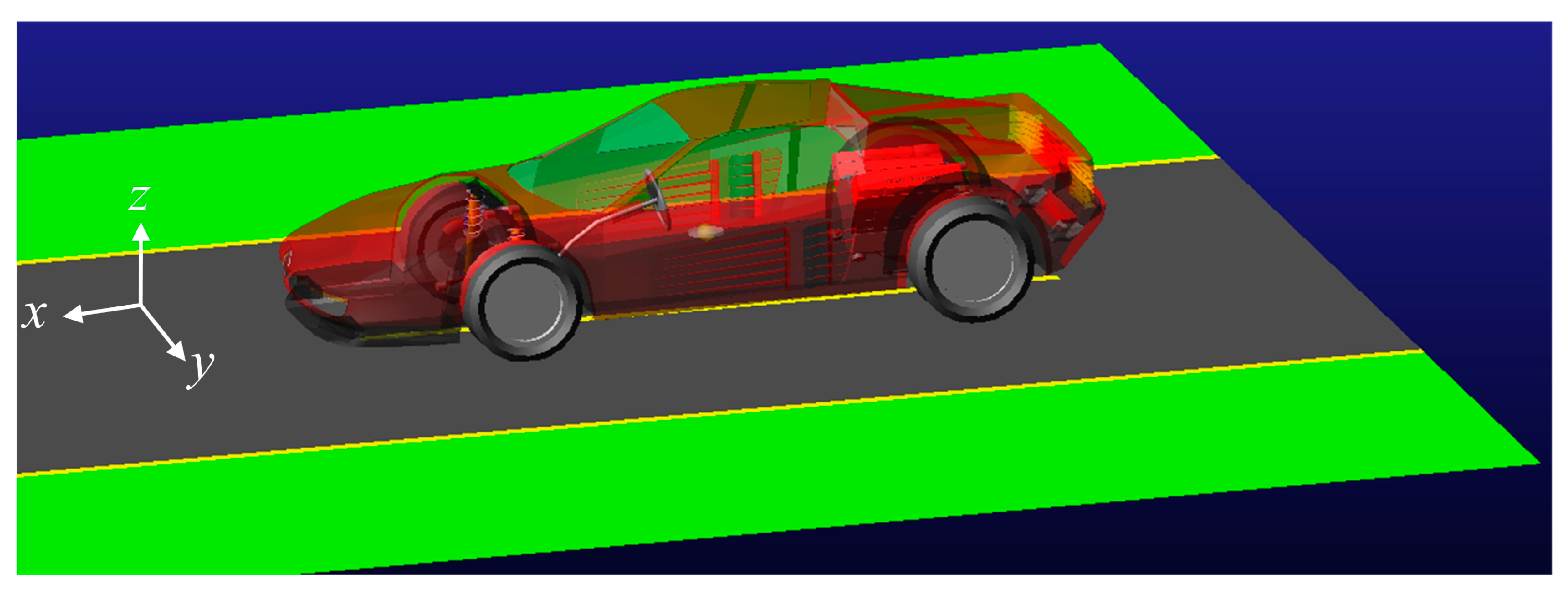
2.4. Parameters of Automobile Suspension System

Due to the complexity and diversity of additional disturbances under vehicle-mounted conditions, the accuracy of the foundation offset will be affected, and the accuracy of the dynamic model needs to be further improved. Therefore, a dynamic simulation model was established to analyze the dynamic response of the magnetic bearing–flywheel system, taking into account automobile suspension and typical road conditions. Furthermore, corresponding correction strategies based on the dynamic response rules were developed.

The vibration frequency (natural frequency) of the vehicle was determined by the stiffness and sprung mass of the automobile suspension [20]:

$$f=\frac{1}{2\pi }\sqrt{\frac{c}{m_{\mathrm{s}}}}$$

(4)

where f is the natural frequency of automobile suspension; c is the stiffness of automobile suspension; m_s is the sprung mass of automobile suspension.

Two common vehicle types (saloon vehicle and off-road vehicle) whose automobile suspension is independent and active were taken as examples to analyze in this study. The natural frequencies of these two vehicle types are approximately 1.5 Hz and 2.5 Hz, respectively. Low natural frequency results in better ride comfort, while high natural frequency results in better handling stability. The single spring load of the automobile suspension was taken as 375 kg, and thus, the stiffness values of the automobile suspension were approximately 40 N/mm and 100 N/mm, respectively.

In addition, the stiffness of the automobile suspension is the result of the combined action of the helical spring and shock absorber. The shock absorber is the damping part, whose damping coefficient is:

$$\delta =2\psi \sqrt{c{m}_{\mathrm{s}}}$$

(5)

where δ is the damping coefficient of the shock absorber; ψ is the damping ratio (dimensionless), which is generally between 0.2 and 0.4.

2.5. Simulation Model Based on ADAMS

As shown in Figure 3, a vehicle model was established in ADAMS/Car according to the parameters of the automobile suspension obtained in Equations (4) and (5).

The vehicle model in Figure 3 was used to carry out a simulation, taking into account the influence of automobile suspension and pulse road excitation. The accelerations of the vehicle chassis along the x-axis, y-axis, and z-axis were obtained. The set of accelerations was introduced to the magnetic bearing–flywheel system in the form of excitation in ADAMS/View, as shown in Figure 4. Thus, the dynamic response of the flywheel under the influence of automobile suspension and pulse road excitation could be analyzed. As shown in Figure 4, the constraint of the electromagnetic force between the stator and the flywheel was established by three equivalent modules to imitate the action of the magnetic bearing.

It is worth noting that this study focused on an accurate mathematical model rather than control strategies. Therefore, in order to highlight the advantages of accurate mathematical models, only the most classic PID strategy was used to achieve the stable suspension of the flywheel.

3. Modeling and Control of the Flywheel Battery with a Virtual Inertia Spindle Considering Automobile Suspension and Pulse Road Excitation

3.1. Chassis Acceleration under Pulse Road Excitation

First, a simulation of typical pulse road excitation (speed bump) was carried out in ADAMS/Car. According to Section 2.4, taking the following parameters of automobile suspension as an example, the vehicle passed the 40 mm speed bump at a uniform speed of 36 km/h; the single spring load was 375 kg; the stiffness of the automobile suspension was 40 N/mm; the damping ratio was 0.3. The accelerations of the vehicle chassis are shown in Figure 5. Due to the fact that the front wheel and the rear wheel passed the speed bump successively, the chassis acceleration had two peaks along the x-axis, y-axis, and z-axis. However, the peak along the z-axis was the largest, followed by the peak along the x-axis, while the peak along the y-axis was relatively negligible. This is because the excitation of a speed bump on vehicles is mainly reflected in the driving direction and the vertical direction.

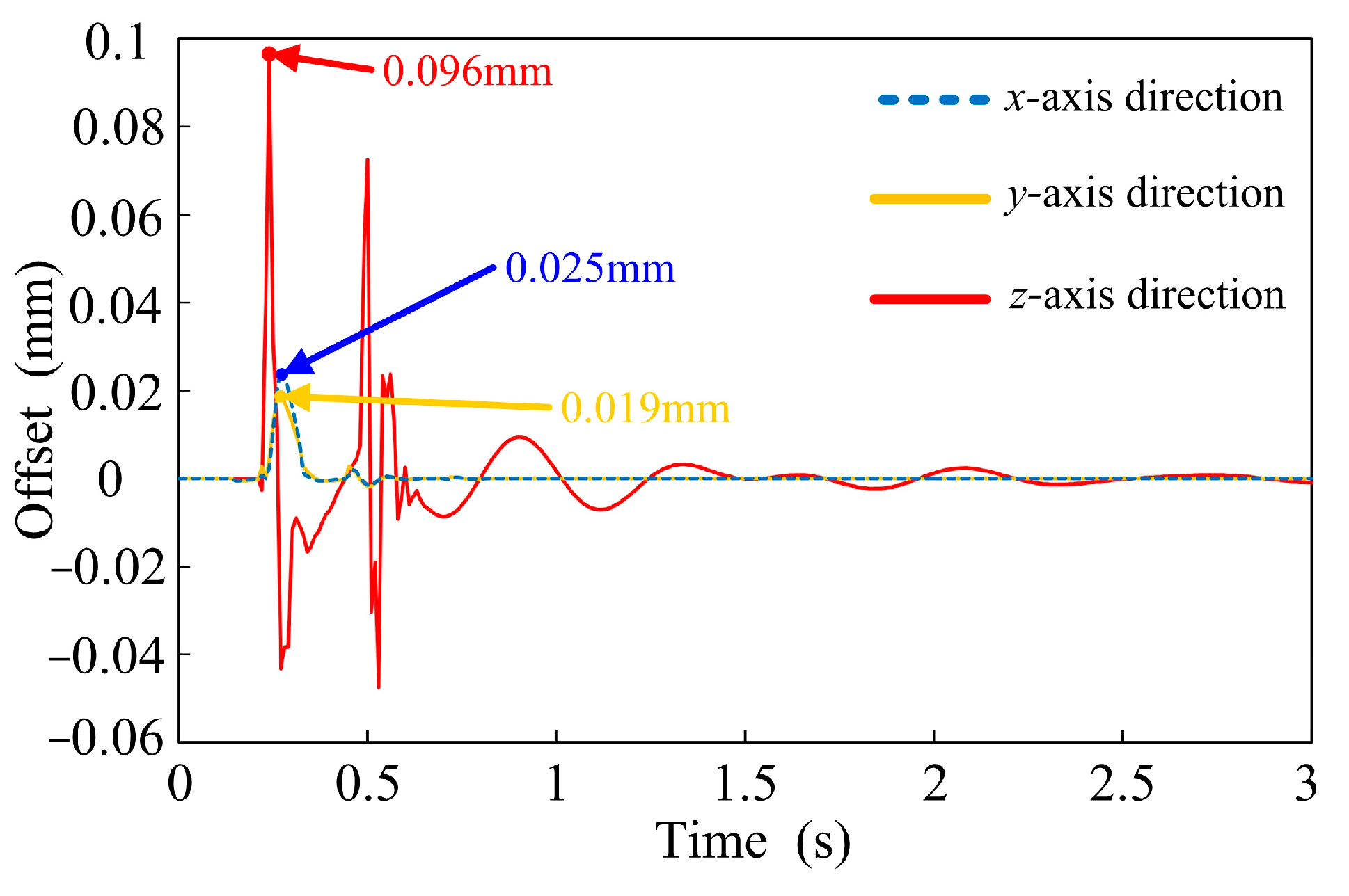
3.2. Contrastive Analysis of Radial and Axial Offsets

According to Section 2.5, the accelerations in Figure 5 were imported into ADAMS/View for dynamic response analysis of the flywheel. In order to eliminate the interference of the gyroscopic effect caused by the high-speed rotation of the flywheel and to further highlight the influence of pulse road excitation on the stability of the magnetic bearing–flywheel system, the rotational speed of the flywheel was set to 1000 r/min.

The dynamic response of the flywheel along the x-axis, y-axis, and z-axis under pulse road excitation is shown in Figure 6. The results show that under pulse road excitation, the axial offset of the flywheel was relatively large, with a peak of 0.096 mm, while the radial offset of the flywheel was much smaller than the axial offset, with a peak of only 0.025 mm, which can be ignored relative to the axial offset. Namely, under pulse road excitation, the axial degree of freedom of the flywheel was more easily affected than the radial degree of freedom. In addition, similar results were also observed under other working conditions.

Therefore, in order to ensure control accuracy under pulse road excitation, more attention needed to be paid to the axial model, while the radial model could only use conventional modeling. That is, the axial magnetic suspension force was modified according to Equation (3), while the radial magnetic suspension force used the static model. Therefore, when considering automobile suspension and pulse road excitation in the following passage, only the axial dynamic response was analyzed.

3.3. Contrastive Analysis of Different Vehicle Types

According to Section 2.4, due to different natural frequencies, saloon vehicles and off-road vehicles have significant differences in the stiffness of the automobile suspension, and the dynamic response of the flywheel is also affected. As shown in Figure 7, under pulse road excitation, when the stiffness values of the automobile suspension were 40 N/mm and 100 N/mm, respectively (the other operating parameters are the same as in Section 3.2, including the damping ratio, sprung mass, rotational speed, etc.), the dynamic response of the flywheel along the z-axis was obtained.

The results show that the rules of dynamic response were different under the influence of these two different stiffness values of automobile suspension. When the stiffness was 100 N/mm, the peak of axial offset was larger, which was 0.112 mm, while its adjustment time was shorter, only 1.8 s. This is because the higher stiffness of the automobile suspension increased the vertical acceleration of the vehicle and had a faster response speed, thus affecting the dynamic response of the flywheel. In addition, it is worth noting that when the stiffness of the automobile suspension was too low, the axial offset of the flywheel was quite large, with a peak of 0.218 mm, which easily collided with the auxiliary bearing. This is because the lower the stiffness of the automobile suspension, the larger the deformation of the automobile suspension. Therefore, it is necessary to avoid situations where the automobile suspension stiffness does not match the structure of the vehicle to prevent violent vibration.

Therefore, dynamic response analysis was conducted for the automobile suspension stiffness values of 40 N/mm and 100 N/mm in the following passage (without studying stiffness that is too low), and different control strategies and correction models are summarized based on the different rules of dynamic response.

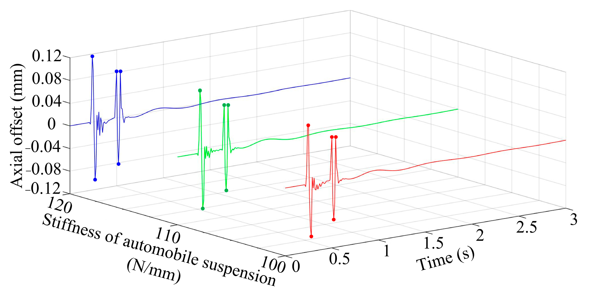
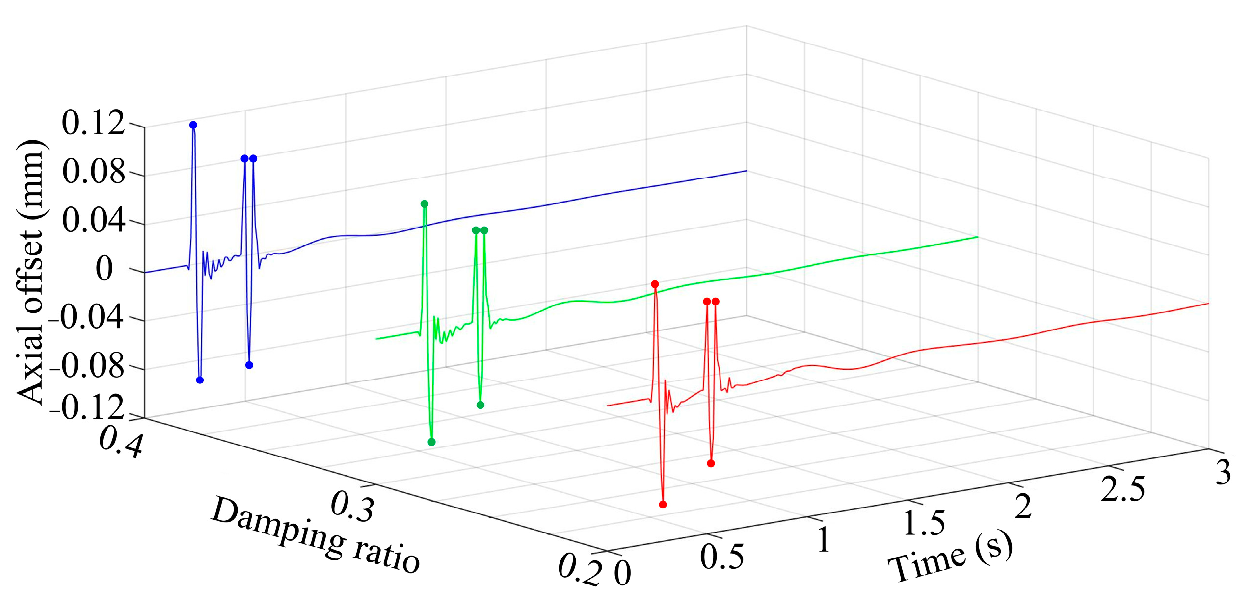
3.4. Different Stiffness Values of Automobile Suspension

Since the stiffness values of active automobile suspension are adjusted adaptively with the driving and road conditions, three different low automobile suspension stiffness values were selected according to Section 3.3: c₁ = 40 N/mm, c₂ = 45 N/mm, and c₃ = 50 N/mm (the other operating parameters are the same as in Section 3.2).

As shown in Figure 8, there was a dynamic response of the flywheel along the z-axis when the vehicle with low automobile suspension stiffness passed the speed bump. The results show that in a certain range of low automobile suspension stiffness, the trend of axial deviation was roughly the same. When the front wheel passed the speed bump, the flywheel went through a course of lead and lag with a large amplitude in the direction of the z-axis. When the rear wheel passed the speed bump, the flywheel went through a course of lead, lag, and lead with a smaller amplitude in the direction of the z-axis (among them, the second lead had a smaller amplitude). After that, the flywheel gradually returned to stability after a certain period of oscillation near the equilibrium position. Furthermore, with the increase in the stiffness of the automobile suspension, the axial offset of the flywheel increased slightly, while the adjustment time decreased obviously.

Since the axial deviations shown in Figure 8 had the same trends and the trends were regular, the main migration points of the flywheel were selected to correct for the Δz_f in Equation (3) by introducing weight factors:

$$∆z_f=k_f\cdot {\displaystyle {\int }_0^t{\displaystyle {\int }_0^{\xi }{a}_f(t)\mathrm{d}\xi \cdot \mathrm{dt}}}$$

(6)

where k_f is the weight factor; t is the simulation time; ξ is the intermediate of the integral; a_f(t) is the equation of the foundation acceleration with t.

Therefore, according to Figure 8, five groups of the main migration points were selected, with the stiffness of the automobile suspension as the independent variable. The Lagrange interpolation was used to estimate the axial offset, and the weight factor k_f was corrected.

Table 1. Offset proportions under different low automobile suspension stiffness values.

	c3/c2	c2/c1	c3/c1	OPi
Main migration point 1	1.08	1.08	1.17	1.11
Main migration point 2	1.31	1.27	1.65	1.41
Main migration point 3	1.14	1.06	1.21	1.14
Main migration point 4	1.25	1.30	1.62	1.39
Main migration point 5	1.30	1.32	1.72	1.45

shows the offset proportions (OPs) of the main migration points at low automobile suspension stiffness.

As shown in Table 1, mean fitting was carried out for the OPs under different low automobile suspension stiffness values, and the revised k_f1 was obtained:

$$k_{f1}=\frac{1}{N}\left({\displaystyle \sum _{i=1}^N\left[{\mathrm{OP}}_i\right]}\right)\approx 1.30$$

(7)

where k_f1 is the weight factor under different low automobile suspension stiffness values; N is the number of main migration points.

In order to further analyze the rule of axial deviation within a range of high automobile suspension stiffness under pulse road excitation, three different high automobile suspension stiffness values were selected: c₁ = 100 N/mm, c₂ = 110 N/mm, and c₃ = 120 N/mm (the other operating parameters were the same as in Section 3.2).

As shown in Figure 9, there was a dynamic response of the flywheel along the z-axis when the vehicle with high automobile suspension stiffness passed the speed bump. The results show that within a certain range of high automobile suspension stiffness, the trend of axial deviation was roughly the same. When the front wheel passed the speed bump, the flywheel went through a course of lead and lag with a large amplitude in the direction of the z-axis. When the rear wheel passed the speed bump, the flywheel went through a course of lead, lag, and lead with a smaller amplitude in the direction of the z-axis (among them, the second lead had a smaller amplitude). After that, the flywheel gradually returned to stability after a short oscillation near the equilibrium position. Furthermore, with the increase in the stiffness of automobile suspension, the axial offset of the flywheel tended to increase slightly, while the adjustment time was basically stable at 1.5 s.

Figure 9 shows that the axial deviations of the flywheel had the same trends and the trends were regular. Therefore, the stiffness of the automobile suspension was taken as the independent variable, and Lagrange interpolation was used to correct for the weight factor k_f.

Table 2. Offset proportions under high automobile suspension stiffness.

	c3/c2	c2/c1	c3/c1	OPi
Main migration point 1	1.06	1.05	1.11	1.07
Main migration point 2	1.05	1.05	1.11	1.07
Main migration point 3	1.04	1.01	1.05	1.03
Main migration point 4	1.12	1.06	1.19	1.12
Main migration point 5	1.07	1.04	1.11	1.07

shows the OPs of the main migration points at high automobile suspension stiffness values.

As shown in Table 2, mean fitting was carried out for the OPs under different high automobile suspension stiffness values, and the revised k_f2 was obtained:

$$k_{f2}=\frac{1}{N}\left({\displaystyle \sum _{i=1}^N\left[{\mathrm{OP}}_i\right]}\right)\approx 1.07$$

(8)

where k_f2 is the weight factor under different high automobile suspension stiffness values.

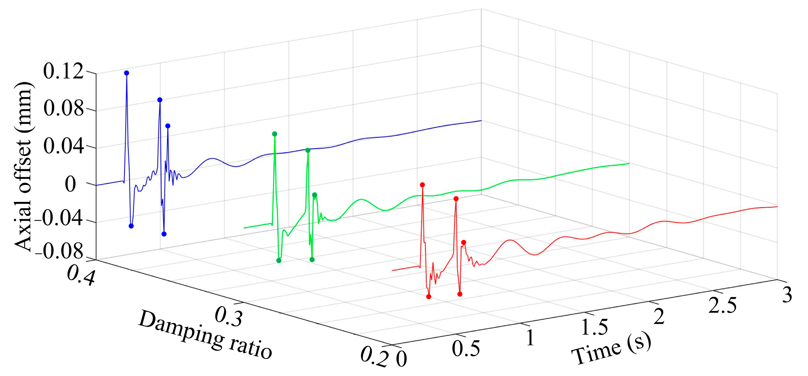
3.5. Different Damping Ratios

According to Section 3.4, under the pulse road excitation conditions, when the stiffness values of the automobile suspension were different, the dynamic response of the flywheel along the z-axis was different. Therefore, it was necessary to conduct dynamic response analysis under different damping ratios for two automobile suspension stiffness values (40 N/mm and 100 N/mm) so that different control strategies and correction models could be summarized according to the different rules of dynamic response.

The damping characteristics of the active automobile suspension were adjusted adaptively when the vehicle was operating. Therefore, three different damping ratios were taken (ψ₁ = 0.2, ψ₂ = 0.3, and ψ₃ = 0.4), and the stiffness value of the automobile suspension was c = 40 N/mm (the other operating parameters were the same as in Section 3.2).

Figure 10 shows the dynamic response of the flywheel along the z-axis under the pulse road excitation conditions when the damping ratio was different (c = 40 N/mm). The results show that within a certain range of damping ratios, the trend of axial deviation was roughly the same. When the front wheel passed the speed bump, the flywheel went through a course of lead and lag with a large amplitude in the direction of the z-axis. When the rear wheel passed the speed bump, the flywheel went through a course of lead, lag, and lead with a smaller amplitude in the direction of the z-axis (among them, the second lead had a smaller amplitude). After that, the flywheel gradually returned to stability after oscillating near the equilibrium position. Furthermore, with the increase in the damping ratios, the amplitudes of the first four main offset points increased slightly, while the amplitude of the fifth main offset point increased obviously. In addition, the adjustment time was significantly reduced.

The axial deviations of the flywheel shown in Figure 10 had the same trends and the trends were regular. Therefore, five groups of main migration points were selected, with the damping ratio as the independent variable. The Lagrange interpolation was used to correct for the weight factor k_f.

Table 3. Offset proportions under different damping ratios (c = 40 N/mm).

	c3/c2	c2/c1	c3/c1	OPi
Main migration point 1	1.18	1.11	1.31	1.20
Main migration point 2	1.19	1.24	1.48	1.30
Main migration point 3	1.12	1.10	1.23	1.15
Main migration point 4	1.39	1.18	1.64	1.40
Main migration point 5	2.10	1.44	3.02	2.19

shows the OPs of main migration points at different damping ratios (c = 40 N/mm).

As shown in Table 3, mean fitting was carried out for the OPs under different damping ratios, and the revised k_f3 was obtained:

$$k_{f3}=\frac{1}{N}\left({\displaystyle \sum _{i=1}^N\left[{\mathrm{OP}}_i\right]}\right)\approx 1.45$$

(9)

where k_f3 is the weight factor under different damping ratios (c = 40 N/mm).

In order to analyze the influence of different damping ratios on the rules of axial deviation under pulse road excitation when the stiffness of automobile suspension is high, three different damping ratios were selected (ψ₁ = 0.2, ψ₂ = 0.3, and ψ₃ = 0.4), while the stiffness of automobile suspension was 100N/mm (the other operating parameters were the same as in Section 3.2).

As shown in Figure 11, there was a dynamic response of the flywheel along the z-axis under the pulse road excitation conditions when the damping ratio was different (c = 100 N/mm). The results show that the trend of axial deviation was roughly the same. When the front wheel passed the speed bump, the flywheel went through a course of lead and lag with a large amplitude in the axial direction. When the rear wheel passed the speed bump, the flywheel went through a course of lead, lag, and lead with a smaller amplitude in the axial direction. After that, the flywheel gradually returned to stability after a short oscillation near the equilibrium position. Furthermore, with the increase in the damping ratios, the axial offset of the flywheel increased slightly, while the adjustment time decreased slightly.

Figure 11 shows that the axial deviations of the flywheel had the same trends and the trends were regular. Therefore, the damping ratio was taken as the independent variable, and Lagrange interpolation was used to correct for the weight factor k_f.

Table 4. Offset proportions under different damping ratios (c = 100 N/mm).

	c3/c2	c2/c1	c3/c1	OPi
Main migration point 1	1.11	1.16	1.29	1.19
Main migration point 2	1.04	1.04	1.08	1.05
Main migration point 3	1.05	1.05	1.10	1.07
Main migration point 4	1.31	1.10	1.44	1.28
Main migration point 5	1.08	1.07	1.15	1.10

shows the OPs of the main migration points at different damping ratios (c = 100 N/mm).

As shown in Table 4, mean fitting was carried out for the OPs under different damping ratios, and the revised k_f4 was obtained:

$$k_{f4}=\frac{1}{N}\left({\displaystyle \sum _{i=1}^N\left[{\mathrm{OP}}_i\right]}\right)\approx 1.14$$

(10)

where k_f4 is the weight factor under different damping ratios (c = 100 N/mm).

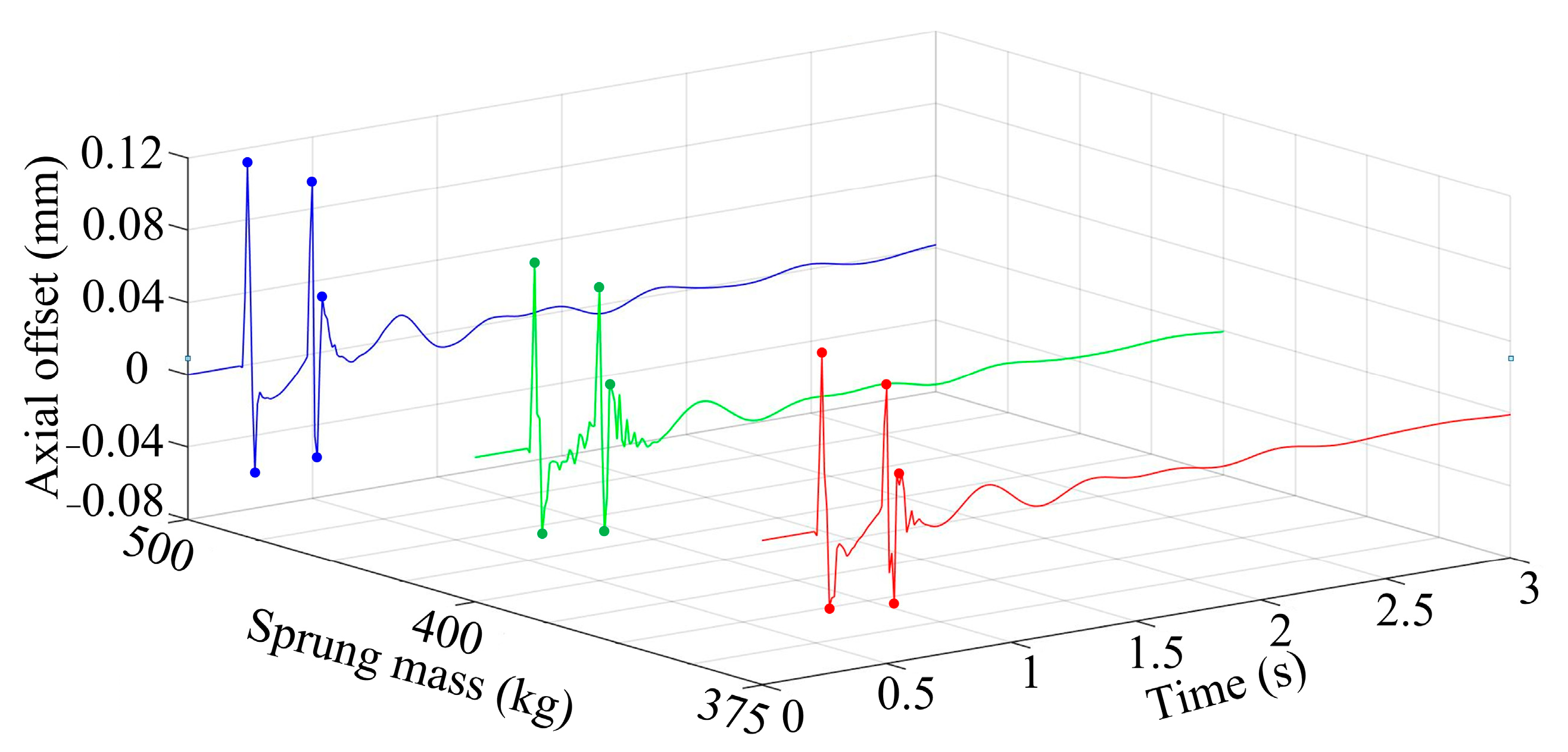
3.6. Different Sprung Masses

According to Equations (4) and (5), when the vehicle is operating, the sprung mass will affect the parameters of the automobile suspension, thus affecting the dynamic response of the flywheel. Therefore, different sprung masses were selected to analyze the rules of axial deviation within a certain range of sprung mass, and a corresponding correction model was developed. In addition, the dynamic response under two stiffness values of automobile suspension (40 N/mm and 100 N/mm) was analyzed.

Three different sprung masses were selected (m_s1 = 375 kg, m_s2 = 400 kg, and m_s3 = 500 kg), which correspond to no load, light load, and full load, respectively. Furthermore, the stiffness of the automobile suspension was c = 40 N/mm (the other operating parameters were the same as in Section 3.2).

Figure 12 shows the dynamic response of the flywheel along the z-axis under the pulse road excitation conditions when the sprung mass was different (c = 40 N/mm). The results show that within a certain range of sprung masses, the trend of axial deviation was roughly the same. When the front wheel passed the speed bump, the flywheel went through a course of lead and lag with a large amplitude in the axial direction. When the rear wheel passed the speed bump, the flywheel went through a course of lead, lag, and lead with a smaller amplitude in the axial direction. After that, the flywheel gradually returned to stability after a certain period of oscillation near the equilibrium position. Furthermore, with the increases in the sprung masses, the axial offset and adjustment time increased slightly.

Since the axial deviations of the flywheel, shown in Figure 12, had the same trends and the trend were regular, five groups of main migration points in Figure 12 were selected as the independent variables, and Lagrange interpolation was used to correct for the weight factor k_f.

Table 5. Offset proportions under different sprung masses (c = 40 N/mm).

	c3/c2	c2/c1	c3/c1	OPi
Main migration point 1	1.10	1.04	1.15	1.10
Main migration point 2	1.24	1.13	1.40	1.26
Main migration point 3	1.17	1.12	1.30	1.20
Main migration point 4	1.11	1.10	1.23	1.15
Main migration point 5	1.14	1.13	1.30	1.19

shows the OPs of the main migration points at different sprung masses (c = 40 N/mm).

As shown in Table 5, mean fitting was carried out for OPs under different sprung masses, and the revised k_f5 was obtained:

$$k_{f5}=\frac{1}{N}\left({\displaystyle \sum _{i=1}^N\left[{\mathrm{OP}}_i\right]}\right)\approx 1.18$$

(11)

where k_f5 is the weight factor under different sprung masses (c = 40 N/mm).

In addition, in order to analyze the influence of different sprung masses on the rules of axial deviation under pulse road excitation when the stiffness of the automobile suspension is high, three different sprung masses were selected: m_s1 = 375 kg, m_s2 = 400 kg, and m_s3 = 500 kg (the other operating parameters were the same as in Section 3.2).

As shown in Figure 13, there was a dynamic response of the flywheel along the z-axis under the pulse road excitation conditions when the sprung mass was different (c = 100 N/mm). The results show that under different sprung masses, the trend of deviation was roughly the same. When the front wheel passed the speed bump, the flywheel went through a course of lead and lag with a large amplitude in the direction of the z-axis. When the rear wheel passed the speed bump, the flywheel went through a course of lead, lag, and lead with a small amplitude in the direction of the z-axis. After that, the flywheel gradually returned to stability after a short oscillation near the equilibrium position. Furthermore, with the increases in the sprung masses, the axial offset of the flywheel increased slightly, and the adjustment time was basically stable at 1.5 s.

Figure 13 shows that the axial deviations of the flywheel had the same trends and the trends were regular. Therefore, the sprung mass was taken as the independent variable, and Lagrange interpolation was used to correct for the weight factor k_f.

Table 6. Offset proportions under different sprung masses (c = 100 N/mm).

	c3/c2	c2/c1	c3/c1	OPi
Main migration point 1	1.11	1.06	1.18	1.12
Main migration point 2	1.12	1.06	1.18	1.12
Main migration point 3	1.18	1.07	1.26	1.17
Main migration point 4	1.17	1.11	1.30	1.19
Main migration point 5	1.09	1.05	1.15	1.10

shows the OPs of the main migration points at different sprung masses (c = 100 N/mm).

As shown in Table 6, mean fitting was carried out for the OPs under different sprung masses, and the revised k_f6 was obtained:

$$k_{f6}=\frac{1}{N}\left({\displaystyle \sum _{i=1}^N\left[{\mathrm{OP}}_i\right]}\right)\approx 1.14$$

(12)

where k_f6 is the weight factor under different sprung masses (c = 100 N/mm).

Therefore, according to Equations (7)–(12), the weight factors of different parameters of automobile suspension are summarized in

Table 7. Weight factors of different automobile suspension parameters under pulse road excitation.

	Different Stiffness Values of Automobile Suspension	Different Damping Ratios	Different Sprung Masses
Low stiffness of automobile suspension	kf1	kf3	kf5
High stiffness of automobile suspension	kf2	kf4	kf6

under pulse road excitation.

Therefore, combining Table 7 and Equations (3) and (6), the correction model of axial magnetic suspension force considering automobile suspension and pulse road excitation can be summarized as follows:

$$F_{dz}=k_{dz}\cdot z+k_{diz}\cdot i_{z0}=\left|\frac{z-z_0}{k_{fp}\cdot {\displaystyle {\int }_0^t{\displaystyle {\int }_0^{\xi }{a}_f(t)\mathrm{d}\xi \cdot \mathrm{dt}}}}\right|k_z\cdot z+\left(1+\frac{∆i_{fz}}{i_{z0}}\right)\cdot i_{z0}$$

(13)

where k_fp is the weight factor based on automobile suspension and pulse road excitation, with values based on Table 7, which depends on different automobile suspension values.

It is worth noting that in the common ranges of the stiffness of automobile suspension, damping ratios, and sprung masses, the weight factor can be modified by equidistant interpolation, and thus, the accuracy of the magnetic suspension force under pulse road excitation can be improved. That is to say, the correction is not limited to the above parameters of automobile suspension. Multiple equidistant interpolations can be performed in the common range, and the offset of the flywheel under other parameters of the automobile suspension can be estimated.

3.7. Brief Summary of Bullet Points

Based on the above, the magnetic suspension force model can be corrected by considering the influence of automobile suspension and typical road conditions. Thus, a brief summary of the modeling method is provided:

(1)

In order to improve the calculation accuracy of the dynamic magnetic suspension force model, a dynamic model considering automobile suspension and typical road conditions should be established based on ADAMS, so as to correct the magnetic suspension force model according to the dynamic response rules.

(2)

It is worth noting that under the typical road conditions (speed bump) used in this paper, the radial degree of freedom was particularly less affected compared to the axial degree of freedom. Therefore, only the axial magnetic suspension force model was taken as an example for model correction in this paper. In addition, a stiffness value of automobile suspension that is too small can cause excessive vibration of the vehicle body, which is avoided during the vehicle manufacturing process. Therefore, such parameters of automobile suspension can be disregarded during modeling.

(3)

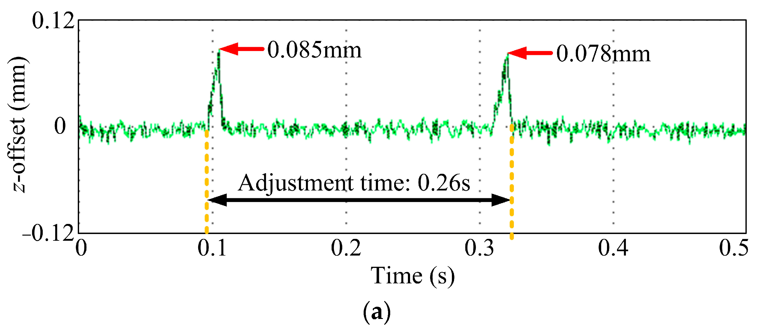
Under the comprehensive consideration of automobile suspension and typical road conditions, it can be found that the main factor affecting the dynamic response rules is the vehicle type. Compared to the dynamic response using saloon vehicles, the dynamic response using off-road vehicles has a shorter adjustment time, but the overall offset also significantly increases. Furthermore, for the dynamic response using saloon vehicles, a small change in the automobile suspension stiffness will significantly affect the adjustment time. However, when the vehicle type is the same, within a certain range of automobile suspension parameters, the dynamic response rules of the flywheel do not change significantly; it is mainly a small change in the overall offset.

(4)

For cases such as in this paper, where the dynamic response had the same trend and the trend was regular within a certain range of independent variables, the Lagrange interpolation method can be used for mean fitting to correct the magnetic suspension force model.

3.8. PID Control Diagram

A PID control diagram based on pulse road excitation is shown in Figure 14. Double closed-loop feedback control of the inner current loop and the outer displacement loop was adopted in the system. Furthermore, the magnetic suspension control system was composed of radial control and axial control: the PID controller, radial static model, and hysteresis comparator were in the radial control module; the PID controller, model selection module, axial correction model, and compensation current module were in the axial module. Moreover, before entering the correction model, model selection was carried out according to the changes in the parameters of automobile suspension so as to select the appropriate weight factor according to Table 7. In addition, a flywheel battery model, displacement sensors, and a foundation offset correction module are also included in the control diagram.

It is worth noting that the stiffness of the magnetic suspension model was corrected by the correction model proposed in this study, which comprehensively considers automobile suspension and pulse road excitation. Therefore, when the influence of automobile suspension and pulse road excitation is considered, the model results can be corrected more accurately by dynamically calculating the foundation offset.

3.9. PID Controller Applicable to Different Vehicle Types

According to Section 3.3, for saloon and off-road vehicles, due to different parameters of the automobile suspension, the rules of dynamic response were also different under the pulse road excitation conditions. Therefore, a PID control strategy applicable to different vehicle types was further selected.

For sedan vehicles with low automobile suspension stiffness, since the adjustment time was relatively longer under the pulse road excitation conditions, an incomplete differential PID could be selected. Due to the addition of an inertial link, the differential action time becomes longer, which is beneficial for suppressing noise and improving the speed of response. Its transfer function is as follows:

$$G_c=K_p+\frac{K_i}{s}+\frac{K_d\cdot s}{1+T_d\cdot s}$$

(14)

where K_p, K_i, and K_d are the proportional, integral, and differential coefficients of the incomplete differential PID, respectively; T_d is the differential time constant.

For off-road vehicles with high automobile suspension stiffness, since the overshoot of the axial offset was relatively larger under the pulse road excitation conditions, a differential advanced PID could be selected. Because the controlled parameters and their rates of change were added to the output signal of the differential link and input into the PI controller, the overshoot was effectively reduced. Its transfer function is as follows:

$$G_c=K_p+\frac{K_i}{s}+\frac{1+T_d\cdot s}{1+\gamma T_d\cdot s}$$

(15)

where K_p, K_i, and K_d are the proportional, integral, and differential coefficients of the differential advanced PID, respectively; T_d is the differential time constant; γ is the filtering coefficient.

4. Experiment and Analysis

Due to the complexity of disturbances under vehicle-mounted conditions, the dynamic performance of a flywheel battery will be inevitably affected. Therefore, in order to make the obtained experimental data closer to real operating conditions, it was necessary to build an experimental platform based on pulse road excitation.

4.1. Experimental Platform for Pulse Road Excitation

As shown in Figure 15, the overall experimental platform for pulse road excitation was composed of a flywheel battery with a virtual inertia spindle, an electric vehicle, a speed bump, and a control system platform. The flywheel battery was installed on the electric vehicle to imitate the vehicle-mounted conditions.

To facilitate testing, the control system platform was placed on a trailer, which was connected to an electric vehicle through a connector. The connector provided a buffering effect for the electric vehicle when passing the speed bump, avoiding adverse effects on the experimental results due to the inertia impact of the trailer on the electric vehicle. The control system platform was mainly composed of a power supply, an oscilloscope, a magnetic suspension control system (its control diagram is shown in Figure 14), a user interface, etc. Among them, a DSP board, a displacement interface circuit board, a power drive circuit board, and displacement sensors were included in the hardware of the control system. In addition, in order to prevent the impact of electromagnetic interference on the circuit, an RC filtering circuit was set. Furthermore, the software filtering was also set in the program to ensure sampling accuracy. It is worth noting that, as shown in Figure 15, the real-time interactive interface based on LABVIEW can timely reflect the operation situation of the flywheel battery located on the electric vehicle, and the magnetic bearing–flywheel system can be controlled by PID through the interface.

4.2. Performance Tests

In order to verify whether the corrected model considering automobile suspension and pulse road excitation had better anti-interference capability than the static model, performance tests were conducted based on the experimental platform shown in Figure 15. The experimental process was as follows: First, the motor was driven to maintain the flywheel at a constant rotating speed of 1000 r/min (in order to eliminate the interference of the gyroscopic effect caused by high-speed rotation and highlight the influence of pulse road excitation), and then the electric vehicle passed the speed bump twice at a uniform speed of 10 km/h. Two different magnetic suspension force models were used, namely a static model and a dynamic correction model. In addition, the parameters of the speed bump were 980 mm in length, 340 mm in width, and 40 mm in height. The wheelbase of the vehicle was 500 mm.

As shown in Figure 16a, there was a displacement waveform of the flywheel along the z-axis when using the static model for magnetic suspension force. It can be observed that under the influence of automobile suspension and pulse road excitation, as the front and rear wheels of the electric vehicle passed the speed bump, respectively, the flywheel underwent two lead offsets in the axial direction, with values of 0.085 mm and 0.078 mm. Then, under the action of the magnetic suspension control system, the flywheel quickly returned to the equilibrium position, with an adjustment time of 0.26 s. Furthermore, when the dynamic correction model was used for the magnetic suspension force, as shown in Figure 16b, it was found that the trend of its dynamic response was basically the same as the dynamic response using the static model, but it had more advantages in leading the offset and adjustment time. As the front and rear wheels of the electric vehicle passed the speed bump, respectively, the two leading offsets were 0.074 mm and 0.070 mm, respectively, and the adjustment time was 0.24 s. Therefore, it can be seen that using the dynamic correction model proposed in this paper ensured the stable suspension of the flywheel under the conditions of a speed bump. Furthermore, compared to the static model, the dynamic correction model had better anti-interference capability.

It should be noted that due to the difference in the parameters between the experimental vehicle and the actual vehicle (especially the sprung mass), the course of lag was not obvious when the flywheel returned to the equilibrium position after being disturbed. However, when reaching the highest point of the speed bump, the trend of the dynamic response was roughly the same as the results of the simulation, as shown in Figure 6.

5. Conclusions

In this study, taking a vehicle-mounted flywheel battery with a virtual inertia spindle as an example, the dynamic performance of a magnetic bearing–flywheel system was analyzed by combining the influence of the automobile suspension and pulse road excitation. Furthermore, according to the rules of dynamic response under different parameters of automobile suspension, a correction model of the magnetic suspension force was proposed and different PID control strategies were summarized. Finally, performance tests were carried out. The experimental results prove that the correction model has good anti-interference performance.

Furthermore, this paper studied speed bumps as road conditions, which are typical pulse excitation conditions. In order to make the model more comprehensive, more road conditions should be further considered. Therefore, dynamic response analysis of a magnetic bearing–flywheel system should be carried out regarding continuous random excitation or special road conditions (such as frontal collision, etc.) in the future to further improve the applicability of the model.

In addition, it is worth noting that in order to highlight the advantages of accurate mathematical models, this paper only used the classic PID control strategy to achieve stable suspension of the flywheel. However, a suitable control strategy is also an important means to improve system stability. Since the research object of this paper was a vehicle-mounted flywheel battery, the control strategies used to improve vehicle stability are also of great significance to the construction of a magnetic suspension control system. Including the comprehensive chassis control strategy of FWIC-EV based on sliding-mode control, the dynamics integrated control for four-wheel independent-control electric vehicles, etc., which can even improve the system’s stability under extreme conditions. Therefore, in the future, certain application research will be conducted on these kinds of control strategies.

References

1. Ren, Y.; Su, D.; Fang, J.C. Whirling modes stability criterion for a magnetically suspended flywheel rotor with significant gyroscopic effects and bending modes. IEEE Trans. Power Electron. 2013, 28, 5890–5901. [Google Scholar] [CrossRef]
2. Li, X.J.; Anvari, B.; Palazzolo, A.; Wang, Z.Y.; Toliyat, H. A utility-scale flywheel energy storage system with a shaftless, hubless, high-strength steel rotor. IEEE Trans. Ind. Electron. 2018, 65, 6667–6675. [Google Scholar] [CrossRef]
3. Peng, C.; Zheng, S.Q.; Huang, Z.Y.; Zhou, X.X. Complete synchronous vibration suppression for a variable-speed magnetically suspended flywheel using phase lead compensation. IEEE Trans. Ind. Electron. 2018, 65, 5837–5846. [Google Scholar] [CrossRef]
4. Sun, B.; Dragičević, T.; Freijedo, F.D.; Vasquez, J.C.; Guerrero, J.M. A control algorithm for electric vehicle fast charging stations equipped with flywheel energy storage systems. IEEE Trans. Power Electron. 2016, 31, 6674–6685. [Google Scholar] [CrossRef]
5. Sun, Y.G.; Xu, J.Q.; Han, W.; Lin, G.B.; Mumtaz, S. Deep learning based semi-supervised control for vertical security of maglev vehicle with guaranteed bounded airgap. IEEE Trans. Intell. Transp. Syst. 2021, 22, 4431–4442. [Google Scholar] [CrossRef]
6. Glücker, P.; Kivekäs, K.; Vepsäläinen, J.; Mouratidis, P.; Schneider, M.; Rinderknecht, S.; Tammi, K. Prolongation of Battery Lifetime for Electric Buses through Flywheel Integration. Energies 2021, 14, 899. [Google Scholar] [CrossRef]
7. Peng, C.; Zhu, M.T.; Wang, K.; Ren, Y.; Deng, Z.Q. A two-stage synchronous vibration control for magnetically suspended rotor system in the full speed range. IEEE Trans. Ind. Electron. 2020, 67, 480–489. [Google Scholar] [CrossRef]
8. Han, B.C.; Chen, Y.L.; Zheng, S.Q.; Li, M.X.; Xie, J.J. Whirl mode suppression for AMB-rotor systems in control moment gyros considering significant gyroscopic effects. IEEE Trans. Ind. Electron. 2020, 68, 4249–4258. [Google Scholar] [CrossRef]
9. Ren, Y.; Chen, X.C.; Cai, Y.W.; Zhang, H.J.; Xin, C.J.; Lin, Q. Attitude-rate measurement and control integration using magnetically suspended control and sensitive gyroscopes. IEEE Trans. Ind. Electron. 2018, 65, 4921–4932. [Google Scholar] [CrossRef]
10. Zhang, W.Y.; Gu, X.W.; Zhang, L.D. Robust Controller Considering Road Disturbances for a Vehicular Flywheel Battery System. Energies 2022, 15, 5432. [Google Scholar] [CrossRef]
11. Zhang, W.Y.; Yang, H.K.; Cheng, L.; Zhu, H.Q. Modeling Based on Exact Segmentation of Magnetic Field for a Centripetal Force Type-Magnetic Bearing. IEEE Trans. Ind. Electron. 2020, 67, 7691–7701. [Google Scholar] [CrossRef]
12. Zhang, W.Y.; Cheng, L.; Zhu, H.Q. Suspension Force Error Source Analysis and Multidimensional Dynamic Model for a Centripetal Force Type-Magnetic Bearing. IEEE Trans. Ind. Electron. 2020, 67, 7617–7628. [Google Scholar] [CrossRef]
13. Zhang, W.Y.; Zhang, L.D.; Li, K.; Zhu, H.Q. Dynamic correction model considering influence of foundation motions for a centripetal force type-magnetic bearing. IEEE Trans. Ind. Electron. 2021, 68, 9811–9821. [Google Scholar] [CrossRef]
14. Zhang, P.; Zhu, C. Vibration Control of Base-Excited Rotors Supported by Active Magnetic Bearing Using a Model-Based Compensation Method. IEEE Trans. Ind. Electron. 2023. [Google Scholar] [CrossRef]
15. Ding, G.P.; Zhou, Z.D.; Hu, Y.F. Test of base vibration influence on dynamics of a magnetic suspended disk. In Proceedings of the 2008 IEEE/ASME International Conference on Advanced Intelligent Mechatronics, Xi’an, China, 2–5 July 2008; pp. 308–313. [Google Scholar]
16. Soni, T.; Sodhi, R. Impact of harmonic road disturbances on active magnetic bearing supported flywheel energy storage system in electric vehicles. In Proceedings of the 2019 IEEE Transportation Electrification Conference (ITEC-India), Bengaluru, India, 17–19 December 2019; pp. 1–4. [Google Scholar]
17. Kasarda, M.E.; Clements, J.; Wicks, A.L.; Hall, C.D.; Kirk, R.G. Effect of sinusoidal base motion on a magnetic bearing. In Proceedings of the 2000 IEEE International Conference on Control Applications, Anchorage, AK, USA, 27 September 2000; pp. 144–149. [Google Scholar]
18. Zhang, W.Y.; Wang, J.P.; Zhu, P.F.; Yu, J.X. A novel vehicle-mounted magnetic suspension flywheel battery with a virtual inertia spindle. IEEE Trans. Ind. Electron. 2022, 69, 5973–5983. [Google Scholar] [CrossRef]
19. Preumont, A.; Seto, K. Active Control of Structures; John Wiley & Sons: New York, NY, USA, 2008. [Google Scholar]
20. Suciu, C.V.; Tobiishi, T.; Mouri, R. Modeling and Simulation of a Vehicle Suspension with Variable Damping and Elastic Properties versus the Excitation Frequency. In Proceedings of the 2011 International Conference on P2P, Parallel, Grid, Cloud and Internet Computing, Barcelona, Spain, 26–28 October 2011; pp. 402–407. [Google Scholar]
Figure 1. Overall structure and magnetic circuits of the flywheel battery with a virtual inertia spindle. (1) Flywheel; (2) combined magnetic bearing; (3) radial magnetic bearing; (4) axial magnetic bearing; (5) housing; (6) motor; (7) radial bias flux; (8) radial control flux; (9) axial bias flux; (10) axial control flux.
Energies 16 04288 g001
Figure 2. Eccentricity diagram of flywheel.
Energies 16 04288 g002
Figure 3. Simulation model of vehicle in ADAMS/Car.
Energies 16 04288 g003
Figure 4. Magnetic bearing–flywheel system in ADAMS/View. (1) Combined magnetic bearing; (2) flywheel; (3) housing; (4) support base; (5) equivalent module of axial magnetic bearing; (6) equivalent module of radial magnetic bearing.
Energies 16 04288 g004
Figure 5. Acceleration of vehicle chassis under pulse road excitation. (a) The acceleration along the x-axis. (b) The acceleration along the y-axis. (c) The acceleration along the z-axis.
Energies 16 04288 g005
Figure 6. Dynamic response of flywheel under the pulse road excitation.
Energies 16 04288 g006
Figure 7. Dynamic response of flywheel under pulse road excitation.
Energies 16 04288 g007
Figure 8. Dynamic response of flywheel under low automobile suspension stiffness.
Energies 16 04288 g008
Figure 9. Dynamic response of flywheel under high automobile suspension stiffness.
Energies 16 04288 g009
Figure 10. Dynamic response of flywheel under different damping ratios (c = 40 N/mm).
Energies 16 04288 g010
Figure 11. Dynamic response of flywheel under different damping ratios (c = 100N/mm).
Energies 16 04288 g011
Figure 12. Dynamic response of flywheel under different sprung masses (c = 40 N/mm).
Energies 16 04288 g012
Figure 13. Dynamic response of flywheel under different sprung masses (c = 100 N/mm).
Energies 16 04288 g013
Figure 14. PID correction control diagram based on pulse road excitation.
Energies 16 04288 g014
Figure 15. The overall experimental platform of pulse road excitation.
Energies 16 04288 g015
Figure 16. The offsets of the flywheel under pulse road excitation. (a) The offset of the flywheel in the z-direction (static model). (b) The offset of the flywheel in the z-direction (correction model).
Energies 16 04288 g016aEnergies 16 04288 g016b