Benefit Evaluation of Carbon Reduction in Power Transmission and Transformation Projects Based on the Modified TOPSIS-RSR Method

Abstract

In order to fully achieve energy saving goals, it is necessary to establish a comprehensive evaluation system for carbon reduction in transmission and transformation projects. Subsequently, weights were assigned to these indicators using a combination of the fuzzy analytical hierarchy process (FAHP) and the entropy weight method (EWM) through both subjective and objective methods. Finally, the ultimate weights were obtained by applying the principle of minimum information. During the construction of the evaluation model, the rank–sum ratio (RSR) method was introduced into the Technique for Order Preference by Similarity to Ideal Solution (TOPSIS) for approximating ideal solution ranking. And the Euclidean distance in TOPSIS was replaced with standardized Euclidean distance, effectively avoiding evaluation discrepancies caused by different dimensions. The modified TOPSIS-RSR method was utilized to evaluate and rank power transmission and transformation projects in four regions. By comparing the test values of the two models, the superiority of the enhanced model was confirmed. Furthermore, the GM (1,1) model is used to predict the electricity sales volume of the optimal ranking area. This evaluation model can also be applied to the benefit evaluation of carbon reduction benefits in power transmission and transformation projects in other regions.

1. Introduction

Energy is the basis and driving force behind the economic development of modern society [1]. All sectors depend on energy supply to support their productive activities and service delivery. However, energy shortage has become a major problem in society [2]. With the continuous growth in the global demand for electricity and the restructuring of energy sources, the share of the power sector in energy consumption has become particularly important [3]. Through structural adjustment in the power industry over the past few decades, the proportion of non-fossil energy power generation and the proportion of power generation by high-efficiency thermal power units have increased [4,5], and carbon dioxide emissions has declined significantly [6,7]. According to relevant statistics, from 2006 to 2018, the reduction in carbon dioxide emissions in the Chinese electricity industry amounted to 13.7 billion tons [8], effectively slowing down the growth rate of total carbon dioxide emissions from electricity generation [9,10,11]. However, due to the large capital investment and high complexity of transmission and transformation projects [12], there is currently no clear standard evaluation system for the comprehensive benefits brought about by carbon reduction in these projects. Therefore, it is necessary to conduct a reasonable and comprehensive evaluation of them. Analyzing and evaluating the economic benefits, carbon reduction benefits, and social benefits of projects can effectively enhance the scientific nature of decision making.

Multi-criteria decision analysis (MCDA) is a decision-making method that comprehensively considers the multiple attributes of a problem to arrive at an optimal solution or best plan. MCDA is suitable for decision support in scenarios involving conflicting objectives across economic, environmental, social, and technological domains. Leveraging this advantage, the method has been applied across various research fields. Depending on the preferences of the decision maker, existing MCDA approaches have different paradigms for evaluating decision alternatives. Typically, these methods can be divided into two categories. Subjective methods that involve pairwise comparisons; these are objective methods that rely on the data themselves to rank decisions.

Currently, there are many commonly used subjective methods, including the following:

(a)

The analytic hierarchy process (AHP): This method constructs a hierarchical framework for problem evaluation and assesses the relative significance of various criteria through pairwise comparisons. Among the scholars who use this method, Chen Yunfeng [13] conducted a comprehensive evaluation of transmission and transformation projects based on specific criteria such as preliminary decision making, an implementation process, construction implementation, and sustainable development using the AHP method. However, due to the sole reliance on subjective evaluation methods, there is an issue of insufficient persuasiveness in the evaluation results.

(b)

The fuzzy analytic hierarchy process (FAHP): This method represents an adaptation of the AHP, employing fuzzy logic to manage uncertainties and ambiguities inherent in the decision-making process. Xu Dan [14] and Gao Chao [15] utilized the FAHP to construct a social benefit evaluation model for grid engineering projects. They validated this model, and compared to the AHP, the FAHP introduces fuzziness to subjective judgments, enhancing its comprehensiveness and adaptability. However, since this method still falls under subjective evaluation, it cannot guarantee the scientific validity of indicator selection.

(c)

Elimination and choice expressing reality (ELECTRE): This method requires experts to establish thresholds for consistency and inconsistency among different options, ranking them according to these criteria. Given that these thresholds often derive from expert experience and intuition, the method is highly subjective. Akram, M [16] extended the ELECTRE I methodology to accommodate group decision scenarios by utilizing Pythagorean fuzzy numbers (PFNs) as attributes for each criterion, thus creating the Pythagorean Fuzzy ELECTRE I (PF-ELECTRE I) method. The integration of PFNs improves the model’s capacity to manage fuzziness and incompleteness. The efficacy of this model was demonstrated through two environmental management case studies. Although both PF-ELECTRE I and the Fuzzy AHP (FAHP) methodologies embrace fuzziness, PF-ELECTRE I is more apt for contexts characterized by conflicts, while FAHP’s simpler calculations make it more widely acceptable.

In contrast to subjective methods, objective methods provide a systematic and transparent mechanism for weight distribution, which diminishes the influence of personal biases and subjective evaluations in the decision-making process. The common objective methods are as follows:

(a)

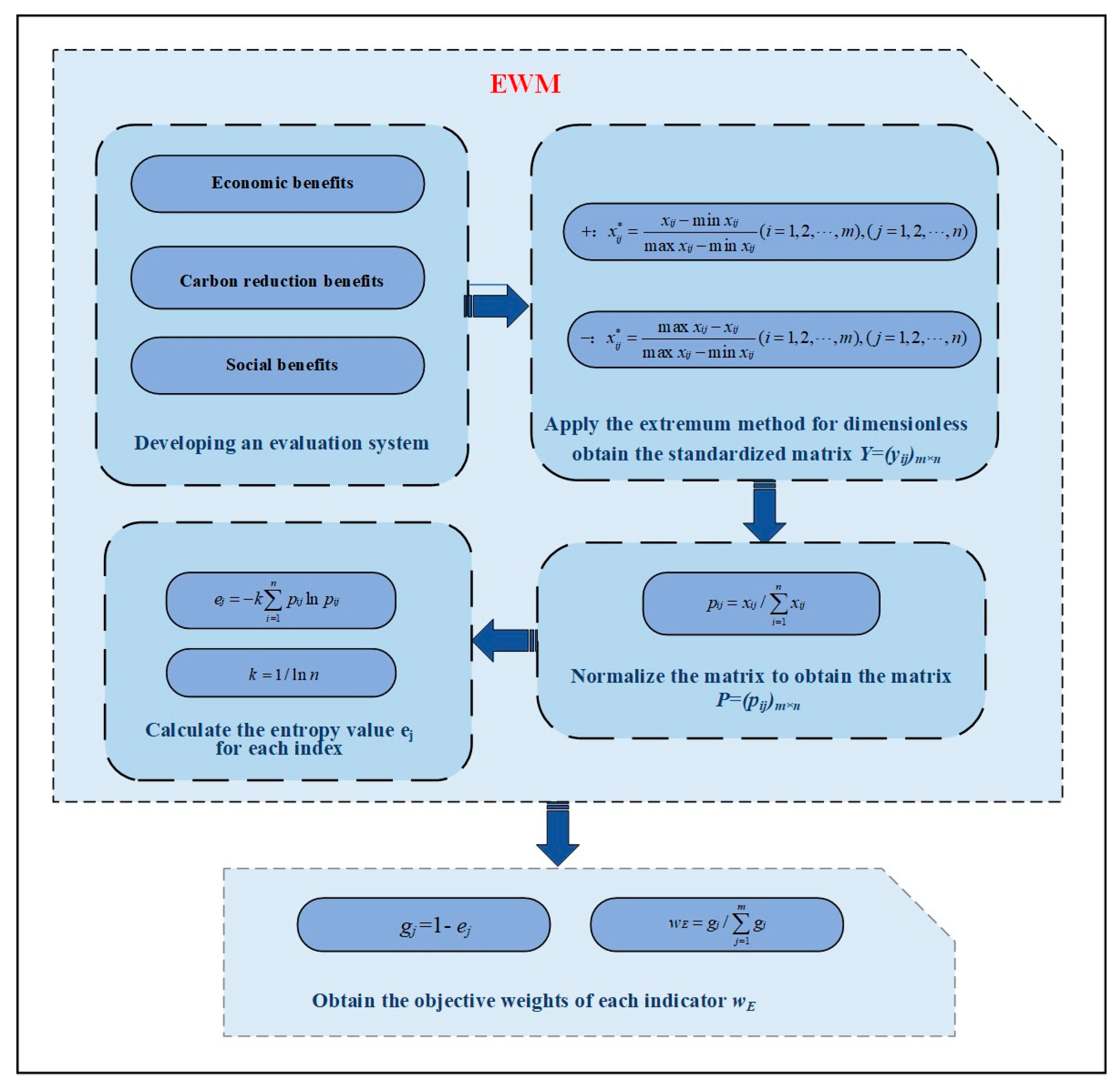
The entropy weight method (EWM): This method employs the concept of information entropy for determining the weights of different indicators. Information entropy quantifies the degree of dispersion among criteria. Criteria with higher dispersion levels contain more information and are consequently allocated greater weights. As this method is independent of external subjective evaluations, it is broadly applicable to scenarios that demand objective assessments and decisions. Its inherent flexibility also facilitates its integration with other decision-making frameworks, including the AHP and the Technique for Order of Preference by Similarity to Ideal Solution (TOPSIS). Many scholars like MRZ Banadkouki [17], Sijia Liu [18], and Minggao Chen [19] have utilized the EWM for calculating the weights of project indicators.

(b)

Technique for Order of Preference by Similarity to Ideal Solution (TOPSIS): This method orders the alternatives by computing their distances to both the optimal ideal point and the least favorable nadir point, based on the evaluation criteria. While the TOPSIS method often relies on subjective techniques to ascertain weights, it can also integrate objective approaches for setting criteria weights, or employ a hybrid weighting system. Wang, Y [20] improved the TOPSIS method by constructing positive and negative ideal solutions. However, in the comprehensive evaluation of projects, this method alone is relatively singular and cannot consider the comprehensiveness of indicators. Gebrehiwet [21] proposed a method to assess the risk of delays in the entire lifecycle of transmission and transformation projects. They constructed a comprehensive model based on TOPSIS and FAHP sequential preference techniques. By establishing common standards, sub-criteria, and attributes, the impact of delay risks during the lifecycle of transmission and transformation projects was evaluated. Additionally, many scholars have modified the TOPSIS method, proposing versions that are suitable for different scenario models. Junlin Cao and Fangfang Xu [22] combined the fuzzy TOPSIS method based on fuzzy entropy weight (VEWFTOPSIS), the TOPSIS method based on entropy and interval linguistic intuitionistic fuzzy sets (EILIF-TOPSIS), and the intuitionistic fuzzy TOPSIS method based on information entropy attribute importance (IEAI-IF-TOPSIS), proposing a comprehensive MADM method to evaluate large-scale projects. Fahmi, R. Nandi, and Ali et al. [23,24,25] further improved the TOPSIS method by proposing the Fuzzy TOPSIS (F-TOPSIS) method, and applied this method to rank major projects in various fields, including agriculture and electrical engineering. Watrobski, J [26] addressed a limitation in classic MCDA, where models are based solely on a single set of input data. The TOPSIS method was enhanced by integrating the traditional approach with variability in performance measurements of alternatives, leading to the proposal of the Data Variability Assessment Technique for Order of Preference by Similarity to Ideal Solution (the DARIA-TOPSIS method).

(c)

Sequential Interactive Model for Urban Systems (SIMUS): This is an objective multi-criteria decision-support method primarily used for solving resource allocation issues; it is especially suitable for complex decision environments where multiple criteria or objectives need to be met simultaneously. The SIMUS method utilizes linear programming techniques to automatically allocate resources optimally, fulfilling all specified criteria and constraints. Relative to SIMUS, TOPSIS boasts a straightforward computation process that does not involve intricate optimization algorithms. In contrast, SIMUS is founded on mathematical modeling and linear programming, rendering it better suited for addressing decision-making problems characterized by intricate objectives. Using the SIMUS, scholar Svetla Stoilova [27] evaluated the container transport options via rail and road, subsequently creating a comprehensive model to assess these transportation methods.

(d)

The reference ideal method (RIM): This method primarily relies on fundamental data to determine the weights of various decision criteria and uses these weights to assess the relative performance of alternative options against an ideal reference point. Compared to the TOPSIS, RIM calculates only the distance between alternative options and the optimal value combination, without considering the distance to the worst value. Therefore, its comprehensiveness is less than that of the TOPSIS method.

(e)

Expected Solution Point–Characteristic Objects Method (ESP-COMET): This method extends the Expected Solution Point (COMET) approach and incorporates the Expected Solution Point (ESP) method to enhance individual decision-making capabilities. Additionally, the introduction of the ESP concept effectively simplifies the process of identifying expert preferences. By integrating ESP, a preference function can be shaped to assign higher preference to options that are closer to the ESP. This allows for a more efficient representation of preferences while reducing the computational burden of constructing the Matrix of Expert Judgements (MEJ). Unlike the TOPSIS method, which seeks a global optimum, ESP-COMET is better suited for ranking decisions based on the nuanced preferences of decision makers. Andrii Shekhovtsov [28] provided a detailed introduction to the ESP-COMET method in the article, validating the model’s effectiveness through multiple data calculations. The method was compared with SPOTIS and RIM, highlighting that ESP-COMET offers greater customization and complexity.

(f)

Stochastic Preference on TOPSIS (SPOTIS): This method expands on the traditional TOPSIS approach by integrating its foundational principles with stochastic preference theory, incorporating decision makers’ uncertain preferences into the decision-making process. Compared to the traditional TOPSIS method, the introduction of a stochastic preference model significantly reduces the subjectivity involved in determining weights. However, the incorporation of randomness also substantially increases the demands on data and the complexity of the calculation process. Dezert, J [29] provided a detailed explanation of the SPOTIS method’s calculation process in the article and used the method to rank four evaluation options.

Overall, scholars have utilized both subjective and objective methods to evaluate projects in various fields. Moreover, the current use of the TOPSIS method is marred by issues such as unreasonable weight allocation and an inability to handle inconsistency. Therefore, based on the fundamental characteristics of transmission and transformation projects, a comprehensive evaluation system for carbon reduction in such projects has been developed, encompassing economic benefits, carbon reduction benefits, and social benefits. In order to avoid errors caused by single weighting [30,31,32], an attempt is made to integrate the improved FAHP and EWM, which are both subjective and objective evaluation methods, and to calculate the comprehensive weight using the principle of minimum information. Furthermore, optimization has been conducted on the distance calculation of the TOPSIS-RSR, alleviating the influence of different dimensions on the evaluation results. Finally, calculations were performed using real data from four regions’ power transmission and transformation projects to validate and rank the projects.

This confirmed the superiority of the improved TOPSIS. The benefit evaluation process is illustrated in Figure 1.

2. Methodology

2.1. Evaluation Indicators

A comprehensive evaluation indicator system for carbon reduction in power transmission and transformation projects, including economic benefits, carbon reduction benefits, and social benefits, has been established. The secondary indicators for these three benefits are quantified specifically, and whether they can be directly calculated serves as the criterion to classify the indicators into quantitative and qualitative categories. For quantitative indicators such as Economic Benefit A and Carbon Reduction Benefit B, sub-indicators like “Internal Rate of Return” and “Investment Payback Period” are combined and weighted using a combination of FAHP and EWM. For qualitative indicators such as Social Benefit C, sub-indicators like “Impact on residents’ income” and “Impact on residents’ employment” are weighted using the FAHP. By analyzing the weights of each indicator, recommendations can be provided for enterprises to plan and develop in terms of economic, carbon reduction, and social benefits. The specific establishment of the evaluation system can be found in

Table 1. Evaluation indicator system for carbon reduction in power transmission and transformation projects.

Goal	Level 1	Level 2	Level 3	Attribute	Direction
Evaluation indicator system for carbon reduction benefits of power transmission and transformation projects A	Economic benefits B	Profitability B1	Internal rate of return B11	Quantitative	+
			Investment payback period B12	Quantitative	+
			Return on investment B13	Quantitative	+
		Solvency B2	Asset to liability ratio B21	Quantitative	+
			Current ratio B22	Quantitative	+
			Quick ratio B23	Quantitative	+
	Carbon reduction benefits C	Power companies C1	Using energy-saving wires C11	Quantitative	+
			Reduce SF6 gas emissions C12	Quantitative	+
			Adopting distributed energy generation C13	Quantitative	+
			Participation in carbon trading markets C14	Quantitative	+
		Social impact C2	Encourage low-carbon consumption by consumers C21	Quantitative	+
	Social benefits D	Socioeconomic impact D1	Impact on residents’ income D11	Qualitative	+
			Impact on residents’ quality of life D12	Qualitative	+
			Impact on residents’ employment D13	Qualitative	+
		Interoperability D2	Impact on the natural environment D21	Qualitative	+
			Impact on local customs and religion D22	Qualitative	+
			Impact on local science, education, culture, and health D23	Qualitative	+
			Impact on urbanization development D24	Qualitative	+

. The “+” symbol indicates that the criterion is a positive indicator.

(a)

Internal rate of return

The internal rate of return (IRR) is the discount rate when the cumulative present value of the net cash flow over the life cycle of the power transmission and transformation projects is zero. IRR is a key indicator for assessing the profitability of power transmission and transformation projects. If the IRR exceeds zero, it indicates that the project is economically viable. This is given by Equation (1).

$${\displaystyle \sum _{t=0}^n{(C_{CI}-C_{CO})}_t}\times {(1+IRR)}^t=0$$

(1)

where C_CI is cash amount; C_CO is cash outflow; (C_CI − C_CO)_t is total net cash flows in period t; n is the whole life cycle of the power transmission and transformation project.

(b)

Investment payback period

The investment payback period is the time required to recover the entire investment in a power transmission system in terms of its net income, usually in years. The payback period is commonly benchmarked against industry standards. If it is shorter than the industry standard, this suggests that the project has better investment potential. Conversely, if it exceeds the industry standard, it implies poorer investment prospects. The formula is expressed in Equation (2).

$$Pt=(m-1)+\left|C_{PCF}\right|/C_{PNCF}$$

(2)

where m is number of years with positive present value of cumulative net cash flows;|C_PCF| is absolute value of the present value of the cumulative net cash flows of the previous year; C_PNCF is net cash flows in years with positive values.

(c)

Return on investment

Return on Investment (ROI) is a metric used to assess the efficiency of an investment or compare the efficiencies of various investments. ROI quantifies the return on a specific investment in relation to its cost. The calculation formula is defined as shown in Equation (3).

$$ROI=C_{AP}/C_{TCI}\times 100\%$$

(3)

where C_AP is total annual profit; C_TCI is total capital investment.

(d)

Asset/liability ratio

Solvency analysis primarily involves evaluating various indicators to assess the ability of power transmission and transformation projects to repay loans and recover investments. Specifically, the asset/liability ratio, which is the proportion of a project’s loans to its total assets, serves as a comprehensive measure of the project’s debt level. The calculation formula is defined as shown in Equation (4).

$$DAR=C_{DT}/C_{TCL}\times 100\%$$

(4)

where C_DT is total liabilities; C_TCL is total capital investment.

(e)

Current ratio

The current ratio is primarily employed to assess the liquidity of funds within power transmission and transformation projects. The calculation formula is defined as shown in Equation (5).

$$CR=C_L/C_{LDT}\times 100\%$$

(5)

where C_L is gross current assets; C_LDT is total current liabilities.

(f)

Quick ratio

The quick ratio is primarily utilized to evaluate an entity’s short-term solvency. The calculation formula is defined as shown in Equation (6).

$$QR=C_Q/C_{LDT}\times 100\%$$

(6)

where C_Q is quick assets.

(g)

Using energy-saving wires

The adoption of energy-efficient conductors will generate significant carbon reduction benefits. The calculation formula is defined as shown in Equation (7).

$$E_{i,1}=100P_i\cdot (\frac{r_{(i-1)}}{1-r_{(i-1)}}-\frac{r_i}{1-r_i})\cdot (1-{\delta }^i)\cdot m\cdot F$$

(7)

where E_i,1 is carbon reduction benefits from reduction in using energy-saving wires in year $i$; P_i is sales of electricity by grid enterprises in year i; r_i is combined line loss rate in year i; r₀ is combined line loss ratio for the base year; δ_i is proportion of grid-connected renewable energy consumed in year i; m is average coal consumption of thermal power units; F is standard CO₂ emission factor, taking the value of 2.77 gCO₂/g.

(h)

Reduce SF₆ gas emissions

Sulfur hexafluoride (SF₆) is extensively utilized in insulators and various power equipment owing to its superior insulating properties. However, SF₆ has a global warming potential 23,900 times greater than that of CO₂. Reducing SF₆ production by adopting alternative substances could yield significant low-carbon advantages. The calculation formula is defined as shown in Equation (8).

$$E_{i,2}=\overline{Q_i}·{\phi }_i·K$$

(8)

where E_i,2 is carbon reduction benefits from reduced SF₆ generation in year i; $\overline{Q_i}$ is annual emissions of SF₆ gases in year i; φ_i is SF₆ gas recovery rate for year i; K is conversion factor for conversion of SF₆ to CO₂, value 23,900.

(i)

Adopting distributed energy generation

Over 90 percent of global regions are served by high-capacity power systems. However, their inflexibility in adjusting to load changes results in disadvantages, notably the suboptimal supply of power to remote areas. Renewable energy sources (RES) are widely recognized as primary ways to reduce carbon emissions and essential components of low-carbon power systems [33]. Consequently, distributed generation technology, focusing on renewable energy, has become a significant research area. The calculation formula is defined as shown in Equation (9).

$$E_{i,3}=\frac{100P_i}{1-r_i}\cdot {\delta }_i\cdot m\cdot F$$

(9)

(j)

Participation in carbon trading markets

The carbon emissions trading market is a market-based mechanism designed to promote the reduction in global greenhouse gas emissions. In late 2020, the power generation sector was the first to be incorporated into China’s national carbon market, according to regulations issued by the Ministry of Ecology and Environment. Entities with high market power in the electricity market play crucial role in the actual power system [34]. The calculation formula is defined as shown in Equation (10).

$$E_{i,4}=\frac{100P_i}{1-r_i}\cdot t\cdot m\cdot F\cdot d$$

(10)

where d is percentage of carbon emissions reduced as a result of firms’ participation in the carbon trading market.

(k)

Encourage low-carbon consumption by consumers

As part of their low-carbon development strategies, power grid companies have implemented smart meters and various strategies to encourage consumers to decrease electricity use and adopt low-carbon practices, resulting in significant low-carbon benefits. The calculation formula is defined as shown in Equation (11).

$$E_{i,5}=\frac{100P_{(i-1)}}{1-r_i}\cdot {\lambda }_i\cdot t\cdot m\cdot F$$

(11)

where P_(i−1) is sales of electricity by grid enterprises in year (i − 1); λ_i is the percentage reduction in carbon emissions achieved by encouraging users to adopt low-carbon consumption practices.

2.2. Determination of Indicators’ Weight

2.2.1. FAHP Subjective Weighting

Fuzziness refers to the uncertainty in the division between objective things, and it is the inseparability of the connotation and extension of concepts [35,36,37]. The FAHP is a method that considers multiple factors simultaneously in a fuzzy environment and ultimately makes a comprehensive evaluation of things [38,39,40]. Compared to the traditional AHP, FAHP introduces a fuzzy judgment consistency matrix, simplifying the weighting process and making the calculation more convenient and efficient. Compared to the ranking comparison (RANCOM), the Fuzzy AHP (FAHP) primarily relies on evaluations made by experts themselves, whereas RANCOM automates this process. According to research by Jakub Więckowski [41], within a 10% margin for considering the expert’s probability of response error, RANCOM and AHP show little difference; within a 20% margin, AHP performs more accurately with fewer indicators, while RANCOM is better suited for complex scenarios. Given the conditions of simplified computation and consideration of fuzziness, this paper opts to calculate subjective weights using FAHP. Figure 2 illustrates the specific computational process of the FAHP method.

The specific content of the nine-point scale method [42] can be found in

Table 2. Nine scale method and its meaning.

Scale	Meaning
0.100	Element B is extremely important compared to element A
0.138	Element B is significantly more important than element A
0.325	Element B is noticeably more important than element A
0.439	Element B is slightly more important than element A
0.500	Element B is equally important as element A
0.561	Element A is slightly more important than element B
0.675	Element A is noticeably more important than element B
0.862	Element A is significantly more important than element B
0.900	Element A is extremely important compared to element B

.

2.2.2. EWM Objective Weighting

EWM is a calculation method that utilizes objective data from original decisions to compute weights for indicators between attributes, providing high objectivity [43,44,45]. First, since the EWM has no complicated calculation formula, and the calculation process is relatively simple; second, the EWM does not need to consider the relationship between indicators [46]; third, the EWM approach can use physical data and determine weight values from them [47]. Accordingly, using the EWM to calculate the weights for the indicators in the carbon reduction index system of power transmission and transformation projects can effectively neutralize the subjectivity introduced by the FAHP, making the evaluation results more in line with reality. Figure 3 illustrates the specific computational process of the EWM.

2.2.3. Combined Weight Optimization

In order to comprehensively evaluate the benefits brought by power transmission and transformation projects, adopting the principle of minimum information discrimination [48,49] to combine the objective weights obtained from the EWM with the subjective weights obtained from the FAHP to obtain the final weights. Using the principle of minimum information discrimination, the combined weight w can be optimized to be closest to the combined subjective and objective weights when the sum of subjective discrimination information and objective discrimination information is minimized. The objective function is shown in Equation (12).

$$\{\begin{array}{l}\min F(w)={\displaystyle \sum _{i=1}^n\left(w\ln \frac{w}{wF}+w\ln \frac{w}{wE}\right)}\\ s.t.{\displaystyle \sum _{i=1}^{n}w}=1,w\ge 0,i=1,2,\cdots ,n\end{array}$$

(12)

where w_F is the subjective weights obtained by FAHP; w_E is the objective weights obtained by EWM.

By employing the Lagrange multiplier method to solve the above equation.

$$L(w,\lambda )={\displaystyle \sum _{i=1}^n\left(w\ln \frac{w}{wF}+w\ln \frac{w}{wE}\right)}-\lambda ({\displaystyle \sum _{i=1}^{n}w}-1)$$

(13)

When an extremum exists, Equation (14) can be derived.

$$\{\begin{array}{l}\frac{\partial L}{\partial w}=(\ln \frac{w}{wF}+1)+(\ln \frac{w}{wE}+1)-\lambda =0\\ \frac{\partial L}{\partial \lambda }={\displaystyle \sum _{i=1}^{n}w}-1=0\end{array}$$

(14)

The combined weight can be obtained as shown in Equation (15).

$$w=\frac{\sqrt{wF\cdot wE}}{{\displaystyle \sum _{i=1}^n\sqrt{wF\cdot wE}}}$$

(15)

2.3. Evaluation Method

2.3.1. TOPSIS

TOPSIS is a technique for ranking alternatives based on their proximity to ideal solutions [50,51,52]. The closer an evaluation object is to the ideal solution and the further it is from the worst solution, the better the comprehensiveness of that evaluation object. Employing a combined weight matrix W in the subsequent computations of the TOPSIS method ameliorates the subjectivity inherent in the configuration of weights to a certain degree. The specific steps are as follows:

(a)

Construct a weighted decision matrix

Construct the weighted decision matrix F = (f_ij)_m×n, with specific calculation formulas as follows:

$$F={(fij)}_{m\times n}=W\cdot Y$$

(16)

(b)

Determine the positive ideal F⁺ and negative ideal solution F⁻

Specific calculation formulas as follows:

$$F^{+}=\left[F_1^{+},F_2^{+},\cdots ,F_n^{+}\right]$$

(17)

$$F^{-}=\left[F_1^{-},F_2^{-},\cdots ,F_n^{-}\right]$$

(18)

$$f_j^{+}=\{\begin{array}{l}\max f_{ij},\mathrm{if} j \mathrm{is} \mathrm{a} \mathrm{benefit} \mathrm{attribute} ,\\ \min f_{ij},\mathrm{if} j \mathrm{is} \mathrm{a} \cos \mathrm{t} \mathrm{attribute} ,\end{array}j=1,2,\cdots ,n$$

(19)

$$f_j^{-}=\{\begin{array}{l}\min f_{ij},\mathrm{if} j \mathrm{is} \mathrm{a} \mathrm{benefit} \mathrm{attribute},\\ \max f_{ij},\mathrm{if} j \mathrm{is} \mathrm{a} \cos \mathrm{t} \mathrm{attribute},\end{array}j=1,2,\cdots ,n$$

(20)

(c)

Obtain the separation values

Equations (21) and (22) show the process for positive and negative separation calculations, respectively.

$$d_i^{*}=\sqrt{{\displaystyle \sum _{j=1}^n{(f_{ij}-f_j^{+})}^2}},i=1,2,\cdots ,m$$

(21)

$$d_i^0=\sqrt{{\displaystyle \sum _{j=1}^n{(f_{ij}-f_j^{-})}^2}},i=1,2,\cdots ,m$$

(22)

(d)

Calculate the overall preference score

Equation (23) shows the specific calculation formula:

$$C_i=\frac{d_i^0}{d_i^0+d_i^{*}},(i=1,2,\cdots ,m)$$

(23)

(e)

Ranking the results

Arrange the obtained C_i values in descending order. The larger the C_i value, the closer the evaluation is to the ideal solution; conversely, the further away it is. Ultimately, this yields the priority sequence.

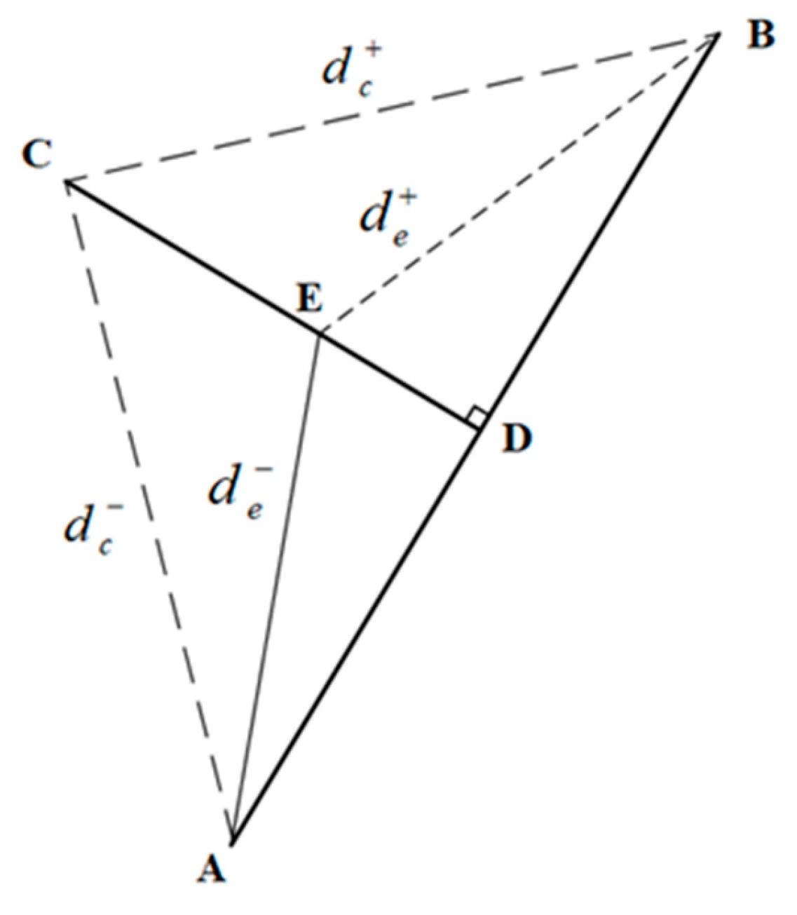
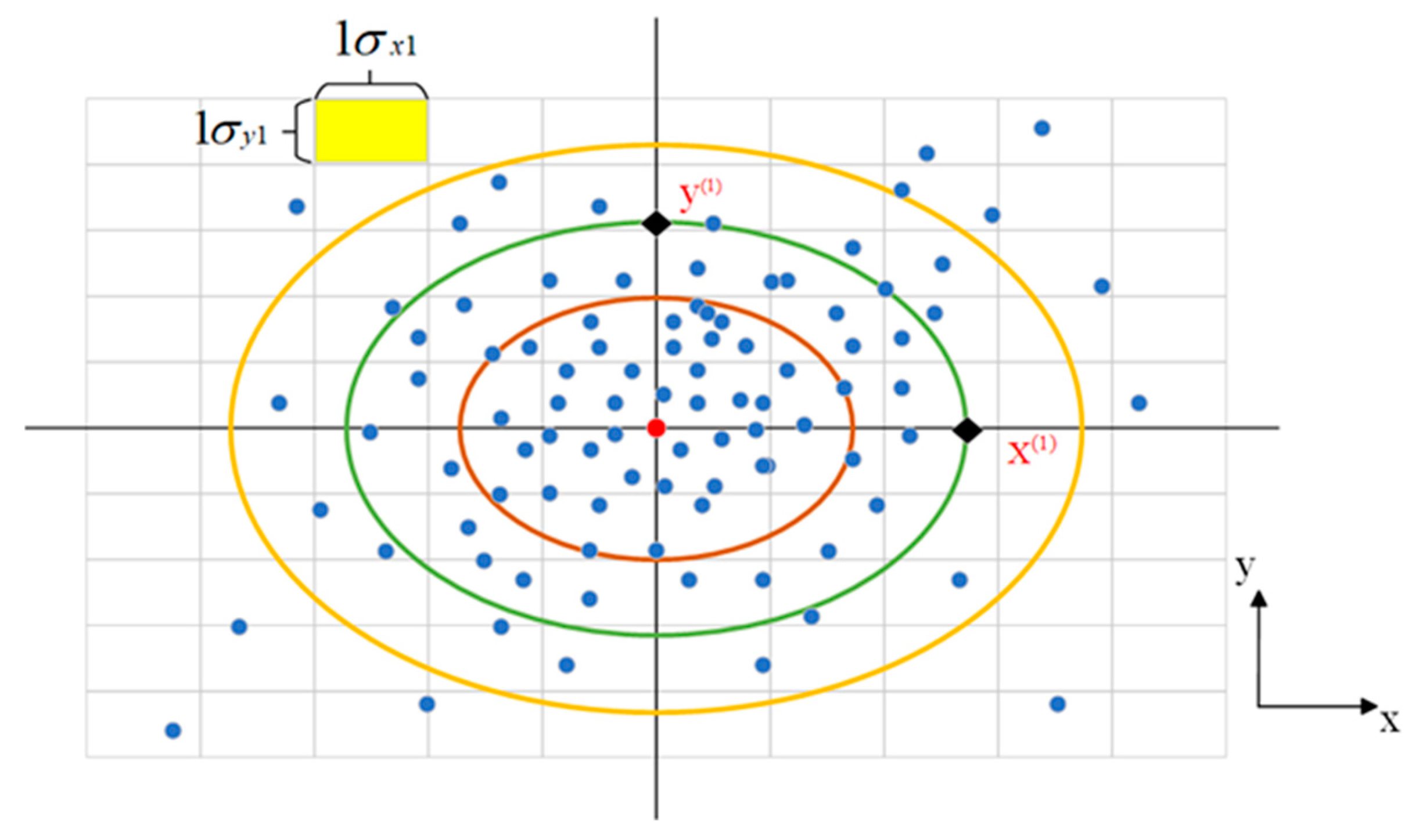
2.3.2. The Modified TOPSIS

The TOPSIS is widely used in comprehensive evaluation systems due to its advantages of flexibility, wide applicability, and strong comprehensiveness. However, it still faces challenges such as unreasonable weight allocation and the inability to handle inconsistency. This is particularly evident in the calculation of distances. When a project scheme is close to both the positive and negative ideal solutions, the TOPSIS method may not provide a very objective evaluation of its merits and demerits. As shown in Figure 4, if points A and B represent the positive and negative ideal solutions, respectively, then any point on the axis CD between AB will have the same distance to points A and B, $d_e^{+}=d_e^{-}$, $d_c^{+}=d_c^{-}$. This would result in all projects having a distance of 0.5 to both the positive and negative ideal solutions, making it impossible to make a fair judgment. Moreover, due to the complexity of evaluating power transmission and transformation projects, the units for evaluation indicators under the economic benefit criteria layer are mostly in thousands of CNY, while those under the carbon reduction benefit criteria layer are mostly in g/kwh. The significant differences in the dimensions of evaluation indicators may lead to considerable discrepancies between the evaluation results and the actual engineering situation when using Euclidean distance calculation.

To address this issue, it is necessary to modify and improve the method, and many scholars have undertaken research in this direction. The authors of [48] comprehensively evaluated the production using traditional TOPSIS, cross entropy, and cosine similarity. The authors of [49] evaluated the testability of radar equipment using the Kullback–Leibler (KL) distance instead of the Euclidean distance. In the aforementioned improvement methods, cosine similarity is not suitable for high-dimensional data. The KL distance method requires the distributions to have the same support domain. The comprehensive evaluation system for carbon reduction benefits in power transmission and transformation projects established in this paper involves numerous evaluation indicators and spans a wide range of evaluation directions, making it unsuitable for the aforementioned improvement methods.

Therefore, adopting standardized Euclidean distance to replace the traditional Euclidean distance in the TOPSIS method. As shown in Figure 5, the normal distributions in the x-direction and y-direction are not the same. Different indicator data are distributed in space as blue dots. The red dot serves as the center point of the coordinate axis. The distribution in the x-direction is more dispersed, while the distribution in the y-direction is more compact. The variances of the two distributions differ significantly. In this case, the modified TOPSIS method will change the length of one unit distance in the Euclidean distance to one unit variance. This effectively avoids calculation discrepancies caused by inconsistent dimensions.

Equations (24) and (25) describe show the process for positive and negative separation calculations in standardized Euclidean distance, respectively.

$$d_i^{+}=\sqrt{{\displaystyle \sum _{j=1}^n\frac{{(f_{ij}-f_j^{+})}^2}{{\sigma }_j^2}}},i=1,2,\cdots ,m$$

(24)

$$d_i^{-}=\sqrt{{\displaystyle \sum _{j=1}^n\frac{{(f_{ij}-f_j^{-})}^2}{{\sigma }_j^2}}},i=1,2,\cdots ,m$$

(25)

2.3.3. TOPSIS-RSR Model

The rank–sum ratio (RSR) refers to a method of statistical analysis that involves obtaining dimensionless statistics by performing rank substitutions on matrices. The evaluation objects are sorted based on their RSR values, and statistical analysis is conducted accordingly [50]. Since the RSR calculation is entirely based on the specific data derived from the TOPSIS and does not involve subjective judgment, it mitigates the subjectivity in decision making to a certain extent. Simultaneously, by computing specific formulas to calculate probabilities, it quantifies the relationship strength between weights. Figure 6 illustrates the specific computational process of the RSR method.

3. Results and Discussion

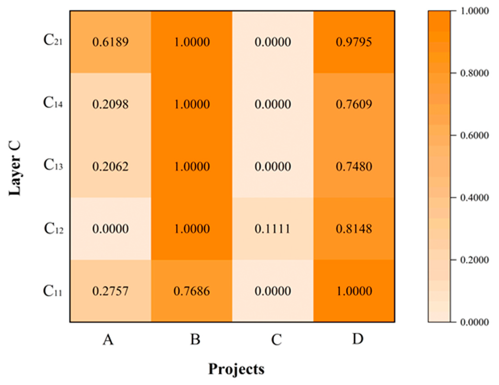
3.1. Cases Study

Data collected from the literature and engineering documents were used to evaluate 220 kV power transmission and transformation projects in four regions: Alashanyouqi (Project A), Dulan (Project B), Jingyu (Project C), and Tangshan (Project D). The specific calculation data can be found in

Table 3. Basic parameters for evaluation on power transmission and transformation projects.

Data	Project A	Project B	Project C	Project D
Internal rate of return/%	12.51	17.39	11.53	11.47
Investment payback period/year	8.9	7.89	11.69	8.7
Return on investment/%	9.4	22.23	18.13	5.8
Asset-liability ratio/%	14.04	25.67	67	39.65
Current ratio/%	1.34	1.57	0.81	1.34
Quick ratio/%	1.21	1.4	0.73	1.01
Electricity sales volume in year (i − 1) /billion·kWh−1	2.6243	4.612	1.269	2.133
Electricity sales volume in year i/billion·kWh−1	2.8104	5.362	2.133	4.59
Overall line loss rate/%	4.69	4.69	4.69	4.69
Grid connection and absorption ratio/%	96	97	96	96
Average coal consumption for power supply/g·kWh−1	326	326	326	326
CO2 emission factor	2.77	2.77	2.77	2.77
SF6 gas emissions/t	480	750	510	700
SF6 gas recovery rate/%	95	95	95	95
SF6 gas conversion factor	23,700	23,700	23,700	23,700
CO2 gas recovery rate/%	80	80	80	80
Installed capacity of thermal power units/%	52	52	52	52
Percentage of carbon emissions reduced by enterprises in the carbon trading market/%	33	33	33	33

.

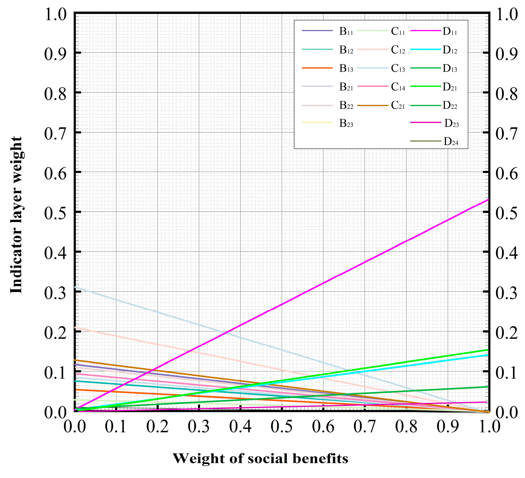
3.2. Combined Weight Analysis

The scoring rules are primarily based on relevant guidelines and manuals, supplemented by relevant literature and the long-term work experience of experts. Obtain the fuzzy judgment matrix using the nine-scale method Q = (q_ij)_m×n.

$$Q=\left[\begin{array}{ccc}{B}_{11}& B_{12}& B_{13}\\ B_{21}& B_{22}& B_{23}\\ B_{31}& B_{32}& B_{33}\end{array}\right]$$

(26)

$$B_{11}=\left[\begin{array}{cccccc}0.5& 0.53& 0.53& 0.382& 0.325& 0.439\\ 0.47& 0.5& 0.53& 0.325& 0.231& 0.382\\ 0.47& 0.47& 0.5& 0.325& 0.231& 0.382\\ 0.618& 0.675& 0.675& 0.5& 0.47& 0.53\\ 0.675& 0.769& 0.769& 0.53& 0.5& 0.53\\ 0.561& 0.618& 0.618& 0.47& 0.47& 0.5\end{array}\right]$$

(27)

$$B_{21}=\left[\begin{array}{cccccc}0.231& 0.325& 0.325& 0.138& 0.138& 0.231\\ 0.325& 0.47& 0.47& 0.231& 0.231& 0.325\\ 0.47& 0.35& 0.35& 0.439& 0.325& 0.47\\ 0.439& 0.47& 0.47& 0.325& 0.231& 0.382\\ 0.439& 0.47& 0.47& 0.325& 0.231& 0.382\end{array}\right]$$

(28)

$$B_{31}=\left[\begin{array}{cccccc}0.439& 0.47& 0.47& 0.231& 0.138& 0.325\\ 0.325& 0.382& 0.382& 0.119& 0.1& 0.138\\ 0.231& 0.325& 0.325& 0.1& 0.1& 0.119\\ 0.382& 0.439& 0.439& 0.138& 0.119& 0.231\\ 0.138& 0.231& 0.231& 0.1& 0.1& 0.1\\ 0.382& 0.439& 0.439& 0.138& 0.119& 0.231\\ 0.382& 0.439& 0.439& 0.138& 0.119& 0.231\end{array}\right]$$

(29)

$$B_{12}=\left[\begin{array}{ccccc}0.769& 0.675& 0.53& 0.561& 0.561\\ 0.675& 0.53& 0.47& 0.53& 0.53\\ 0.675& 0.53& 0.47& 0.53& 0.53\\ 0.862& 0.769& 0.561& 0.675& 0.675\\ 0.862& 0.769& 0.675& 0.769& 0.769\\ 0.769& 0.675& 0.53& 0.618& 0.618\end{array}\right]$$

(30)

$$B_{22}=\left[\begin{array}{ccccc}0.5& 0.382& 0.231& 0.325& 0.325\\ 0.618& 0.5& 0.138& 0.231& 0.5\\ 0.769& 0.862& 0.5& 0.318& 0.675\\ 0.675& 0.769& 0.382& 0.5& 0.561\\ 0.675& 0.5& 0.325& 0.439& 0.5\end{array}\right]$$

(31)

$$B_{32}=\left[\begin{array}{ccccc}0.47& 0.325& 0.138& 0.231& 0.231\\ 0.382& 0.138& 0.1& 0.119& 0.119\\ 0.325& 0.119& 0.1& 0.1& 0.1\\ 0.439& 0.231& 0.119& 0.138& 0.138\\ 0.231& 0.1& 0.1& 0.1& 0.1\\ 0.439& 0.231& 0.119& 0.138& 0.138\\ 0.439& 0.231& 0.119& 0.138& 0.138\end{array}\right]$$

(32)

$$B_{13}=\left[\begin{array}{ccccccc}0.561& 0.675& 0.769& 0.618& 0.862& 0.618& 0.618\\ 0.53& 0.618& 0.675& 0.561& 0.769& 0.561& 0.561\\ 0.53& 0.618& 0.675& 0.561& 0.769& 0.561& 0.561\\ 0.769& 0.881& 0.9& 0.862& 0.9& 0.862& 0.862\\ 0.862& 0.9& 0.9& 0.881& 0.9& 0.881& 0.881\\ 0.675& 0.862& 0.881& 0.769& 0.9& 0.769& 0.769\end{array}\right]$$

(33)

$$B_{23}=\left[\begin{array}{ccccccc}0.53& 0.618& 0.675& 0.561& 0.769& 0.561& 0.561\\ 0.675& 0.862& 0.881& 0.769& 0.9& 0.769& 0.769\\ 0.862& 0.9& 0.9& 0.881& 0.9& 0.881& 0.881\\ 0.769& 0.881& 0.9& 0.862& 0.9& 0.862& 0.862\\ 0.769& 0.881& 0.9& 0.862& 0.9& 0.862& 0.862\end{array}\right]$$

(34)

$$B_{33}=\left[\begin{array}{ccccccc}0.5& 0.675& 0.769& 0.53& 0.862& 0.675& 0.675\\ 0.325& 0.5& 0.675& 0.439& 0.675& 0.53& 0.53\\ 0.231& 0.325& 0.5& 0.382& 0.618& 0.5& 0.5\\ 0.47& 0.561& 0.618& 0.5& 0.862& 0.675& 0.769\\ 0.138& 0.325& 0.382& 0.138& 0.5& 0.231& 0.325\\ 0.325& 0.47& 0.5& 0.325& 0.769& 0.5& 0.439\\ 0.325& 0.47& 0.5& 0.231& 0.675& 0.561& 0.5\end{array}\right]$$

(35)

Based on the FAHP, the subjective weight of criterion can be obtained as w_F. And w_F = (0.0609, 0.0572, 0.0570, 0.0696, 0.0723, 0.0663, 0.0502, 0.0579, 0.0661, 0.0634, 0.0618, 0.0527, 0.0452, 0.0418, 0.0496, 0.0368, 0.0457, 0.0455). Consequently, it can be inferred that the weights derived from FAHP identify “Current ratio B₂₂”, “Asset to liability ratio B₂₁”, and “Quick ratio B₂₃” as the top three indicators. These indicators are all categorized under Layer B, suggesting that, according to experts, economic performance significantly influences carbon reduction initiatives in power transmission and distribution engineering projects.

According to the calculation of EWM, the original parameters of various indicators for the four projects are processed for dimensionless normalization. Figure 7 and Figure 8 illustrate the dimensionless matrices for the economic benefit criterion B and the carbon reduction benefit criterion C.

Under the EWM, the objective weights of each criterion can be obtained as w_E. And w_E = (0.1241, 0.0993, 0.1017, 0.0308, 0.0286, 0.1044, 0.1008, 0.1063, 0.1020, 0.1000). Consequently, it can be inferred that the weights calculated through the objective method EWM rank the top three indicators as follows: “Internal Rate of Return B₁₁”, “Adopting distributed energy generation C₁₃”, and “Participation in carbon trading markets C₁₄”.

The combined weights of indicators at each sub-criterion layer are calculated according to Equation (15). Since the indicators under the social benefit criterion layer are all qualitative indicators, to ensure the normalization of the final combined weights, we use the square of the subjective weights for calculation. The combined weights w of each sub-criterion layer have been obtained. And w = (0.0775, 0.0672, 0.0679, 0.0413, 0.0406, 0.0742, 0.0634, 0.0700, 0.0732, 0.0717, 0.0701, 0.0470, 0.0403, 0.0373, 0.0443, 0.0328, 0.0408, 0.0406).

According to Figure 9, in layer B, the indicator “Internal rate of return B₁₁” has the highest weight. This indicates that the indicator “Internal rate of return B₁₁” plays a significant role in the “Economic benefits B”. In layer C, the indicator “Adoption of Distributed Energy Generation C₁₃” has the highest proportion. This indicates that the indicator “Adoption of Distributed Energy Generation C₁₃” plays a significant role in “Carbon reduction benefits C”. In layer D, the distribution of various indicators is relatively even, with the indicator “Impact on resident income D₁₁” accounting for a significant proportion. This indicates that the indicator “Impact on resident income D₁₁” plays a significant role in “Social benefits D”. In the future, if enterprises aim to improve the comprehensive carbon reduction benefits of power transmission and transformation projects, they should prioritize initiatives based on the above three indicators.

Using the probabilistic module in PySensMCDA [53], a Monte Carlo weights simulation with 1000 runs was conducted to generate criteria weights reflecting the probabilistic approach of criteria relevance distribution. The visualization results are shown in Figure 10.

Figure 11, Figure 12 and Figure 13 illustrate the sensitivity analysis results of economic benefit B, carbon reduction benefit C, and social benefit D. Figure 11 illustrates as the weight of the “Economic benefit” indicator increases, the weights of “Internal rate of return B₁₁”, “Investment payback period B₁₂”, “Return on investment B₁₃”, “Asset to liability ratio B₂₁”, “Current ratio B₂₂”, and “Quick ratio B₂₃” also increase, while the weights of other indicators decrease. This indicates that in the process of carbon reduction construction in power transmission and transformation projects, the more emphasis placed on economic factors, the more likely it is to reap the benefits generated by the six rising indicators. Additionally, the intersection of the two lines in the graph represents the point at which the importance of the two indicators changes. Taking “Internal rate of return B₁₁” and “Using energy-saving wires C₁₁” as an example, before the intersection point, the importance of “Using energy-saving wires C₁₁” is greater than that of “Internal rate of return B₁₁”; meanwhile, after the intersection point, the importance of “Internal rate of return B₁₁” surpasses that of “Using energy-saving wires C₁₁”.

Figure 12 illustrates as the weight of the “Carbon reduction benefit” indicator increases, the weights of “Using energy-saving wires C₁₁”, “Reduce SF₆ gas emissions C₁₂”, “Adopting distributed energy generation C₁₃”, “Participation in carbon trading markets C₁₄”, and “Encourage low-carbon consumption by users C₂₁” also increase, while the weights of other indicators decrease. This indicates that in the process of carbon reduction construction in power transmission and transformation projects, the more emphasis placed on reducing carbon emissions, the more likely it is to reap the benefits generated by the five rising indicators. Additionally, the intersection of the two lines in the graph represents the point at which the importance of the two indicators changes. Taking “Asset to liability ratio B₂₁” and “Encourage low-carbon consumption by users C₂₁” as examples, before the intersection point, the importance of “Asset to liability ratio B₂₁” is greater than that of “Encourage low-carbon consumption by users C₂₁”; meanwhile, after the intersection point, the importance of “Encourage low-carbon consumption by users C₂₁” surpasses that of “Asset to liability ratio B₂₁”. Additionally, with the increase in the weight of the carbon reduction benefit indicator, the weights of “Impact on the natural environment D₂₁” and “Adopting distributed energy generation C₁₃” have the highest slopes, indicating high sensitivity. This suggests that changes in carbon reduction benefits will have a significant impact on these two indicators.

Figure 13 illustrates as the weight of the “Social benefit” indicator increases, the weights of “Impact on residents’ income D₁₁”, “Impact on residents’ quality of life D₁₂”, “Impact on residents’ employment D₁₃”, “Impact on the natural environment D₂₁”, “Impact on local customs and religion D₂₂”, “Impact on local science, education, culture, and health D₂₃”, and “Impact on urbanization development D₂₄” also increase, while the weights of other indicators decrease. This indicates that in the process of carbon reduction construction in power transmission and transformation projects, the more emphasis placed on social impact, the more likely it is to reap the benefits generated by the seven rising indicators. Additionally, the intersection of the two lines in the graph represents the point at which the importance of the two indicators changes. Taking “Reduce SF₆ gas emissions C₁₂” and “Impact on the natural environment D₂₁” as an example, before the intersection point, the importance of “Reduce SF₆ gas emissions C₁₂” is greater than that of “Impact on the natural environment D₂₁”; meanwhile, after the intersection point, the importance of “Impact on the natural environment D₂₁” surpasses that of “Reduce SF₆ gas emissions C₁₂”. Additionally, the indicator “Impact on residents’ income D₁₁” has the highest slope, indicating high sensitivity. This suggests that changes in social benefits will have a significant impact on this indicator.

3.3. Determination of Evaluation Ranks

The TOPSIS method before and after the improvement is used to calculate the project indicators separately, obtaining the relative proximity distance Ci between each project and the optimal solution as shown in Figure 14. Figure 14 illustrates according to the traditional TOPSIS method, Project B has the highest relative closeness degree and the best comprehensiveness, followed by Projects C and D, while Project A has relatively poor comprehensiveness. With the improved TOPSIS method, Projects A and B have relatively high closeness degrees and good comprehensiveness, while Projects C and D perform relatively poorly.

According to the RSR method flowchart for calculation, the RSR distribution and corresponding probability unit values were obtained. Finally, the last cumulative frequency was corrected according to (1-1/4n). The traditional RSR calculation results are shown in

Table 4. Traditional RSR distribution and corresponding probability unit values.

Project	RSR	F	∑f	p	Probit
A	0.5000	2	2	0.5000	5.0000
B	0.9998	4	4	0.9375	6.5341
C	0.4089	1	1	0.2500	4.3255
D	0.5699	3	3	0.7500	5.6744

, And the improved RSR calculation results are shown in

Table 5. Improved RSR distribution and corresponding probability unit values.

Project	RSR	f	∑f	p	Probit
A	0.9999	4	4	0.9375	6.5341
B	0.9991	3	3	0.7500	5.6744
C	0.6263	2	2	0.5000	5.0000
D	0.4571	1	1	0.2500	4.3255

.

Using MATLAB R2023a for fitting calculation with Probit values as independent variables and RSR values as dependent variables, the following linear regression equation is obtained:

$$\mathrm{Traditional} \mathrm{TOPSIS}: y^{*}=-0.773+0.253Probit$$

(36)

$$\mathrm{Improved} \mathrm{TOPSIS}: y=-0.673+0.268Probit$$

(37)

In traditional TOPSIS, the test statistic of the regression equation shows F = 12.201, while its test value p = 0.067, which is greater than 0.05. This indicates that the model is ineffective. In contrast, the improved TOPSIS exhibited a significant regression relationship, with a test statistic of F = 12.201 and a test value of p = 0.043, indicating significance at the 0.05 level. Furthermore, the improved model has an R² value of 0.859, close to 1, indicating a good fit of the curve regression. The VIF value is 1, which is less than the standard value of 5, indicating that there is no multicollinearity issue in the model, and the model construction is well.

The estimated RSR values calculated using Equation (37) is used to classify the evaluation objects into different ranks, dividing the 220 kV power transmission and transformation projects into four levels. The specific classification and C_i are shown in

Table 6. Ranking of power transmission and transformation projects by grades.

Level	The RSR Fitted Values	The RSR Classification Range	The Classification Results
1	1.0791	<0.2655	—
2	0.8486	0.2655~	C, D
3	0.6677	0.6678~	B
4	0.4869	1.07~	A

as follows.

The C_i obtained from TOPSIS and the fitted RSR values obtained from the rank–sum ratio are subjected to fuzzy processing. The fuzzy joint calculation results of each project obtained from the TOPSIS-RSR method are shown in

Table 7. TOPSIS-RSR fuzzy evaluation results.

Projects	Ci	The RSR Fitted Values	TOPSIS-RSR Joint Values	Ranking	Level
A	0.4749	1.0791	0.7770	1	4
B	0.4736	0.8486	0.6611	2	3
C	0.2697	0.6677	0.4687	3	2
D	0.0350	0.4869	0.2609	4	2

.

Overall, considering Table 6 and Table 7, the evaluation results obtained from TOPSIS, RSR, and the combined TOPSIS-RSR for the four projects remain consistent. In the comprehensive efficiency evaluation system of power transmission and transformation projects in four regions, Project A performs the best, followed by Projects B and C, with Project D performing the least favorably. The proposed improved TOPSIS-RSR method effectively avoids the errors in evaluation results caused by the non-uniform dimensions of economic benefits and carbon reduction benefits, which are common in traditional TOPSIS methods. This made the evaluation results more objective, aligning better with the actual engineering situations. The application of the improved TOPSIS-RSR method to rank and grade the comprehensive carbon reduction benefits of the power transmission and transformation projects can provide valuable reference for the comprehensive benefit evaluation of power transmission and transformation projects in other regions in the future.

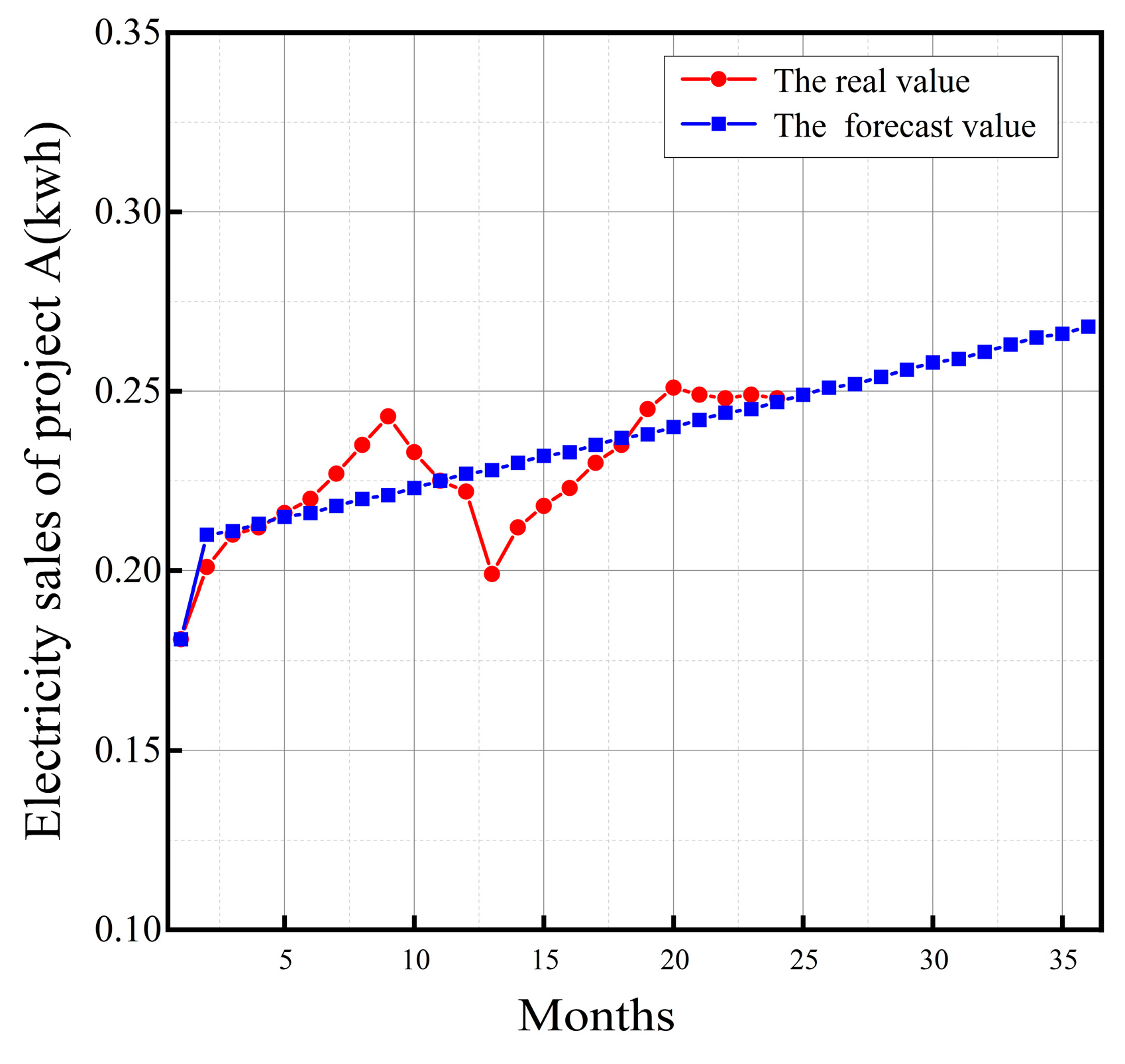
3.4. Forecast of Electricity Sales

To further deepen the analysis of the best-performing Project A, this study uses the electricity sales data from the previous year and the current year as the basis, and conducts a forecast analysis of the electricity sales for the next year on a monthly basis for Project A. Combining the GM (1,1) model, the forecast results are shown in Figure 15. The GM (1,1) grey model [51] was constructed with specific steps, resulting in a development coefficient a of −0.001 and a grey effect quantity b of 1.207. The post-examination residual ratio C value of 0.351 is less than 0.5, indicating the model’s construction accuracy is generally acceptable. Moreover, the average relative error of the model is 3.504%, indicating a good fit of the model. Analysis of Figure 15 reveals that the deviations between the predicted and actual curves mainly occur during the months of July–September each year, possibly due to seasonal peaks in electricity consumption.

4. Conclusions

A comprehensive evaluation system for the carbon reduction benefits of power transmission and transformation projects has been established, delivering economic benefits, carbon reduction benefits, and social benefits. We verified the evaluation model using actual project data from four regions, resulting in the following conclusions:

(a)

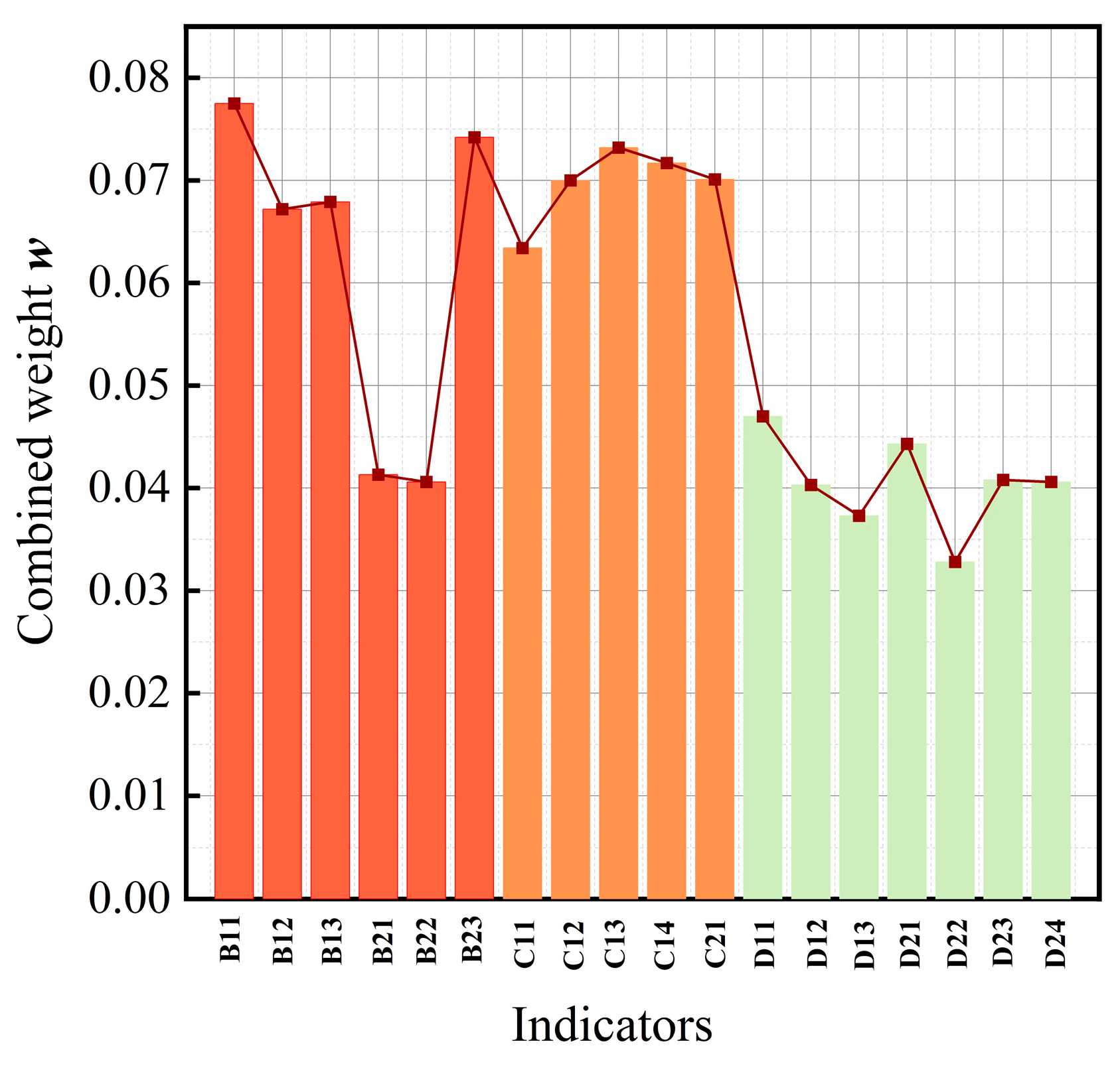
A comprehensive evaluation system for carbon reduction benefits in power transmission and transformation engineering, encompassing economic, carbon reduction, and social benefits has been established. The evaluation system revealed that the most significant indicator in economic benefit B is “Internal Rate of Return B₁₁”, accounting for 7.75% of the combined weight. In carbon reduction benefit C, the most significant indicator is “Adoption of Distributed Energy C₁₃”, constituting 7.32% of the combined weight. Lastly, in social benefit D, the most significant indicator is “Impact on Residents’ IncomeD₁₁”, representing 4.7% of the combined weight.

(b)

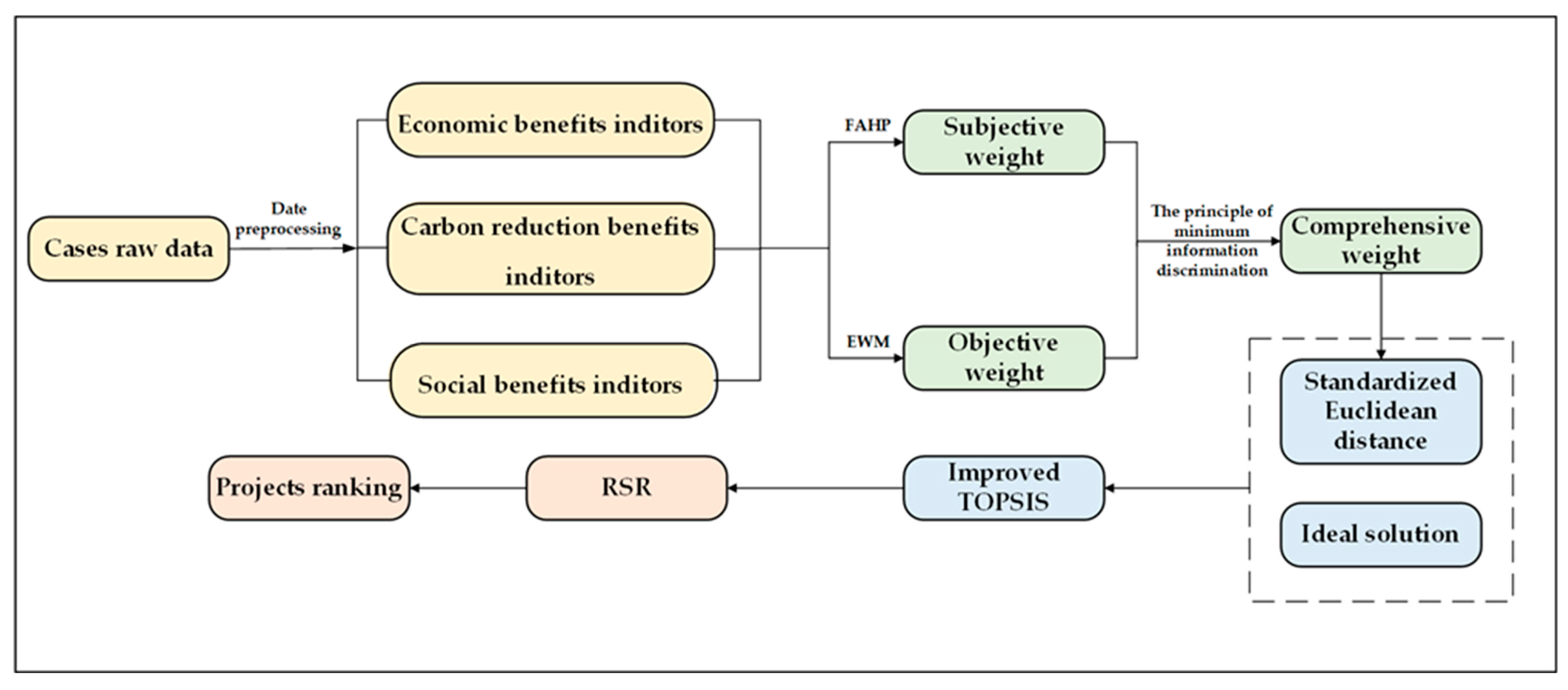
Introducing the TOPSIS-RSR to correct the subjectivity in the combined weights obtained from the FAHP and EWM can make the evaluation results more objective and comprehensive. Finally, using the GM (1,1) model to forecast the electricity sales of the optimal project A, a post-examination residual ratio C of 0.351 was obtained, indicating a good fit of the model.

(c)

While retaining the application of the TOPSIS method for deep information retrieval, the introduction of the RSR method for ranking, along with the modification of the Euclidean distance in traditional TOPSIS to standard Euclidean distance, alleviates the impact of dimensional disparities between economic and carbon reduction benefits on the evaluation results. The traditional TOPSIS method yielded a test value of p = 0.067, whereas the improved TOPSIS method resulted in a test value of p = 0.043 and an R-squared value of 0.859. Thus, the superiority of the improved TOPSIS method in linear regression of the model’s data has been validated.

References

1. Ma, Z.; Zhang, H.; Zhao, H.; Wang, M.; Sun, Y.; Sun, K. New Mission and Challenge of Power Distribution and Consumption System Under Dual-carbon Target. Zhongguo Dianji Gongcheng Xuebao Proc. Chin. Soc. Electr. Eng. 2022, 42, 6931–6944. [Google Scholar]
2. Li, Y.; Xia, Z.; Yang, Q.; Wang, L.; Xing, Y. Review on g-C3N4-based S-scheme heterojunction photocatalysts. J. Mater. Sci. Technol. 2022, 125, 128–144. [Google Scholar] [CrossRef]
3. Acaroğlu, H.; Güllü, M.; Sivri, N.; Garcia Marquez, F.P. How can there be an economic transition to a green ecosystem by adapting plastic-to-fuel technologies through renewable energy? Sustain. Energy Technol. Assess. 2024, 64, 103691. [Google Scholar] [CrossRef]
4. Zhou, Q.; Zhang, J.; Ji, Q.; Liu, Y. Optimization of PCM layer height of cascaded two-layered packed-bed thermal energy storage tank with capsules of varying diameters based on genetic algorithm. J. Energy Storage 2024, 81, 110504. [Google Scholar] [CrossRef]
5. Erasmus, D.J.; Sánchez-González, A.; Lubkoll, M.; Craig, K.J.; von Backström, T.W. Thermal performance characteristics of a tessellated-impinging central receiver. Appl. Therm. Eng. 2023, 229, 120529. [Google Scholar] [CrossRef]
6. Olatoyan, O.J.; Kareem, M.A.; Adebanjo, A.U.; Olawale, S.O.A.; Alao, K.T. Potential use of biomass ash as a sustainable alternative for fly ash in concrete production: A review. Hybrid Adv. 2023, 4, 100076. [Google Scholar] [CrossRef]
7. Osei, A.K.; Rezanezhad, F.; Oelbermann, M. Impact of freeze-thaw cycles on greenhouse gas emissions in marginally productive agricultural land under different perennial bioenergy crops. J. Environ. Manag. 2024, 357, 120739. [Google Scholar] [CrossRef]
8. Dewan, S.; Bamola, S.; Lakhani, A. Addressing ozone pollution to promote United Nations sustainable development goal 2: Ensuring global food security. Chemosphere 2024, 347, 140693. [Google Scholar] [CrossRef]
9. Zhang, C.; Wang, Y.; Xu, J.; Shi, C. What factors drive the temporal-spatial differences of electricity consumption in the Yangtze River Delta region of China. Environ. Impact Asses. 2023, 103, 107247. [Google Scholar] [CrossRef]
10. Gür, T.M. Carbon Dioxide Emissions, Capture, Storage and Utilization: Review of Materials, Processes and Technologies. Prog. Energ. Combust. 2022, 89, 100965. [Google Scholar] [CrossRef]
11. Lei, X.; Zhao, X. The synergistic effect between Renewable Portfolio Standards and carbon emission trading system: A perspective of China. Renew. Energy 2023, 211, 1010–1023. [Google Scholar] [CrossRef]
12. Hansen, T.A.; Wilson, E.J.; Fitts, J.P.; Jansen, M.; Beiter, P.; Steffen, B.; Xu, B.; Guillet, J.; Münster, M.; Kitzing, L. Five grand challenges of offshore wind financing in the United States. Energy Res. Soc. Sci. 2024, 107, 103329. [Google Scholar] [CrossRef]
13. Chen, Y.; Lei, H.; Gao, Z.; Liu, J.; Zhang, F.; Wen, Z.; Sun, X. Energy autonomous electronic skin with direct temperature-pressure perception. Nano Energy 2022, 98, 107273. [Google Scholar] [CrossRef]
14. He, W.; Xu, D.; Zhu, H. Study on the preparation and performance of PVDF/SMA/CdS Fenton-like membrane with both separation and dye degradation functions. J. Ind. Eng. Chem. 2024, in press. [Google Scholar] [CrossRef]
15. Gao, C. Performance investigation of solar-assisted supercritical compressed carbon dioxide energy storage systems. J. Energy Storage 2024, 79, 110179. [Google Scholar] [CrossRef]
16. Chen, N.; Xu, Z.S.; Xia, M.M. The ELECTRE I Multi-Criteria Decision-Making Method Based on Hesitant Fuzzy Sets. Int. J. Inf. Technol. Decis. Mak. 2015, 14, 621–657. [Google Scholar] [CrossRef]
17. Zare Banadkouki, M.R. Selection of strategies to improve energy efficiency in industry: A hybrid approach using entropy weight method and fuzzy TOPSIS. Energy 2023, 279, 128070. [Google Scholar] [CrossRef]
18. Liu, S.; Dong, F.; Hao, J.; Qiao, L.; Guo, J.; Wang, S.; Luo, R.; Lv, Y.; Cui, J. Combination of hyperspectral imaging and entropy weight method for the comprehensive assessment of antioxidant enzyme activity in Tan mutton. Spectrochim. Acta Part A Mol. Biomol. Spectrosc. 2023, 291, 122342. [Google Scholar] [CrossRef]
19. Chen, M.J.M. Research on entropy weight multiple criteria decision-making evaluation of metro network vulnerability. Int. Trans. Oper. Res. 2024, 31, 979–1003. [Google Scholar] [CrossRef]
20. Wang, Y.; Liu, P.; Yao, Y. BMW-TOPSIS: A generalized TOPSIS model based on three-way decision. Inf. Sci. 2022, 607, 799–818. [Google Scholar] [CrossRef]
21. Gebrehiwet, T.; Luo, H. Risk Level Evaluation on Construction Project Lifecycle Using Fuzzy Comprehensive Evaluation and TOPSIS. Symmetry 2019, 11, 12. [Google Scholar] [CrossRef]
22. Cao, J.; Xu, F. Entropy-based fuzzy TOPSIS method for investment decision optimization of large-scale projects. Comput. Intell. Neurosci. 2022, 2022, 4381293. [Google Scholar] [CrossRef]
23. Nandi, R.; Mondal, S.; Mandal, J.; Bhattacharyya, P. From fuzzy-TOPSIS to machine learning: A holistic approach to understanding groundwater fluoride contamination. Sci. Total Environ. 2024, 912, 169323. [Google Scholar] [CrossRef]
24. Fahmi, A.; Khan, A.; Abdeljawad, T.; Alqudah, M.A. Natural gas based on combined fuzzy TOPSIS technique and entropy. Heliyon 2024, 10, e23391. [Google Scholar] [CrossRef]
25. Ali, S.I.; Lalji, S.M.; Hashmi, S.; Awan, Z.; Iqbal, A.; Al-Ammar, E.A.; Gull, A. Risk quantification and ranking of oil fields and wells facing asphaltene deposition problem using fuzzy TOPSIS coupled with AHP. Ain Shams Eng. J. 2024, 15, 102289. [Google Scholar] [CrossRef]
26. Watrobski, J.; Baczkiewicz, A.; Ziemba, E.; Salabun, W. Sustainable cities and communities assessment using the DARIA-TOPSIS method. Sustain. Cities Soc. 2022, 83, 103926. [Google Scholar] [CrossRef]
27. Stoilova, S. Application of simus method for assessment alternative transport policies for container carriage. In Proceedings of the 18th International Scientific Conference on Engineering for Rural Development (ERD), Jelgava, Latvia, 22–24 May 2019; Malinovska, L., Osadcuks, V., Eds.; pp. 898–906. [Google Scholar]
28. Shekhovtsov, A.; Kizielewicz, B.; Sałabun, W. Advancing individual decision-making: An extension of the characteristic objects method using expected solution point. Inf. Sci. 2023, 647, 119456. [Google Scholar] [CrossRef]
29. Dezert, J.; Tchamova, A.; Han, D.; Tacnet, J. IEEE The SPOTIS Rank Reversal Free Method for Multi-Criteria Decision-Making Support. In Proceedings of the 2020 23rd International Conference on Information Fusion (Fusion 2020), Rustenburg, South Africa, 6–9 July 2020; pp. 195–202. [Google Scholar]
30. Xie, X.; Zhang, J.; Lian, Y.; Lin, K.; Gao, X.; Lan, T.; Luo, J.; Song, F. Cloud model combined with multiple weighting methods to evaluate hydrological alteration and its contributing factors. J. Hydrol. 2022, 610, 127794. [Google Scholar] [CrossRef]
31. Song, F.; Tong, S. Comprehensive evaluation of the transformer oil-paper insulation state based on RF-combination weighting and an improved TOPSIS method. Glob. Energy Interconnect. 2022, 5, 654–665. [Google Scholar] [CrossRef]
32. Liu, B.; Yu, X.; Chen, J.; Wang, Q. Air pollution concentration forecasting based on wavelet transform and combined weighting forecasting model. Atmos. Pollut. Res. 2021, 12, 101144. [Google Scholar] [CrossRef]
33. Liu, Z.; Huang, B.; Hu, X.; Du, P.; Sun, Q. Blockchain-Based Renewable Energy Trading Using Information Entropy Theory. IEEE Trans. Netw. Sci. Eng. 2023, 1–12. [Google Scholar] [CrossRef]
34. Liu, Z.; Huang, B.; Li, Y.; Sun, Q.; Pedersen, T.B.; Gao, D.W. Pricing Game and Blockchain for Electricity Data Trading in Low-Carbon Smart Energy Systems. IEEE Trans. Ind. Inform. 2024, 20, 6446–6456. [Google Scholar] [CrossRef]
35. Yang, H.; Chen, Y. Lyapunov stability of fuzzy dynamical systems based on fuzzy-number-valued function granular differentiability. Commun. Nonlinear Sci. 2024, 133, 107984. [Google Scholar] [CrossRef]
36. Santiago, L.; Bedregal, B. Multidimensional fuzzy sets: Negations and an algorithm for multi-attribute group decision making. Int. J. Approx. Reason. 2024, 169, 109171. [Google Scholar] [CrossRef]
37. de Andrade, A.E.R.; Wasques, V.F. The Interactive Fuzzy Semigroup (RIC,+1/2) and its Algebraic Structure Properties. Fuzzy Set. Syst. 2024, 468, 108970. [Google Scholar] [CrossRef]
38. Savari, M.; Shokati Amghani, M. SWOT-FAHP-TOWS analysis for adaptation strategies development among small-scale farmers in drought conditions. Int. J. Disaster Risk Reduct. 2022, 67, 102695. [Google Scholar] [CrossRef]
39. Ahmad, R.; Gabriel, H.F.; Alam, F.; Zarin, R.; Raziq, A.; Nouman, M.; Young, H.V.; Liou, Y. Remote sensing and GIS based multi-criteria analysis approach with application of AHP and FAHP for structures suitability of rainwater harvesting structures in Lai Nullah, Rawalpindi, Pakistan. Urban Clim. 2024, 53, 101817. [Google Scholar] [CrossRef]
40. Thapar, S.S.; Sarangal, H. Quantifying reusability of software components using hybrid fuzzy analytical hierarchy process (FAHP)-Metrics approach. Appl. Soft Comput. 2020, 88, 105997. [Google Scholar] [CrossRef]
41. Więckowski, J.; Kizielewicz, B.; Shekhovtsov, A.; Sałabun, W. RANCOM: A novel approach to identifying criteria relevance based on inaccuracy expert judgments. Eng. Appl. Artif. Intell. 2023, 122, 106114. [Google Scholar] [CrossRef]
42. Yu, X.; Qian, L.; Wang, W.E.; Hu, X.; Dong, J.; Pi, Y.; Fan, K. Comprehensive evaluation of terrestrial evapotranspiration from different models under extreme condition over conterminous United States. Agric. Water Manag. 2023, 289, 108555. [Google Scholar] [CrossRef]
43. Han, H.; Li, X.; Gu, X.; Li, G. Urban rivers health assessment based on the concept of resilience using improved FCM-EWM-MABAC model. Ecol. Indic. 2023, 154, 110833. [Google Scholar] [CrossRef]
44. Li, Y.; Lu, C.; Liu, G.; Chen, Y.; Zhang, Y.; Wu, C.; Liu, B.; Shu, L. Risk assessment of wetland degradation in the Xiong’an New Area based on AHP-EWM-ICT method. Ecol. Indic. 2023, 153, 110443. [Google Scholar] [CrossRef]
45. Luo, Z.; Tian, J.; Zeng, J.; Pilla, F. Flood risk evaluation of the coastal city by the EWM-TOPSIS and machine learning hybrid method. Int. J. Disaster Risk Reduct. 2024, 106, 104435. [Google Scholar] [CrossRef]
46. Wang, J.; Gu, C.; Liu, K. Anomaly electricity detection method based on entropy weight method and isolated forest algorithm. Front. Energy Res. 2022, 10, 984473. [Google Scholar]
47. Wang, S.; Ge, L.; Cai, S.; Wu, L. Hybrid interval AHP-entropy method for electricity user evaluation in smart electricity utilization. J. Mod. Power Syst. Clean Energy 2018, 6, 701–711. [Google Scholar] [CrossRef]
48. Zhang, J.; Xu, L.; Xia, L.; Yang, Q.; Chen, Z.; Dong, W. Comprehensive Evaluation Technology of Photovoltaic Power Station Power Generation Performance Based on Minimum Deviation Combined Weighting Method. In Proceedings of the 2022 IEEE 6th Conference on Energy Internet and Energy System Integration (EI2), Chengdu, China, 11–13 November 2022; pp. 880–885. [Google Scholar]
49. Ongena, S.; Paraschiv, F.; Reite, E.J. Counteroffers and Price Discrimination in Mortgage Lending. J. Empir. Financ. 2023, 74, 101431. [Google Scholar] [CrossRef]
50. Kelemenis, A.; Askounis, D. A new TOPSIS-based multi-criteria approach to personnel selection. Expert. Syst. Appl. 2010, 37, 4999–5008. [Google Scholar] [CrossRef]
51. Ilham, N.I.; Dahlan, N.Y.; Hussin, M.Z. Optimizing solar PV investments: A comprehensive decision-making index using CRITIC and TOPSIS. Renew. Energy Focus 2024, 49, 100551. [Google Scholar] [CrossRef]
52. Wang, Y.; Hong, L.; Liu, Z.; Sun, L.; Liu, L. Rheological performance evaluation of activated carbon powder modified asphalt based on TOPSIS method. Case Stud. Constr. Mater. 2024, 20, e2963. [Google Scholar] [CrossRef]
53. Paradowski, B.; Więckowski, J.; Sałabun, W. PySensMCDA: A novel tool for sensitivity analysis in multi-criteria problems. Softwarex 2024, 27, 101746. [Google Scholar] [CrossRef]
Figure 1. Benefit evaluation flowchart.
Energies 17 02988 g001
Figure 2. FAHP method calculation process.
Energies 17 02988 g002
Figure 3. Calculation process of EMW.
Energies 17 02988 g003
Figure 4. Shortcomings of the traditional TOPSIS method.
Energies 17 02988 g004
Figure 5. The modified TOPSIS.
Energies 17 02988 g005
Figure 6. RSR method calculation process.
Energies 17 02988 g006
Figure 7. The dimensionless matrix for layer B based on EWM.
Energies 17 02988 g007
Figure 8. The dimensionless matrix for layer C based on EWM.
Energies 17 02988 g008
Figure 9. Combined weights of indicators in the evaluation system of comprehensive benefit of carbon reduction in power transmission and transformation projects.
Energies 17 02988 g009
Figure 10. Visualization of values distribution of weights generated with Monte Carlo simulations.
Energies 17 02988 g010
Figure 11. Sensitivity analysis of economic benefits.
Energies 17 02988 g011
Figure 12. Sensitivity analysis of carbon reduction benefits.
Energies 17 02988 g012
Figure 13. Sensitivity analysis of social benefits.
Energies 17 02988 g013
Figure 14. Ci of the TOPSIS method before and after improvement.
Energies 17 02988 g014
Figure 15. GM (1,1) method for electricity sales forecasting.
Energies 17 02988 g015