Thermostratigraphic and Heat Flow Assessment of the South Slave Region in the Northwest Territories, Canada

Abstract

Despite the elevated heat flow known in the Western part of the South Slave Region (Northwest Territories, Canada), a continuous and equilibrium geothermal gradient was never measured in boreholes below the communities where geothermal energy could be developed. This paper aims to predict the geothermal gradient and assess the Earth’s natural heat flow below the communities of Fort Providence, Kakisa, Hay River, and Enterprise. Temperatures from drill-stem tests and bottom well logs were corrected for drilling disturbance and paleoclimate. The thermal conductivity and heat generation rate of the geological formations were determined from the literature and with new laboratory measurements. Original 1D models were developed to evaluate subsurface temperature through the sedimentary formations based on a thermostratigraphic assessment. The results indicate a geothermal gradient that varies from 44.1 ± 10.6 °C km⁻¹ to 59.1 ± 14.9 °C km⁻¹ and heat flow that varies from 105.5 mW m⁻² to 160.2 mW m⁻² below the communities. These estimates were in agreement with the equilibrium geothermal gradients measured in Cameron Hills, south of the four communities, and were used to verify our predictions. The highest geothermal gradient (59.1 ± 14.9 °C km⁻¹) was estimated at Hay River, which, therefore, has the most favorable geological conditions for geothermal development.

1. Introduction

Estimating the geothermal gradient and terrestrial heat flow are important steps in assessing the geothermal potential of a region. The geothermal gradient is typically estimated based on an equilibrium temperature profile (e.g., [1,2]), and the thermal conductivity of the geological materials underlying the region is measured for heat flow assessment. This kind of heat flow assessment is crucial for any geothermal development, but it can be expensive because it usually requires an exploration borehole specifically drilled for geothermal purposes (e.g., [3]). In remote communities of the Canadian North that have populations of a few hundred to less than four thousand people, drilling such boreholes is difficult to justify in the early exploration stage. However, 1D models that rely on a thermostratigraphic assessment and corrected downhole temperatures can be used to predict geothermal gradient and heat flow at this stage (e.g., [1,4,5,6]). This approach can better inform decision-making regarding the exploitability of clean and reliable local geothermal heat for such remote communities.

The geothermal potential of the South Slave Region of the Northwest Territories (NWT) is studied using a community-based approach to evaluate the thermal state and properties below (from North to South) Fort Providence, Kakisa, Hay River, and Enterprise (Figure 1). The most recent map of heat flow in Canada [7,8], modified from Grasby et al. [9], indicates heat flow values in the South Slave Region from 40 mW m⁻² to 100 mW m⁻², which is the highest in the Western Canada Sedimentary Basin (WCSB). The work of EBA Engineering Consultants Ltd. [10] has shown very high geothermal favorability and potential in the NWT to the west of Great Slave Lake (Figure 1b). To support geothermal research in the South Slave Region, Petrel Robertson Consulting Ltd. [11] identified 109 oil and gas wells between 48 m and 1500 m in depth that were cored and have publicly available geoscience data that could be further investigated. Historic well files with bottom-hole temperatures (BHTs) and drill-stem test (DST) records are publicly available for 68 of these wells. Individual well history files from the archives of the Office of the Regulator of Oil and Gas Operations [12] were also consulted to supplement the temperature data. Oil and gas wells were recently abandoned in Cameron Hills, located about 100 km to the southwest of the studied communities. Smejkal et al. [13] accessed these wells during abandonment activities and measured an equilibrium temperature profile in six deep wells and evaluated their geothermal gradient.

Terrestrial heat flow estimates from the analysis of BHT data exist for several sedimentary basins around the world, including Brazil [16], Western Canada [17], Eastern Canada [18], and the St. Lawrence Lowlands in Québec [4]. Drill-stem test temperature based on flowing oil or water from the producing formation is generally a reliable source of data for the calibration of basin system models [19] but is not as common as BHT measurements. On the other hand, BHTs from well log headers are available for most wells but are biased and usually lower than the equilibrium formation temperature [20]. Hence, correction for drilling disturbances is necessary and requires multiple BHT measurements at successive times in order to find the equilibrium temperature. The analytical Horner technique is commonly used to correct multiple BHT measurements [21]. The criteria for reliable Horner-corrected BHTs include a minimum of three logging runs that record time and temperature for each run and deviation from the least squares regression line that is less than the measurement uncertainty (i.e., ± 1–3 °C; [19]). Other corrections that do not use mud circulation time include the Förster Correction [22], the Harrison Correction [6], subsequently redefined by Blackwell et al. [23] and Blackwell [24], and the Kehle Correction [25]. These correction schemes were used for correcting BHTs in the Denver Basin in Colorado and in Nebraska [26]. However, these empirical corrections are not always appropriate as differences in lithologies and thermal histories may affect the correction [26,27]. Heat flow estimates, especially those based on temperature measurements at a shallow depth, additionally require corrections for paleoclimate effects [28]. These effects must be considered in the South Slave Region, which was covered by the Laurentide Ice Sheet during the last glaciation (Late Wisconsinan) ~10–25 ka ago [29,30], resulting in a decrease in subsurface temperature through thermal diffusion.

In this study, our objective is to reevaluate the heat flow and predict the geothermal gradient with original 1D models in the four main South Slave communities that are at an early geothermal exploration stage. This paper provides a widely applicable workflow of local geological assessment that can be used to plan the drilling of exploration boreholes, helping to move to the next step of geothermal development in small and remote communities. Relying on available data, we use a community approach rather than a regional assessment to predict the thermal state and properties below population centers where geothermal energy can be used. We believe it is the most appropriate method for such a remote region where the population is sparse and geothermal energy exportation is hindered by the lack of infrastructure. Our assessment comprises the analysis of publicly available data from oil and gas wells near the four communities and includes BHT and DST data combined with vertical thermal conductivity profiles deduced from core analysis and corresponding lithological profiles beneath the communities. A 1D thermostratigraphic model for each community is developed and verified with equilibrium temperature data obtained from Cameron Hills.

2. Geological Setting

The study area defined within the South Slave Region is delineated by the coordinates 60° N, 111° W in the SE to 62° N, 120° W in the NWT (Figure 1a). This area is located in the Interior Platform, which constitutes the northern extension of the WCSB, and is bounded by the Canadian Shield to the east and the Mackenzie Mountains of Cordilleran Orogen to the west ([30] and references therein). According to Davenport [14], the Interior Platform is divided into a number of domains or exploration areas. This subdivision was based on geological history, physiographic and structural characteristics, and changes in bedrock geology. The area of interest for this study is in the Great Slave Plain (Figure 1a; [31]).

The geology of the Great Slave Plain comprises Precambrian metasedimentary and crystalline basement rocks overlain by Paleozoic and Mesozoic sedimentary rocks and Quaternary overburden with a variable thickness. The dominant lithologies making up the Paleozoic and Mesozoic sedimentary strata are shale, limestone, marine dolostone, anhydrite, and sandstone. Devonian rocks make up the bulk of the sedimentary strata underlying the communities, illustrated by the cross-sections in Figure 2b; for a detailed review and description of the Devonian stratigraphy, see Meijer Drees [32], Moore [33], Morrow et al. [34], and Mossop et al. [35], among others.

According to the work of Gal et al. [36], the local stratigraphy comprises a relatively thin (500 m to 700 m) Paleozoic and Mesozoic sedimentary cover overlying the Precambrian basement (Figure 2b). This is confirmed by the Phanerozoic isopach map of the WCSB [37].

Smith et al. [38] provide the most recent drift isopach model, including the thickness of Quaternary glacial sediment. The drift cover in South Slave is up to 150 m thick but has considerable variation; the majority of the cover is less than 10 m thick, and sedimentary rocks outcrop in the area sporadically. At Cameron Hills, the drift thickness is locally up to 400 m thick.

An extensional tectonic regime in the late Precambrian resulted in deep-seated faults and horst and graben block faulting of basement rocks stretching to the Cameron Hills area. This extensional tectonic regime was reactivated and influenced the Phanerozoic sediment cover. The major faults and fault zones that affected the area have a northeast trend (Figure 2; [36,39]).

Figure 2. (a) Geological map of the study area (modified from [40]). The well locations were taken from the Geothermal Database Compilation Devonian Cores Map from Petrel Robertson Consulting Ltd. [11] and Gal et al. [36]. (b) Cross-sections A-A’ and B-B’ showing stratigraphic and chronological relationships of the dominant lithologies and their corresponding formations in the Great Slave Plain (modified from Gal et al. [36]).

Figure 2. (a) Geological map of the study area (modified from [40]). The well locations were taken from the Geothermal Database Compilation Devonian Cores Map from Petrel Robertson Consulting Ltd. [11] and Gal et al. [36]. (b) Cross-sections A-A’ and B-B’ showing stratigraphic and chronological relationships of the dominant lithologies and their corresponding formations in the Great Slave Plain (modified from Gal et al. [36]).

3. Input Data

The dataset consists of information from 75 of the 116 wells in the area of interest (Figure 3), which were made available from the Petrel Robertson Consulting Ltd. [11] Excel file and the individual well history files from OROGO [12]. Detailed data are available in the Supplementary Material provided with the article. The wells with DST and/or BHT data that were chosen as close as possible to the four main communities. The equilibrium temperature profiles recorded in 2023 from six wells (A-73, E-07, I-10, I-74, L-44, and M-49) in the Cameron Hills region are located close enough to the study area (Figure 3) to be used for verification purposes.

3.1. Temperature Data

3.1.1. South Slave Region

A total of 33 of the 75 wells have a DST temperature record. BHTs were measured in 42 wells at a depth of 504 m to 1657 m (

Table 1. Temperature data from wells.

Data Type	Number of Wells	Depth TVD	Temperature	Source
		[m]	[°C]
DST	20 5	≥600–1846 <600	19–63	Petrel Robertson Consulting Ltd. [11]
	4 3	≥600–941 <600	17–42	OROGO [12]
BHT	36 5	≥600–1657 <600	26–76	Petrel Robertson Consulting Ltd. [11]
	1 1	≥600 <600	27	OROGO [12]
No data	41			Petrel Robertson Consulting Ltd. [11]
Total	116	49–1949	17–76

).

Set as the upper boundary condition in our model, the average annual undisturbed ground temperature T_s (°C) was obtained by converting the air temperature to the ground temperature using an empirical relationship. The following equation developed by Ouzzane et al. [41] was used for this purpose:

T_s = 17.898 + 0.951T_amb,

(1)

where T_s (K) is the undisturbed ground surface temperature and T_amb (K) is the annual ambient temperature, which is −2.5 °C for the region. The mean annual air temperature was obtained from the Hay River-A weather station [42]. T_s was consequently estimated as 2.1 °C.

3.1.2. Cameron Hills

The equilibrium temperature data from wells in Cameron Hills were chosen because the stratigraphy shares similarities with that of the South Slave communities. These similarities were confirmed with the gamma ray (GR) log [13]. The stratigraphic formations and corresponding lithologies were taken from the Table of Formation Tops established by Gal et al. [36] and Rocheleau et al. [15]. In Cameron Hills, T_s was evaluated from the temperatures measured at the top of the Cretaceous basal sandstone (CB SS unit), marking the base of the clastic Cretaceous section underlying the Devonian carbonates, since continuous temperature profiles were available at this geological formation at a depth of approximately 500 m [13].

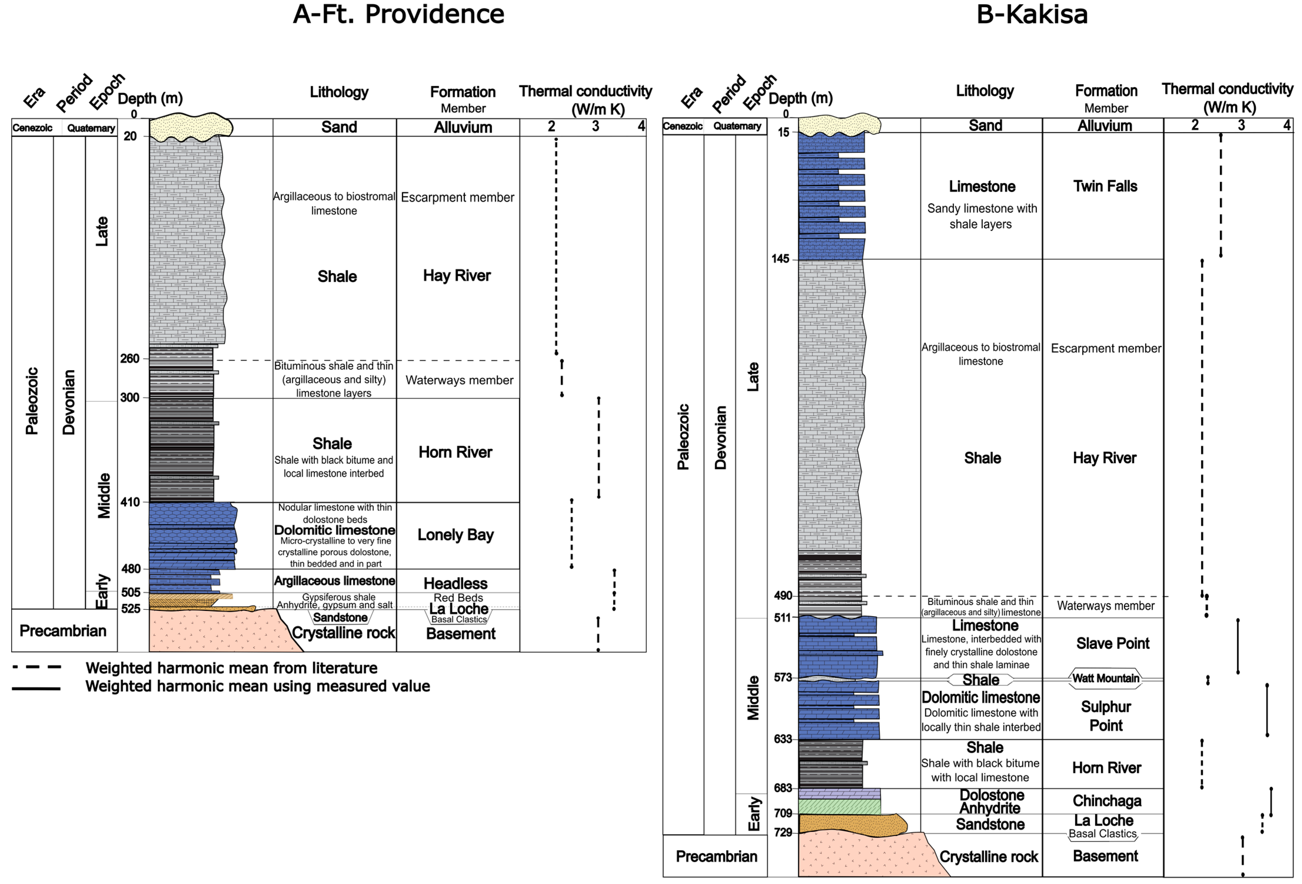
3.2. Thermal Conductivity and Heat Generation Rate

3.2.1. South Slave Region

Thermostratigraphic logs were initially created for the four South Slave communities by combining the stratigraphic column that approximates the thickness of the main stratigraphic formations with the corresponding subsurface thermal conductivity (

Table 2. Thermal conductivity and heat generation rate for South Slave communities.

Formation	Lithology	%	n	Heat Production A [W m−3]	Thermal Conductivity λ [W m−1 K−1]
					Measured	Literature *	Average
Alluvium	Sand	100		0.73 × 10−6		1.4	1.4
Twin Falls	Limestone	95		0.19 × 10−6		2.5	2.5
	Shale	5		0.53 × 10−6		2.1
Hay River	Shale	92		0.53 × 10−6		2.1	2.1
	Limestone	8		0.19 × 10−6		2.5
Hay River (Escarpment)	Shale	90		0.53 × 10−6		2.1	2.1
	Limestone	10		0.19 × 10−6		2.5
Hay River (Waterways)	Shale	60		0.53 × 10−6		2.1	2.2
	Limestone	40		0.19 × 10−6		2.5
Slave Point	Limestone	92	25	0.19 × 10−6	2.9 ± 0.25		2.9
	Shale	4		0.53 × 10−6		2.1
	Dolostone	4	4	0.11 × 10−6	4.6 ± 0.55
Horn River	Shale	95		0.53 × 10−6		2.1	2.1
	Limestone	5		0.19 × 10−6		2.5
Watt Mountain	Shale	92		0.53 × 10−6		2.1	2.2
	Limestone	3	6	0.19 × 10−6	3.1 ± 0.18
	Sandstone	5		0.73 × 10−6		3.4
Sulphur Point	Limestone	78	13	0.19 × 10−6	3.4 ± 0.63		3.5
	Dolostone	20	7	0.11 × 10−6	4.4 ± 0.64
	Shale	2		0.53 × 10−6		2.1
Muskeg	Anhydrite	90	1	0.08 × 10−6	5.0 ± 0.17	3.4	4.4
	Dolostone	10	6	0.11 × 10−6	5.6
Klua	Shale	98		0.53 × 10−6		2.1	2.1
	Limestone	2		0.19 × 10−6		2.5
Keg River	Limestone	90		0.19 × 10−6		2.8	3
	Dolostone	10	8	0.11 × 10−6	4.9 ± 0.47
Lonely Bay	Dolostone	50		0.11 × 10−6		3.8	3
	Limestone	50		0.19 × 10−6		2.5
Chinchaga	Anhydrite	43	2	0.08 × 10−6	4.8 ± 0.77		3.6
	Dolostone	30	4	0.11 × 10−6	4.2 ± 0.80
	Shale	23		0.53 × 10−6		2.1
	Limestone	2		0.19 × 10−6		2.5
Chinchaga (Ebutt Member)	Shale	83		0.53 × 10−6		2.1	3.6
	Limestone	10		0.19 × 10−6		2.5
	Dolostone	5		0.11 × 10−6		3.8
	Anhydrite	2		0.08 × 10−6		4.3
Headless	Limestone	50		0.19 × 10−6		2.5	2.3
	Shale	45		0.53 × 10−6		2.1
	Dolostone	5		0.11 × 10−6		3.8
Mirage Point	Shale	62		0.53 × 10−6		2.1	2.6
	Dolostone	15		0.11 × 10−6		3.8
	Halite	15		0.08 × 10−6		5
	Anhydrite	8		0.08 × 10−6		4.3
Mirage Point (Ernestina Lake)	Dolostone	55		0.11 × 10−6		3.8	3.3
	Anhydrite	25		0.08 × 10−6		4.3
	Shale	20		0.53 × 10−6		2.1
La Loche	Sandstone	99		0.73 × 10−6		3.4	3.4
	Shale	1		0.53 × 10−6		2.1
La Loche (Red Beds)	Sandstone	100		0.73 × 10−6		3.4	3.4
La Loche (Basal Clastics)	Sandstone	100		0.73 × 10−6		3.4	3.4
Precambrian	Granite	100				3

n: number of samples. * Sources (e.g., [9] and references therein, [48,49] and references therein, and [50,51,52,53,54]).

; Figure 4; [43]). The average thermal conductivity per formation was calculated using the weighted harmonic mean related to bedded lithologies, assuming perpendicular heat flow [44]. These local stratigraphic columns gave an extended and refined geological model under each community, showing that the Precambrian basement lies at a shallow depth of 500 m to 700 m. Shale is the dominant lithology over the total thickness of sedimentary rocks (~600 m) in Fort Providence, Kakisa, and Enterprise. The carbonate rocks are 600 m thick, and the shale cover is approximately 100 m thick at the Hay River location. Near the surface, quaternary sediments overlying the Paleozoic rocks are less than 10 m thick and were omitted because the sedimentary deposits do not contribute enough to heat transfer when calculating the geothermal gradient and heat flow from deep rocks (e.g., Beardsmore et al. [45]; Jaupart et al. [46]). A laboratory assessment of the thermal conductivity was completed on 84 split core samples from 33 wells that cover seven geological formations. The measurements were carried out at the Laboratoire ouvert de géothermie at the Institut national de la recherche scientifique (INRS) in Canada using an optical scanning instrument following the methodology of Popov et al. [47]. For some formations, no core was available for measurement; the thermal conductivity was thus obtained from the literature (e.g., [9] and references therein, [48,49] and references therein, and [50,51,52,53,54]) and used in the weighted harmonic mean thermal conductivity calculation of the formation.

The average heat generation rate A (W m⁻³) for lithological formations below the South Slave communities was evaluated using the empirical equation of Bücker et al. [55], which relates heat generation to the concentration of uranium [U], thorium [Th], and potassium [K]. The concentration of these radiogenic elements was determined using inductively coupled plasma analyses at the INRS geochemical laboratory [43]. Although the laboratory measurements were made on the available core material, this was insufficient to cover all the geological formations. Consequently, heat generation rates were assumed to be analogous to lithologically similar formations where they were evaluated. Additionally, the literature values of the heat generation rate (e.g., [56,57] and references therein) were assigned to the sedimentary rock type for formations with no core.

3.2.2. Cameron Hills

Core materials were not available for the wells in Cameron Hills and geological formations encountered there. Thermal conductivity was determined to be similar to thermal conductivity measurements made on core samples for the South Slave formations from Rajaobelison et al. [43] (Table 2; Figure 4).

The internal heat generation rate for rocks A (W m⁻³) intersected by wells in Cameron Hills was calculated from the gamma ray log (GR; American Petroleum Institute units) according to Equation [2] from Burrus et al. [58]:

A = 0.0145 × (GR − 5)

(2)

The average heat production rate for each formation was calculated from the arithmetic average GR measured between the top and the base of each corresponding formation (

Table 3. Thermal conductivity and heat generation rate of geological formations in Cameron Hills.

Well’s Short Name	Geological Formations	Top	Lithology	λ	GR	A
		[m]		[W m−1 K−1]	[API]	[W m−3]
A-73	Wabamun	443	Dolomitic limestone	3.5	49.0	0.64 × 10−6
	Twin Falls	809	Limestone	2.5	34.6	0.43 × 10−6
	Muskwa	1022	Organic-rich shale	2.1	23.5	0.27 × 10−6
	Waterways	1283	Bituminous shale	2.1	11.2	0.09 × 10−6
E-07	CB SS	461.4	Sandstone	3.4	30.7	0.37 × 10−6
	Wabamun	471.9	Dolomitic limestone	3.5	32.5	0.40 × 10−6
	Twin Falls	760	Limestone	2.5	31.8	0.39 × 10−6
	Hay River	912.5	Shale	2.2	60.6	0.81 × 10−6
I-10	CBS SS	575.1	Sandstone	3.4	43.3	0.56 × 10−6
	Wabanum	590.3	Dolomitic limestone	3.5	17.9	0.19 × 10−6
	Trout River	622	Shale	2.1	15.1	0.15 × 10−6
	Kakisa	627.9	Limestone	3.0	16.7	0.17 × 10−6
	Redknife	665.8	Shale	2.1	57.8	0.77 × 10−6
	Tathlina	715	Shale	2.1	35.1	0.44 × 10−6
	Twin Falls	868.3	Limestone	2.5	27.6	0.33 × 10−6
	Hay River	999.5	Shale	2.1	50.5	0.66 × 10−6
I-74	BS SS	539.7	Sandstone	3.4	31.5	0.38 × 10−6
	Wabamun	554.6	Dolomitic limestone	3.5	17.0	0.17 × 10−6
	Ft. Simpson	717.6	Limestone	3.0	39.2	0.50 × 10−6
	Twin Falls	829.1	Limestone	2.5	20.4	0.22 × 10−6
	Hay River	898.8	Shale	2.1	44.5	0.57 × 10−6
L-44	CB SS	516.8	Sandstone	3.4	30.6	0.37 × 10−6
	Wabamun	528.2	Dolomitic limestone	3.5	40.6	0.52 × 10−6
	Twin Falls	855	Limestone	2.2	70.8	0.95 × 10−6
	Hay River	1022	Shale	2.1	68.3	0.92 × 10−6
	Beaverhill Lake	1305.2	anhydrite and Limestone	4.3	49.0	0.64 × 10−6
M-49	CBS SS	471.6	Sandstone	3.4	33.1	0.41 × 10−6
	Wabanum	478.1	Dolomitic limestone	3.5	33.1	0.41 × 10−6
	Ft. Simpson	696.5	Shale	3.0	20.2	0.22 × 10−6
	Twin Falls	812.8	Limestone	2.5	46.5	0.60 × 10−6
	Hay River	961.9	Shale	2.1	32.2	0.39 × 10−6
	Beaverhill Lake	1252.6	Anhydrite and Carbonates	4.3	60.5	0.80 × 10−6
	Slave Point	1301.9	Limestone	2.9	56.6	0.75 × 10−6

).

4. Methods

Input temperature data were corrected for drilling disturbance and paleoclimates. Then, the geothermal gradient was calculated at the location of each community and for the wells in Cameron Hills. The equilibrium temperature profile measured at Cameron Hills was reproduced to verify if the thermal conductivity for each geological formation was adequately assigned. After the verification, the surface heat flow was calculated for the four communities and the 1D temperature profile below the four South Slave communities was predicted without paleoclimate correction using analytical calculations and assuming one-dimensional conductive heat transfer with an internal heat generation in a steady state.

4.1. Drilling Disturbance Correction for BHTs

Of the 75 wells, only 42 had one to two BHTs from wireline logs, and mud circulation time was not provided. This was insufficient to meet the criteria for Horner correction [19]. Empirical corrections were therefore applied to the BHTs following the work of Crowell et al. [26]. The Harrison equation [6], the Kehle equation [59], the Förster (a) equation [22], and the Förster (b) equation [60] were considered for corrections because the lithology of the South Slave Region is similar to that of the basins in which these corrections were developed [e.g., [22,26]]:

T_cf (°C) = − 16.51 + 0.018 × TVD − 2.345 × 10⁻⁶ × TVD²,

(3)

T_cf (°F) = − 8.819 × 10⁻¹² × TVD − 2.143×10⁻⁸ × TVD² + 4.375 × 10⁻³ × TVD − 1.018,

(4)

T_cf (°C) = 0.012 × TVD − 3.68,

(5)

T_cf (°C) = 0.017 × TVD − 6.58.

(6)

where T_cf (°C/°F) is the temperature coefficient correction added to the BHT, and TVD (m/in feet for Kehle equation) is the true vertical depth at which the BHT was measured.

Then, the best correction method was chosen based on the best fit to the geothermal gradient calculated from DST temperatures [22]. The corrections were established for depths of 600 m to 3 km; thus, temperatures recorded in South Slave wells at depths shallower than 600 m were not corrected. However, uncorrected temperatures at depths between 300 m and 600 m were retained when the gradient was evaluated at the community scale to improve the accuracy of the evaluation where data were limited.

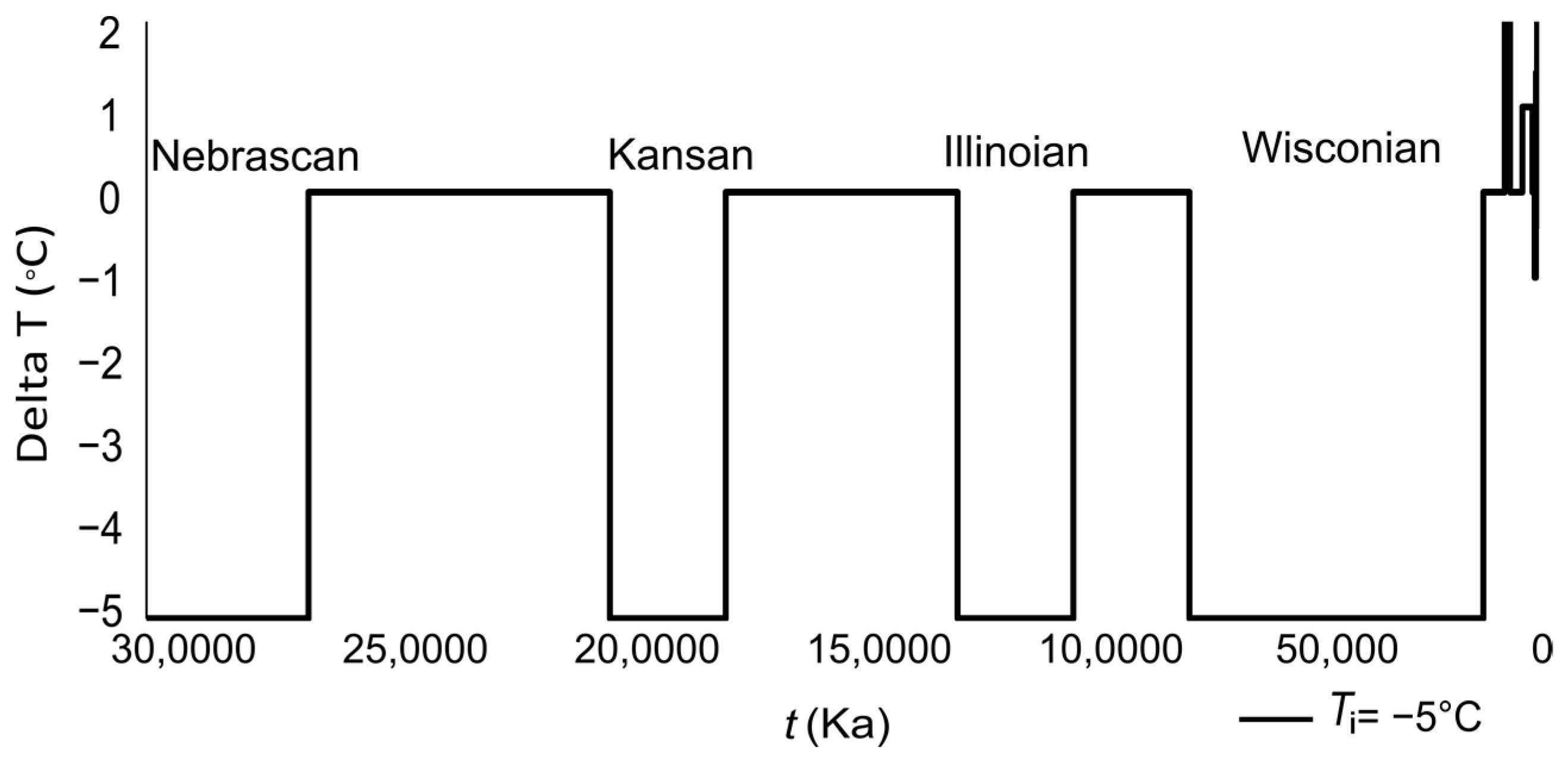
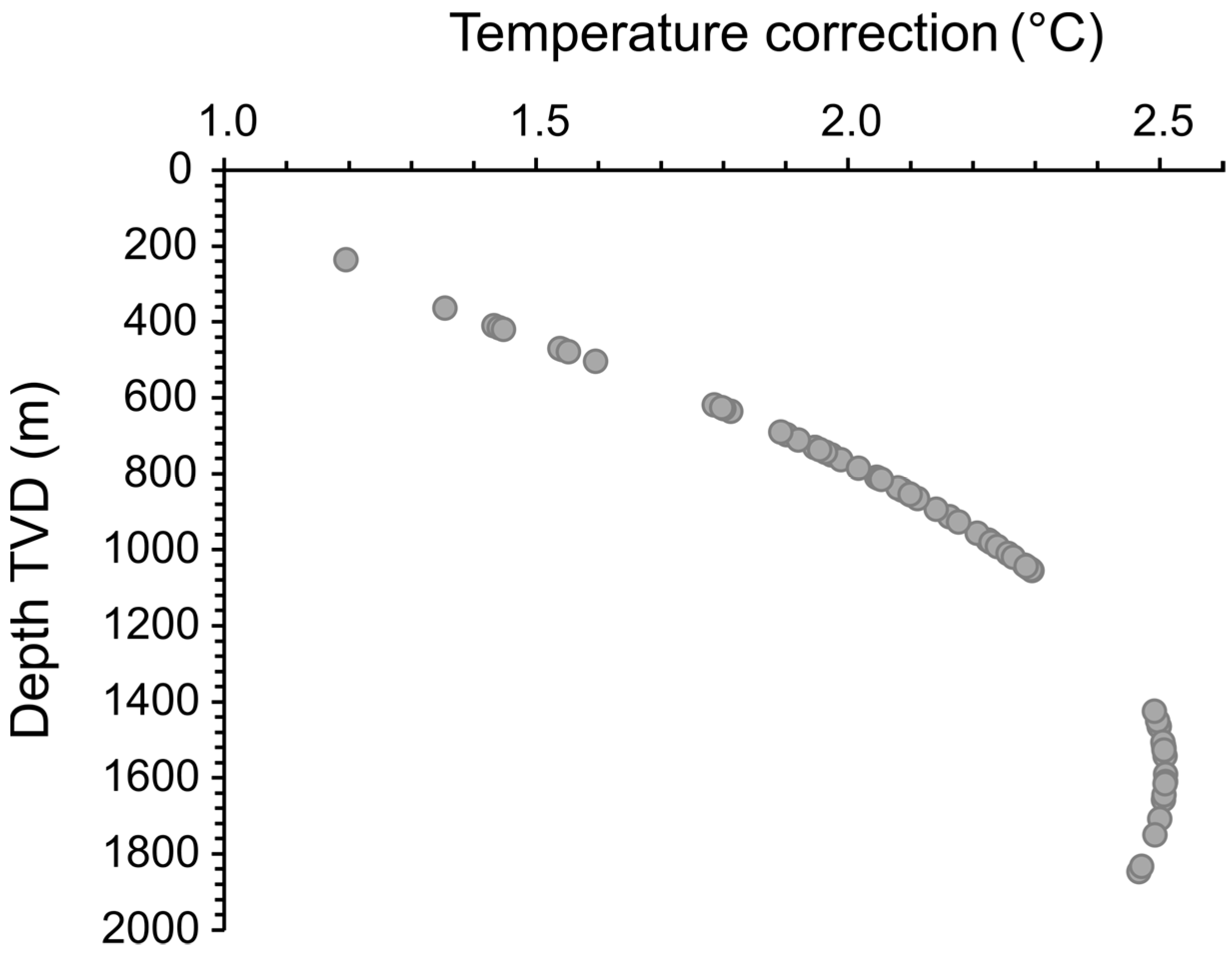
4.2. Paleoclimate Correction

Quaternary glaciation periods are expected to have disturbed the subsurface temperature in the South Slave Region as paleoclimate perturbations were recorded in the temperature signal of deep boreholes over more than 3 km in depth in other nearby regions of Canada (e.g., [4,61,62,63]). BHT and DST temperatures are assumed to have recorded significant Holocene and Pleistocene climatic perturbations. Based on the ground temperature history and the method of Birch [64], the temperature during the Pleistocene glacial cycles in Canada has been considered to be 5 °C colder during the glaciations [1,65]. At the beginning and end of each glaciation, this is the magnitude of temperature change or the temperature step (Ti) that was assumed for the ground surface below the ice sheets ([1]; Figure 5).

The temperature at any depth corrected for paleoclimate effects is (e.g., Jessop [1]) as follows:

$$T_c=T_m+{\sum }_i\left(T_i\right)\left[erf\left({\displaystyle \frac{z}{2\sqrt{\alpha t_1}}}\right)-erf\left({\displaystyle \frac{z}{2\sqrt{\alpha t_2}}}\right)\right]$$

(7)

where T_c (°C) is the temperature corrected for paleoclimate, T_m (°C) is the temperature measured at a certain depth, T_i (°C) is the temperature step between glaciations, erf is the error function, α (m² s⁻¹) is the rock thermal diffusivity (estimated to be ~1.44 × 10⁻⁶ considering the laboratory and thermostratigraphic assessments), t₁ (s) is the end of the ice age, t₂ (s) is the beginning of the ice age, and z (m) is the depth of the temperature measurement.

4.3. Geothermal Gradient Calculation

Below each community, the average geothermal gradient g (°C m⁻¹) was calculated from the corrected temperature data of the nearest wells (Figure 3) using the following equation:

$$g={\displaystyle \frac{\mathsf{\Delta }T}{\mathsf{\Delta }z}}={\displaystyle \frac{T_{\mathrm{c}}-T_{\mathrm{s}}}{∆TVD}}$$

(8)

where ΔT (°C) is the difference between the corrected and the undisturbed ground temperature (T_s = 2.1 °C) divided by Δz (m), the true vertical depth difference. Depending on the purpose of the calculation, the corrected temperature can be BHTs corrected for the drilling disturbance and paleoclimates or DSTs corrected for paleoclimates when required.

The geothermal gradient for wells in Cameron Hills was determined from the slope calculation method using the temperature regression line of the measured profile. The average geothermal gradient g is the reverse of the slope.

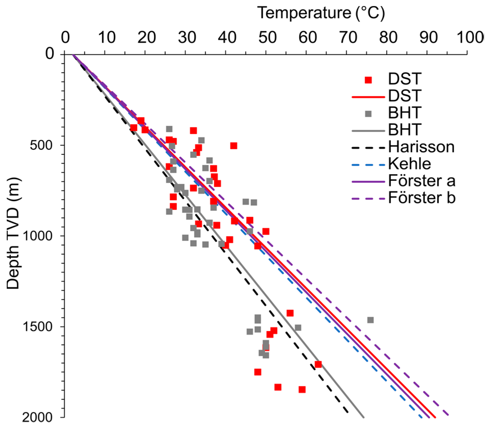
4.4. Verification with Temperature Profiles from Cameron Hills

We used the equilibrium temperature profiles collected from the six wells in Cameron Hills to verify our thermostratigraphic model (Table 3 and Figure 4). This verified approach was then used to evaluate the heat flow (Q₀, W m⁻²) and to predict the temperature below the four South Slave communities where there are no equilibrium temperature profiles available. The heat flow at Cameron Hills was first calculated considering the equilibrium temperature at the bottom of the well. Then, temperature profiles recorded at the six Cameron Hills wells were recalculated according to the thermostratigraphic assessment made in South Slave communities. This temperature–depth model was developed to verify if the selected thermal properties for the geological formations are appropriate for the computed temperature to reproduce the observed temperature. The measured equilibrium temperature at the wells in Cameron Hills is perturbed by paleoclimate effects. Therefore, in this case, no paleoclimate correction was made to predict the ground temperature.

4.4.1. Heat Flow Evaluation for Cameron Hills

Equation (9) (e.g., [45,46,49]) was used to calculate the surface heat flow Q₀ for the wells in Cameron Hills:

$$Q_0=\lambda g+A{\displaystyle \frac{z}{2}}$$

(9)

where the thermal conductivity λ (W m⁻¹ K⁻¹) is the weighted harmonic mean calculated from the lithological units, A (W m⁻³) is the weighted arithmetic average heat generation in the sedimentary rock cover, z (m) is the thickness between the ground surface and measured temperature at both ends of the temperature profile, and g (°C m⁻¹) is the geothermal gradient identified previously.

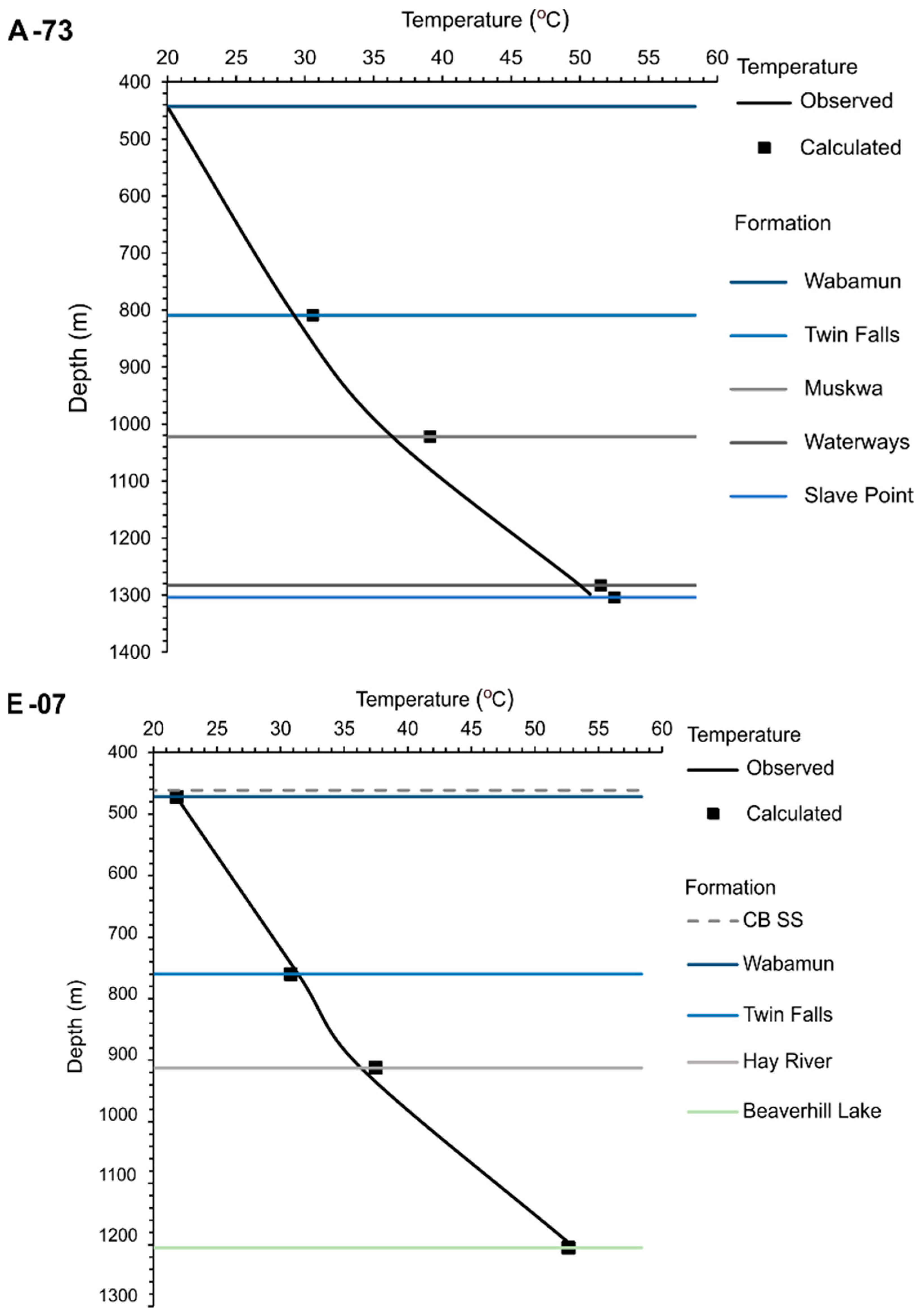
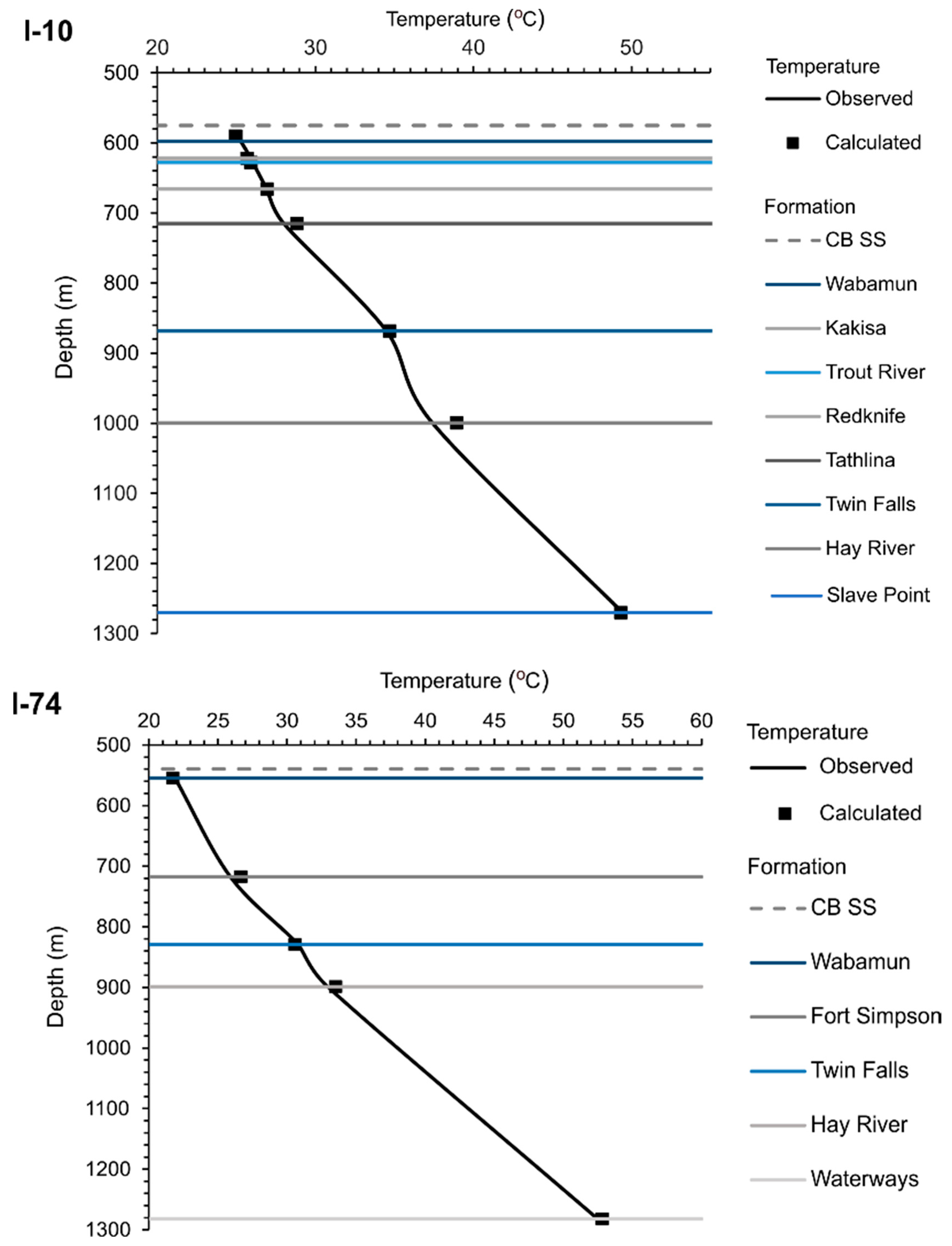
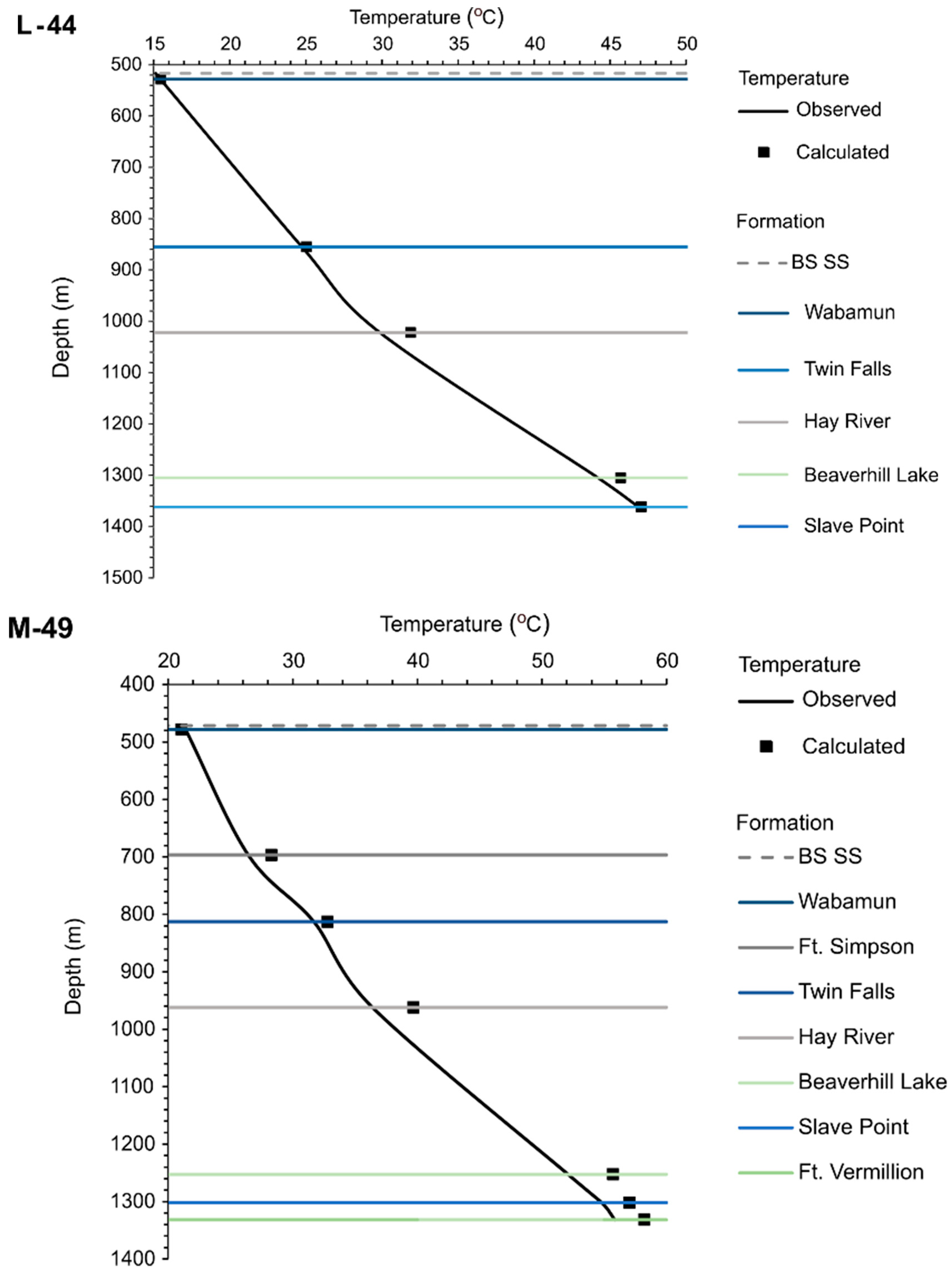
4.4.2. Temperature–Depth Models for Cameron Hills

The 1D calculation was made considering conductive heat transfer in steady-state conditions following (e.g., [1,66,67]):

$$T_{\mathrm{z}}=T_{\mathrm{s}}+{\displaystyle \frac{Q_0 z}{\lambda }}-A{\displaystyle \frac{z^2}{2\mathsf{\lambda }}}$$

(10)

where T_z is the temperature at the depth z (m) in the sedimentary rock formations. Q₀ (W m⁻²) was determined in the previous step and used as boundary conditions.

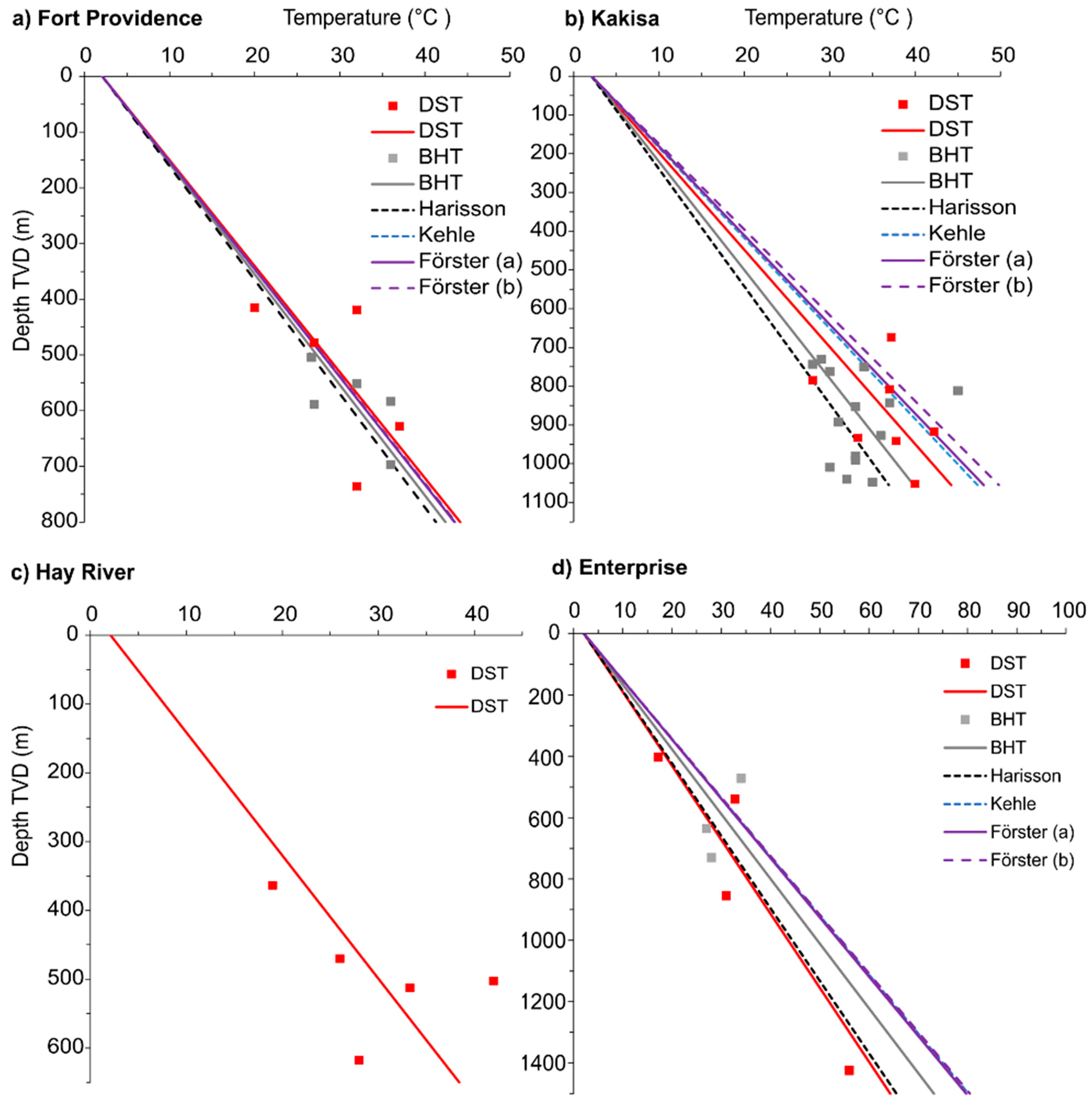
4.5. Prediction of Temperature Profiles for South Slave Communities

After verifying that our thermal conductivity assessment could accurately evaluate the temperature at a certain depth for Cameron Hills, the same approach was used to predict the temperature below the South Slave communities where no equilibrium temperature profile exists.

4.5.1. Heat Flow Evaluation for South Slave Communities

The surface heat flow Q₀ at the location of each community was then calculated using Equation (9). The stratigraphic column thickness z (m) was calculated from the surface to the top of the basement.

4.5.2. Temperature–Depth Model

One-dimensional temperature profiles below the four South Slave communities were calculated using Equation (10), and thermal conductivity was validated with the data from Cameron Hills wells. The temperature profiles predicted in the sedimentary rock cover overlying the crystalline basement assume steady-state conductive heat transfer and consider internal heat generation at the location of the communities. The boundary conditions are the undisturbed ground temperature (T_s = 2.1 °C) and the surface heat flow Q₀.

The paleoclimate correction was not applied to the ground temperature calculation as it reflects the temperature that can be measured in sedimentary rocks below the South Slave communities. Thus, the predicted temperature is perturbed by paleoclimates, as can be expected when measurements are taken at depths of less than a kilometer.

5. Results

5.1. Corrected BHTs

Six of the forty-two BHTs were not corrected because the temperature was recorded at a depth of less than 600 m. The Förster (a) correction revealed corrected BHTs closer to DST temperatures and a smaller standard deviation when compared to other correction methods (Figure 6). The correction factor T_cf (°C) obtained with the Förster (a) method varied from 3.8 °C to 16.2 °C, resulting in corrected BHTs from 30.6 °C to 89.9 °C from 625.8 m to 1657 m in depth.

Due to the depth for which the correction method was developed, only one of four BHTs in Ft. Providence and two of the three BHTs in Enterprise could be corrected for the drilling disturbances (

Table 4. Temperature corrected for paleoclimates in each community.

		DST (n = 5)	Paleoclimate Ti= −5 °C	BHT (n = 4)	Förster (b)	Paleoclimate Ti = −5 °C
Fort Providence	Min	20.0	21.4	26.7	41.3	43.1
	Max	37.0	38.8	36	41.3	43.1
		DST (n = 7)	Paleoclimate Ti = −5 °C	BHT (n=14)	Khele	Paleoclimate Ti = −5 °C
Kakisa	Min	28.0	30.0	28.0	33.2	35.2
	Max	42.2	44.3	45.0	50.7	52.8
		DST (n = 5)	Paleoclimate Ti = −5 °C	BHT (n = 0)
Hay River	Min	19.0	20.3
	Max	42.0	43.6
		DST (n = 2)	Paleoclimate Ti = −5 °C	BHT (n = 3)	Harisson	Paleoclimate Ti = −5 °C
Enterprise	Min	17.2	18.6	27.0	23.6	25.5
	Max	56.0	58.5	34.0	21.2	22.9

n = number of temperature measurements.

). Nevertheless, the uncorrected BHTs above the minimum correction depth were kept to calculate the average geothermal gradient since measurements are relatively shallow and drilling disturbances are expected to be less important. Only DST temperatures were available for Hay River.

The most accurate correction method when analyzing each community individually is Förster (b) in Ft. Providence and Khele in Kakisa. The Harisson method provided a better correlation with DST temperatures in Enterprise (Figure 7). It should be noted that the Harisson correction lowers the corrected temperature when the depth is less than 1000 m. The corresponding corrected temperature range is given in Table 4.

5.2. Paleoclimate Correction

The temperature correction varies between 1.1 °C and 2.5 °C from a depth of 364 m to 1846 m (Figure 8). The temperature ranges for each community are presented in Table 4.

5.3. Geothermal Gradient

The geothermal gradients calculated from the BHTs recorded in 42 wells are 27.6 °C km⁻¹ to 55.1 °C km⁻¹, with a mean of 36.1 ± 7.7 °C km⁻¹. After the drilling correction, the range of geothermal gradients is 35.4 °C/km to 62.6 °C km⁻¹, with an average of 44.3 ± 7.2 °C km⁻¹. The paleoclimate correction of DST temperatures and corrected BHTs revealed an average geothermal gradient of 45.6 ± 12.8 °C km⁻¹and 46.4 ± 7.5 °C km⁻¹, respectively (

Table 5. Geothermal gradient (°C km⁻¹) in the South Slave Region.

	DST (n = 33)	Paleoclimate Ti = −5 °C	BHT (n = 42)	Förster (a)	Paleoclimate Ti = −5 °C
Min	26.2	27.7	27.6	35.4	37.8
Mean	43.1	45.6	36.1	44.2	46.4
Max	79.4	82.5	55.1	62.6	65.1
St.Dev.	12.3	12.8	7.7	7.2	7.5

n = number of temperatures.

).

The temperature gradients are summarized for each community. After applying the paleoclimate correction, the most reliable estimate of the geothermal gradient under Ft. Providence was determined from DST temperatures, which was 55.7 ± 12.3 °C km⁻¹. Despite the fact that the number of BHTs was the same as the number of DST temperatures, only one of the four BHT data points was deep enough to be corrected and resulted in a lower geothermal gradient of 54.8 ± 6.4 °C km⁻¹. In Kakisa, twice as many BHTs were available than DSTs; these corrected BHTs provided the most reliable estimate of the geothermal gradient of 45.2 ± 6.6 °C km⁻¹. Hay River showed the highest mean geothermal gradient of 59.1 ± 14.9 °C km⁻¹, calculated from DST temperatures only. In Enterprise, the most reliable estimate for the geothermal gradient of 44.1 ± 10.6 °C km⁻¹ was obtained from the corrected DST temperatures. Despite the fact that the corrected BHTs resulted in higher values, only two of the three BHTs could be corrected for drilling disturbances due to their shallow depth, and the shallow uncorrected temperatures were kept for paleoclimate correction (

Table 6. Geothermal gradient g (°C km⁻¹) in each community.

		DST (n = 4)	Paleoclimate Ti = −5 °C	BHT (n = 5)	Forster (b)	Paleoclimate Ti = −5 °C
	Min	40.6	43.3	42.3	42.3	45.2
Fort Providence	Mean	52.6	55.7	50.4	51.9	54.8
	Max	71.3	74.8	58.1	58.1	61.0
	St.Dev	12.2	12.3	6.0	6.4	6.4
		DST (n = 7)	Paleoclimate Ti = −5 °C	BHT (n = 14)	Khele	Paleoclimate Ti = −5 °C
	Min	33.0	35.6	27.6	34.8	37.0
Kakisa	Mean	39.9	42.6	35.8	42.8	45.2
	Max	60.9	35.6	52.9	59.9	62.4
	St.Dev	6.9	7.0	6.6	6.5	6.6
		DST (n = 5)	Paleoclimate Ti = −5 °C	BHT (n = 0)
	Min	41.9	44.8
Hay River	Mean	55.9	59.1
	Max	79.4	82.5
	St.Dev	14.9	14.9
		DST (n = 4)	Paleoclimate Ti = −5 °C	BHT (n = 3)	Harisson	Paleoclimate Ti = −5 °C
	Min	33.8	36.2	35.5	29.4	32.8
Enterprise	Mean	41.5	44.1	47.4	42.3	45.7
	Max	56.8	59.8	67.5	67.5	70.8
	St.Dev	10.4	10.6	17.5	21.8	20.8

n = number of temperature measurements. The most reliable estimate of the geothermal gradient is shown in bold.

and Figure 9).

The average geothermal gradient measured, which was affected by the glaciations, in the six wells in Cameron Hills ranges from 35.4 °C km⁻¹ to 43.7 °C km⁻¹, and the paleoclimate correction increases the geothermal gradient from 36.4 °C km⁻¹to 44.6 °C km⁻¹ (

Table 7. Geothermal gradient g (°C km⁻¹) from wells in Cameron Hills.

Well’s Short Name	Measured Gradient	Gradient Paleoclimate Ti = −5 °C
	[°C km−1]	[°C km−1]
A-73	39.2	40.2
E-07	43.7	44.6
I-10	35.4	36.4
I-74	42.5	43.5
L-44	37.8	38.8
M-49	43.5	45.3

).

5.4. Verification with Temperature Profiles from Cameron Hills

5.4.1. Heat Flow Evaluation for Cameron Hills

Table 8. Surface heat flow from wells in Cameron Hills.

Well’s Short Name	Qo	Qo Paleoclimate Ti = −5 °C
	[mW m−2]	[mW m−2]
A-73	104.1	106.8
E07	113.8	116.0
I-10	80.6	83.0
I-74	105.7	108.3
L-44	102.5	105.1
M-49	115.8	120.6

shows the evaluation of the heat flow considering the thermal conductivity in Table 3. The heat flow ranges from 80.6 mW m⁻² to 115.8 mW m⁻², and the paleoclimate correction increased the range from 83.0 mW m⁻² to 120.6 mW m⁻².

5.4.2. Temperature–Depth Model

The calculated temperature is compared to the measured temperature in Cameron Hills (Figure 10). The maximum difference is 3.6 °C. The thermal conductivity assigned to the formations in Cameron Hills seems logical and allows for observed temperatures to be reproduced.

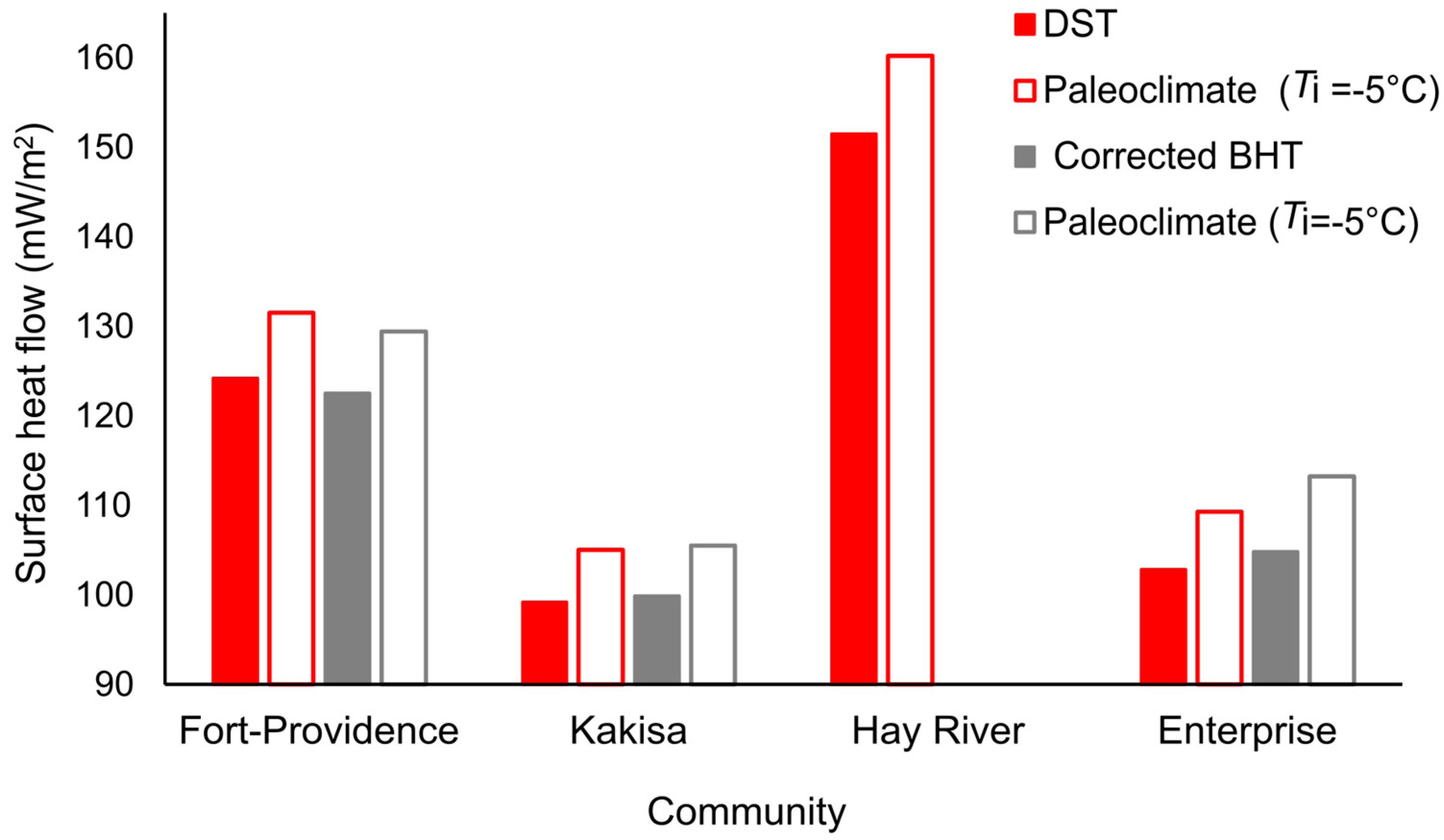
5.5. Prediction of Temperature Profiles for South Slave Communities

5.5.1. Heat Flow Evaluation for South Slave Communities

At the community level, the most logical estimation of the heat flow was determined from the most reliable estimate of the geothermal gradient presented in Section 4.3 (Table 5). Heat flow assessments are either based on DSTs or BHTs corrected for drilling disturbances, and both temperature data were corrected for paleoclimate effects. The estimate of the surface heat flow is 131.5 mW m⁻² in Ft. Providence, 105.5 mW m⁻² in Kakisa, 160.2 mW m⁻² in Hay River, and 109.3 mW m⁻² in Enterprise (Figure 11).

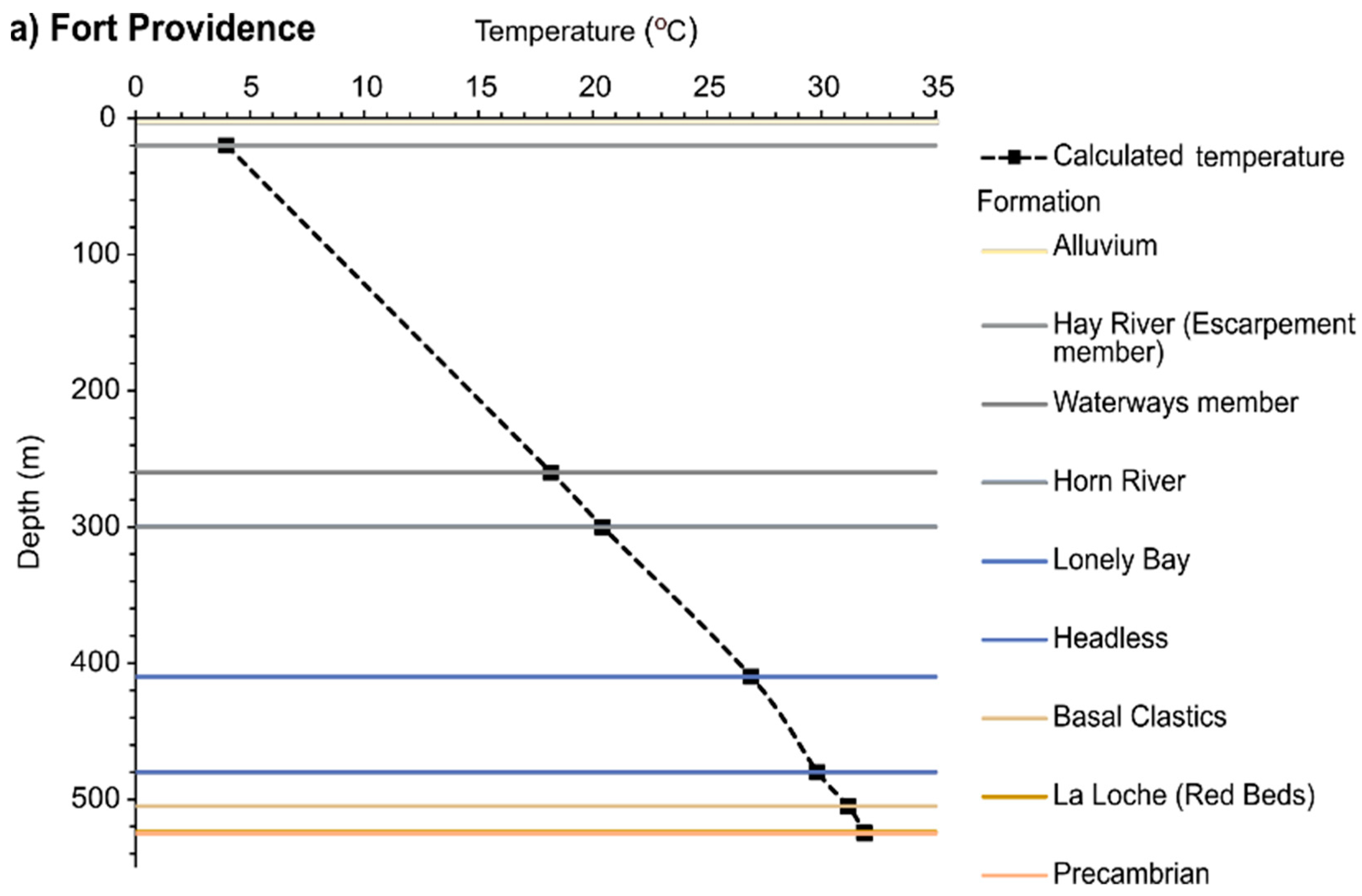
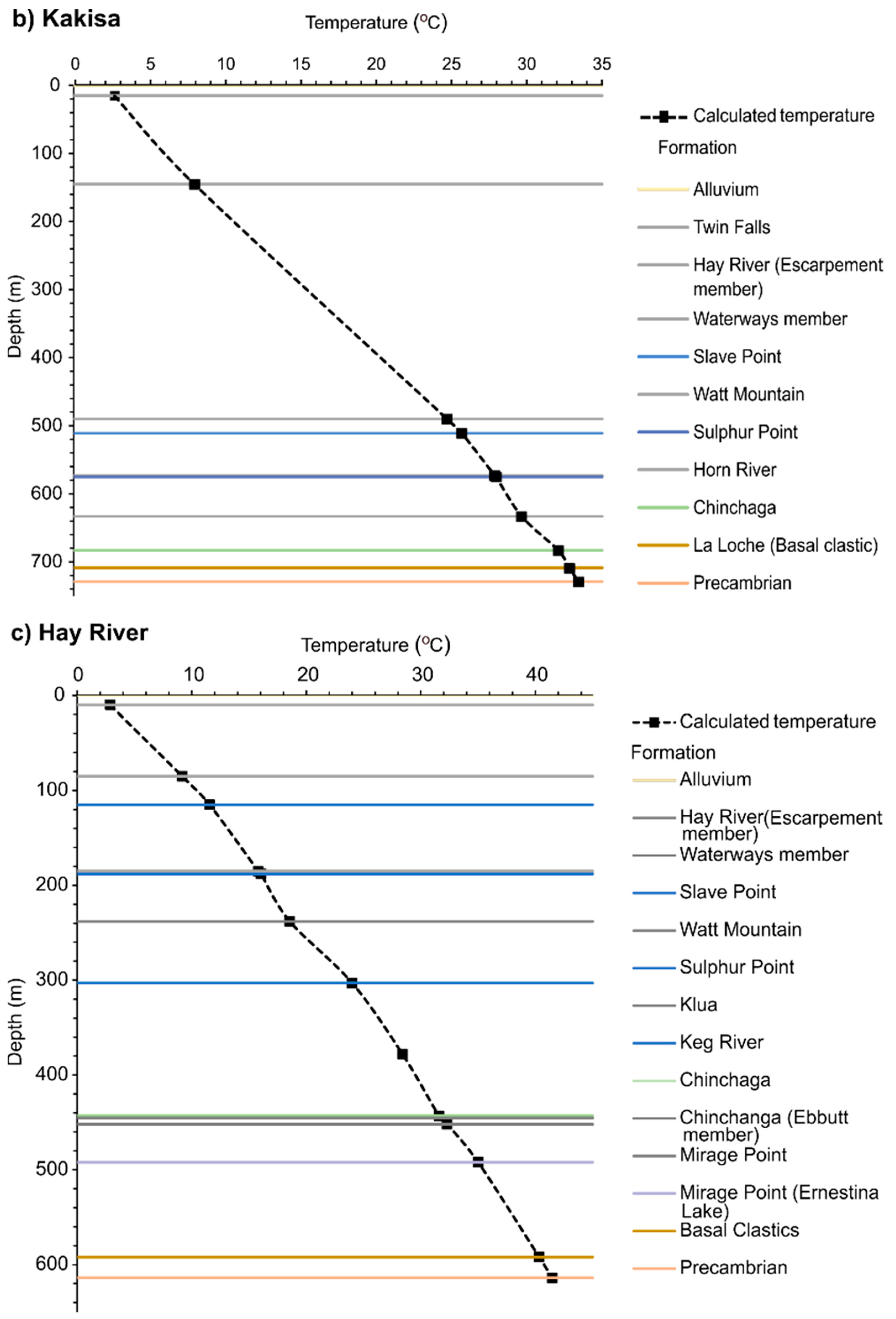
5.5.2. Temperature–Depth Model

For all the communities, the temperature varies from ~3.2 °C under the Quaternary cover to 33.3 °C at the basement top, with a maximum of 36.5 °C in Hay River, where the basement top is at a depth of 614 m. The temperature profiles for Fort Providence, Kakisa, and Enterprise are similar to each other due to the thick shale formations underlying the communities. The maximum temperature reached for these communities is 33.1 °C at the top of the crystalline basement (Figure 12).

6. Discussion

The analyses of BHT and DST data (75 readings) from the South Slave Region yielded a local geothermal gradient varying from 45.2 ± 6.6 °C km⁻¹ to 59.1 ± 14.9 °C km⁻¹ below the communities of Ft. Providence, Kakisa, Hay River, and Enterprise. Heat flow estimates vary from 105.7 mW m⁻² to 160.2 mW m⁻² under these communities. These values are comparable to the heat flow calculated in the Cameron Hills region, where equilibrium temperature profiles were used for verification (Table 8 and Figure 11). The regional temperature distribution throughout the WCSB was previously mapped by other researchers (e.g., [68,69]). High geothermal gradients (>35 °C km⁻¹) were estimated in the NWT, north of a 65° latitude and to the east of the Mackenzie Mountains, with values of 40 °C km⁻¹ to 50 °C km⁻¹ [5]. Our work suggests elevated geothermal gradients and heat flows under four communities in the Southern NWT and confirms the previous elevated geothermal gradient estimates. These results indicate significant geothermal potential in the communities of Ft. Providence and Hay River. The geothermal gradient in Kakisa and Enterprise is expected to be >40 °C km⁻¹, which is highly favorable, but the small population of those communities could be a challenge for the economic exploitation of the geothermal resource.

For this study, no information on the quality of the temperature readings was available since this relates to the flow rate during the DST and the mud circulation time for BHT measurements [5]. Limited temperature data were available for each community as they are located in a remote northern region. The number of temperature data points available in each community was the criterion to determine the most reliable type of data to estimate the geothermal gradient from the group of wells near each community. A large number of BHTs were favored when possible, but the number of DST temperatures was more important for three communities (Ft. Providence, Hay River, and Enterprise).

The measured temperatures from six wells in Cameron Hills were used to verify our thermostratigraphic approach for temperature predictions. A similar approach that uses equilibrium temperature was performed for several basins in the USA (e.g., [26,27]). Majorowicz et al. [70] concluded that even corrected BHTs tend to be systematically higher compared to equilibrium temperature measurements of shallow basins (from 500 to 900 m in depth) for wells in the Rocky Mountain Foothills and at the western edge of the WCSB and that shallow BHTs contain systematic errors. This was also confirmed and discussed by the work of Majorowicz et al. [69], who estimated the geothermal gradient and regionally mapped the geothermal anomalies of the WCSB. The discrepancies between calculated and observed temperatures can be explained by many factors, but the input temperature remains the parameter that has the highest impact on the final geothermal gradient and heat flow estimation [4]. It should also be noted that only Kakisa and Enterprise have temperature data recorded at a depth greater than 1 km (Figure 7), resulting in the two communities having the lowest gradients, but had values comparable to those of Cameron Hills. It is therefore possible that considering data from a shallow depth (e.g., Hay River) resulted in an overestimation of the geothermal gradient.

Our analyses have demonstrated that the temperature predicted below the four communities presents similar trends to that measured for Cameron Hills. The range of thermal conductivity is a source of uncertainty, but verification with temperature profiles in Cameron Hills resulted in small differences of 3.61 °C between calculated and measured temperatures (Figure 10). The radiogenic heat production is part of the assessable intrinsic property of the rock that cannot be ignored in the equation of the heat flow. However, it had a relatively minor impact on the calculation made in this study since the total thickness of the sedimentary rock formations is less than 1 km and the temperature predictions are for a relatively shallow depth. The heat production rate calculated from either the radiogenic element content (determined with inductively coupled plasma techniques) or gamma ray is similar for the geological formations common to the South Slave communities (Table 2) and Cameron Hills (Table 3).

The thermal conductivity is assumed to be uniform in each geological formation and is responsible for changes in the geothermal gradient at geological formation contacts. Lithologies with a lower thermal conductivity show a relatively more rapid increase in temperature with depth (Figure 12). The most prominent lithologies below the South Slave communities are shales and carbonates. Their estimated thermal conductivity is consistent with thermal conductivity of the typical sedimentary rocks in the WCBS and has values ranging from 1.4 ± 0.4 W m⁻¹K⁻¹ to 2.1 ± 0.4 W m⁻¹ K⁻¹ in shale, 2.4 ± 0.9 W m⁻¹ K⁻¹ to 3.4 ± 3.0 Wm⁻¹ K⁻¹ in limestone, 3.1 ± 1.4 W m⁻¹ K⁻¹ to 5.0 ± 0.6 Wm⁻¹K⁻¹ in dolomite, and 2.8 W m⁻¹ K⁻¹ to 4.7 ± 2.8 W m⁻¹ K⁻¹ in sandstone (e.g., [1,71]). The low harmonic average of thermal conductivity estimated for sedimentary rocks below the four communities (~2.5 W m⁻¹ K⁻¹) reveals its blanketing effect and can partially explain the high geothermal gradient given by the significant thickness of shales in this high heat flow region (Figure 4 and Figure 12). Furthermore, the area of interest is located at the edge of the platform where major faults and shear zones affected the basement in an extensional tectonic regime (Figure 3). Majorowicz [72] proposed that this heat flow anomaly is due to an increased mantle upflow beneath the region, coinciding with crustal faults such as the Great Slave Lake shear zone that separates the Churchill and Slave Provinces and potentially continues under the sedimentary basin (e.g., [73,74] and Figure 3).

This study improved the geothermal knowledge of the South Slave Region by using recently acquired information on thermal properties to evaluate the heat flow and interpolate the subsurface temperature from the surface to the top of the crystalline basement. The regional and deep basement faults that cross the communities (Figure 2) could have an influence on the permeability and convective heat transfer. However, an analysis of the structural context was not addressed in this study. Natural hydrothermal systems are commonly present in fractured rocks and typically associated with extensional faulting (e.g., [75,76,77]). This is a limitation of our study because we only focused on conductive heat transfer mechanisms.

7. Conclusions

A compilation of DST temperatures and BHTs that were corrected for drilling disturbances allowed the evaluation of the geothermal gradient and heat flow below communities of the South Slave Region to subsequently predict the temperature–depth distribution in the sedimentary basin formations. The current estimation of the geothermal gradient is >40 °C km⁻¹ and up to 100 mW m⁻² for heat flow.

The results indicate a high geothermal gradient and high surface heat flow suitable for the direct use of geothermal resources at the depth of sedimentary rock formations according to the Lindal diagram [78]. The communities, particularly Hay River, could potentially exploit the geothermal resource. Here, the high geothermal gradient could facilitate exploitation at a shallow drilling depth and result in projects that may be economically beneficial.

Based on these models, the heat flow in the South Slave Region would be the highest one in the entire WCSB, but geothermal exploration boreholes will have to be drilled to confirm these results. Drilling exploration wells and measuring equilibrium temperature profiles are the next steps to confirm our findings and eventually exploit geothermal resources. The use of thermally equilibrated temperature measurement data from wells in Cameron Hills allowed the verification of our model to determine if the thermal conductivities assigned to the geological formations underlying the South Slave communities are logical, using formations common to both areas (Twin Falls, Hay River, and Slave Point formations). The thermal conductivity values of the sedimentary rocks vary from 1.4 W m−1 K⁻¹ to 3.5 W m−1 K⁻¹. However, the nature and thermal properties of the Precambrian basement below the sedimentary basin at the location of the South Slave communities need to be defined in future work in order to extrapolate the temperature at depth below the basin. Evaluating the thermal conductivity of the crystalline basement will be crucial for obtaining a reliable estimate of temperature in deep basement rocks.

In the Northwest Territories, other communities like Fort Simpson, Jean Marie River, Nahanni Butte, and Fort Liard also have a high geothermal potential and are situated in a similar geological setting. The methodology presented in this article could be applied for a better evaluation of the geothermal potential at these locations.

References

1. Jessop, A.M. Chapter 3—Analysis and Correction of Heat Flow on Land. In Developments in Solid Earth Geophysics; Jessop, A.M., Ed.; Elsevier: Amsterdam, The Netherlands, 1990; Volume 17, pp. 57–85. [Google Scholar] [CrossRef]
2. Majorowicz, J.; Šafanda, J.; Torun-1 Working Group. Heat flow variation with depth in Poland: Evidence from equilibrium temperature logs in 2.9-km-deep well Torun-1. Int. J. Earth Sci. 2008, 97, 307–315. [Google Scholar] [CrossRef]
3. Augustine, C.; Tester, J.W.; Anderson, B.; Petty, S.; Livesay, B. A comparison of geothermal with oil and gas well drilling costs. In Proceedings of the 31st Workshop on Geothermal Reservoir Engineering, Stanford, CA, USA, 30 February 2006. [Google Scholar]
4. Bédard, K.; Comeau, F.-A.; Raymond, J.; Malo, M.; Nasr, M. Geothermal Characterization of the St. Lawrence Lowlands Sedimentary Basin, Québec, Canada. Nat. Resour. Res. 2018, 27, 479–502. [Google Scholar] [CrossRef]
5. Grasby, S.; Majorowicz, J.; McCune, G. Geothermal Energy Potential for Northern Communities Open File; Report No: 7350; Her Majesty the Queen in Right of Canada: Ottawa, ON, USA, 2013. [Google Scholar]
6. Harrison, W.E.; Luza, K.V.; Prater, M.L.; Reddr, R.J. Geothermal Resource Assessment in Oklahoma Special Paper; Report No: DE-AS07-80ID12172; Oklahoma Geological Survey: Norman, OK, USA, 1983. [Google Scholar]
7. Majorowicz, J.; Grasby, S.E. Deep Geothermal Heating Potential for the Communities of the Western Canadian Sedimentary Basin. Energies 2021, 14, 706. [Google Scholar] [CrossRef]
8. Grasby, S.; Majorowicz, J.; Fiess, K. Geothermal Energy Potential of Northwest Territories, Canada. In Proceedings of the World Geothermal Congress 2020+1, Reykjavik, Iceland, 24–27 October 2021. [Google Scholar]
9. Grasby, S.E.; Allen, D.M.; Bell, S.; Chen, Z.; Ferguson, G.; Jessop, A.; Kelman, M.; Majorowicz, M.; Ko, J.; Moore, M.; et al. Geothermal Energy Resource Potential of Canada Open File (Revised); Report No: 6914.; Natural Resources Canada: Ottawa, ON, Canada, 2011. [Google Scholar]
10. EBA Engineering Consultants Ltd. Geothermal Favourability Map Northwest Territories Report 2010; Report No: Y22101146; Northwest Territories Environment and Natural Resources: Yellowknife, NT, Canada, 2010. [Google Scholar]
11. Petrel Robertson Consulting Ltd. Geothermal Database Compilation Internal Report; Petrel Robertson Consulting Ltd.: Calgary, AB, Canada, 2022. [Google Scholar]
12. OROGO(2022) Well Status files. Office of the Regulator of Oil and Gas Operations. Available online: https://www.orogo.gov.nt.ca/en/resources-0 (accessed on 19 January 2022).
13. Smejkal, E.J.; Hickson, C.J.; Collard, J. Revisiting the geothermal potential of the Dehcho Region in NWT: New data from old wells. In Proceedings of the Geoconvention, Calgary, AB, Canada, 15–17 May 2023. [Google Scholar]
14. Davenport, P.H. Exploration Areas of the NWT, Yukon and Nunavut; ESRI ArcView® GIS Shapefiles; Geological Survey of Canada: Calgary, AB, Canada, 2001. [Google Scholar]
15. Rocheleau, J.; Fiess, K.M. Northwest Territories Oil and Gas Poster Series: Basins & Petroleum Resources, Table of Formations, Schematic Cross Sections Open File. Report No: 2014-03. 2014. Available online: https://www.nwtgeoscience.ca/sites/ntgs/files/content/table_of_formations_2014_0.pdf (accessed on 23 March 2024).
16. Carvalho, H.D.S.; Vacquier, V.D. Method for determining terrestrial heat flow in oil fields. Geophysics 1977, 42, 584–593. [Google Scholar] [CrossRef]
17. Majorowicz, J.M.; Jessop, A.M. Canadian Sedimentary Basin. Tectonophysics 1981, 74, 209–238. [Google Scholar] [CrossRef]
18. Reiter, M.; Jessop, A.M. Estimates of terrestrial heat flow in offshore eastern Canada. Can. J. Earth Sci. 1985, 22, 1503–1517. [Google Scholar] [CrossRef]
19. Kenneth, E.P.; Philip, H.N. Criteria to Determine Borehole Formation Temperatures for Calibration of Basin and Petroleum System Models. In Proceedings of the AAPG Annual Convention and Exhibition, Denver, CO, USA, 7–10 June 2009. [Google Scholar]
20. Deming, D.; Chapman, D.S. Heat Flow in the Utah-Wyoming Thrust Belt From Analysis of Bottom-Hole Temperature Data Measured in Oil and Gas Wells. J. Geophys. Res. Solid Earth 1988, 93, 13657–13672. [Google Scholar] [CrossRef]
21. Dowdle, W.L.; Cobb, W.M. Static Formation Temperature From Well Logs—An Empirical Method. J. Pet. Technol. 1975, 27, 1326–1330. [Google Scholar] [CrossRef]
22. Förster, A.; Merriam, D.; Davis, J. Spatial analysis of temperature (BHT/DST) data and consequences for heat-flow determination in sedimentary basins. Int. J. Earth Sci. 1997, 86, 252–261. [Google Scholar] [CrossRef]
23. Blackwell, D.D.; Richards, M. Geothermal Map of North America. AAPG Map, scale Calibration of the AAPG Geothermal Survey of North America BHT data base. In Proceedings of the AAPG Annual Meeting, Poster Session, Dallas, TX, USA, 18–21 April 2004. [Google Scholar]
24. Blackwell, D.D.; Richards, M.; Stepp, P. Texas Geothermal Assessment for the I35 Corridor East Final Report; Report No: CM709; SMU Geothermal Laboratory: Dallas, TX, USA, 2010. [Google Scholar]
25. Kehle, R.O.; Schoeppel, R.J.; Deford, R.K. The AAPG geothermal survey of North America. Geothermics 1970, 2, 358–367. [Google Scholar] [CrossRef]
26. Crowell, A.M.; Ochsner, A.T.; Gosnold, W. Correcting Bottom-Hole Temperatures in the Denver Basin: Colorado and Nebraska. In Proceedings of the Geothermal Resources Council Annual Meeting 2012, Reno, NV, USA, 30 September–3 October 2012. [Google Scholar]
27. Crowell, A.; Gosnold, W. Correcting Bottom Hole Temperatures: A Look at the Permian Basin (Texas), Williston Basin (North Dakota), Anadarko and Arkoma Basins (Oklahoma). In Proceedings of the Geothermal Resources Council Annual Meeting 2011, San Diego, CA, USA, 23–26 October.2011. [Google Scholar]
28. Westaway, R.; Younger, P.L. Accounting for palaeoclimate and topography: A rigorous approach to correction of the British geothermal dataset. Geothermics 2013, 48, 31–51. [Google Scholar] [CrossRef]
29. Dyke, A.S. An outline of North American deglaciation with emphasis on central and northern Canada. In Developments in Quaternary Sciences; Ehlers, J., Gibbard, P.L., Eds.; Elsevier: Amsterdam, The Netherlands, 2004; Volume 2, pp. 373–424. [Google Scholar] [CrossRef]
30. Lemmen, D.S.; Duk-Rodkin, A.; Bednarski, J.M. Late glacial drainage systems along the northwestern margin of the Laurentide Ice Sheet. Quat. Sci. Rev. 1994, 13, 805–828. [Google Scholar] [CrossRef]
31. Stott, D.F.; Klassen, R.W. Geomorphic divisions. In Sedimentary Cover of the Craton in Canada; Stott, D.F., Aitken, J.D., Eds.; Geological Survey of Canada, Geology of Canada: Ottawa, ON, Canada, 1993; Volume 5, pp. 31–44. [Google Scholar]
32. Meijer Drees, N.C. The Devonian Succession in the Subsurface of the Great Slave and Great Bear Plains, Northwest Territories; Geological Survey of Canada: Ottawa, ON, Canada, 1993; p. 231. [Google Scholar] [CrossRef]
33. Moore, P.F. Devonian. In Sedimentary Cover of the Craton in Canada; Stott, D.F., Aitken, J.D., Eds.; Geological Survey of Canada, Geology of Canada: Ottawa, ON, Canada, 1993; Volume 5, pp. 150–201. [Google Scholar]
34. Morrow, D.W.; Geldsetzer, H.H.J. Devonian of the eastern Canadian Cordillera. In Devonian of the World Regional Syntheses; McMillan, N.J., Embry, A.F., Glass, D.J., Eds.; Canadian Society of Petroleum Geologists: Calgary, Canada, 1988; Volume 1, pp. 85–121. [Google Scholar]
35. Mossop, G.; Shetsen, I. Geological Atlas of the Western Canada Sedimentary Basin. 1994. Available online: https://ags.aer.ca/reports/atlas-western-canada-sedimentary-basin (accessed on 12 January 2022).
36. Gal, L.P.; Jones, A.L. Evaluation of oil and gas potential in the Deh Cho territory Open File; 2003. Report No: 2003-03.
37. Wright, G.; McMechan, M.; Potter, D. Structure and architecture of the Western Canada sedimentary basin. In Geological atlas of the Western Canada Sedimentary Basin; Mossop, G., Dixon, J., Eds.; Canadian Society of Petroleum Geologists and Alberta Research Council: Calgary, Canada, 1994; Volume 4, pp. 25–40. [Google Scholar]
38. Smith, I.R.; Christine, D.; Grant, H.; Roger, C.P. A drift isopach model for the southwestern Great Slave Lake region, Northwest Territories, Canada. J. Maps 2023, 19, 2147871. [Google Scholar] [CrossRef]
39. Morrow, D.W.; MacLean, B.C.; Tzeng, P.; Pana, D. Subsurface Paleozoic Structure and Isopach Maps and Selected Seismic Lines in Southern Northwest Territories and Northern Alberta: Implications for Mineral and Petroleum Potential Open File; Report No: 4366; Geological Survey of Canada: Calgary, Canada, 2002. [Google Scholar]
40. Northwest Territories Geological Survey (2023) Geology Map. Available online: https://ntgs-open-data-ntgs.hub.arcgis.com/ (accessed on 2 August 2022).
41. Ouzzane, M.; Eslami-nejad, P.; Badache, M.; Aidoun, Z. New correlations for the prediction of the undisturbed ground temperature. Geothermics 2015, 53, 379–384. [Google Scholar] [CrossRef]
42. Environment and Climate Change Canada (2019) Historical Climate Data. Canada: Government of Canada. Available online: http://climate.weather.gc.ca/ (accessed on 20 April 2023).
43. Rajaobelison, M.; Thibault, M.; Comeau, F.-A.; Raymond, J.; Terlaky, V. Laboratory analyses on split core samples from wells to assess the geothermal potential of the South Slave Region, Northwest Territories; Report No: OR 2023-015. Can. Open Rep. 2023, in press. [Google Scholar]
44. Clauser, C. Thermal Storage and Transport Properties of Rocks, I: Heat Capacity and Latent Heat. In Encyclopedia of Solid Earth Geophysics; Gupta, H.K., Ed.; Springer: Dordrecht, The Netherlands, 2011; pp. 1423–1431. [Google Scholar] [CrossRef]
45. Beardsmore, G.; Cull, J. Crustal Heat Flow: A guide to Measurement and Modelling, 1st ed.; Cambridge University Press: New York, NY, USA, 2001; p. 324. [Google Scholar] [CrossRef]
46. Jaupart, C.; Mareschal, J.-C. Heat Generation and Transport in the Earth; Cambridge University Press: New York, NY, USA, 2010; p. 462. [Google Scholar]
47. Popov, Y.A.; Beardsmore, G.; Clauser, C.; Roy, S. ISRM suggested methods for determining thermal properties of rocks from laboratory tests at atmospheric pressure. Rock Mech. Rock Eng. 2016, 49, 4179–4207. [Google Scholar] [CrossRef]
48. Clauser, C.; Huenges, E. Thermal conductivity of rocks and minerals. In Rock Physics and Phase Relations; Ahrens, T.J., Ed.; AGU Reference Shelf 3: Washington, DC, USA, 1995; pp. 105–126. [Google Scholar] [CrossRef]
49. Eppelbaum, L.; Kutasov, I.; Pilchin, A. Applied Geothermics, ed.; Springer: Heidelberg, Germany; New York, NY, USA; Dordrecht, The Netherlnds; London, UK, 2014; p. 757. [Google Scholar] [CrossRef]
50. Larmagnat, S.; Lavoie, D.; Rajaobelison, M.M.; Raymond, J. Geothermal Assessment of a Conventional Hydrocarbon Reservoir in Eastern Québec: Preliminary Field and Petrophysical Data Open File; Report No: 8597; Geological Survey of Canada, Geology of Canada: Ottawa, ON, Canada, 2019. [Google Scholar]
51. Mielke, P.; Bär, K.; Sass, I. Determining the relationship of thermal conductivity and compressional wave velocity of common rock types as a basis for reservoir characterization. J. Appl. Geophys. 2017, 140, 135–144. [Google Scholar] [CrossRef]
52. Tang, B.; Zhu, C.; Xu, M.; Chen, T.; Hu, S. Thermal conductivity of sedimentary rocks in the Sichuan basin, Southwest China. Energy Explor. Exploit. 2018, 37, 691–720. [Google Scholar] [CrossRef]
53. Cermak, V.; Rybach, L. Thermal Conductivity and Specific Heat of Minerals and Rocks. In Physical Properties of Rocks · SubVolume A; Angenheister, G., Ed.; Springer: Berlin/Heidelberg, Germany; New York, NY, USA, 1982; Volume 1A, pp. 305–343. [Google Scholar] [CrossRef]
54. Pasquale, V.; Verdoya, M.; Chiozzi, P. Measurements of rock thermal conductivity with a Transient Divided Bar. Geothermics 2015, 53, 183–189. [Google Scholar] [CrossRef]
55. Bücker, C.; Rybach, L. A simple method to determine heat production from gamma-ray logs. Mar. Pet. Geol. 1996, 13, 373–375. [Google Scholar] [CrossRef]
56. Hasterok, D.; Gard, M.; Webb, J. On the radiogenic heat production of metamorphic, igneous, and sedimentary rocks. Geosci. Front. 2018, 9, 1777–1794. [Google Scholar] [CrossRef]
57. Waples, D.W. A New Model for Heat Flow in Extensional Basins: Estimating Radiogenic Heat Production. Nat. Resour. Res. 2002, 11, 125–133. [Google Scholar] [CrossRef]
58. Burrus, J.; Foucher, J.P. Contribution to the thermal regime of the Provençal Basin based on Flumed heat flow surveys and previous investigations. Tectonophysics 1986, 128, 303–334. [Google Scholar] [CrossRef]
59. Richards, M.; Crowell, A.M. (SMU Geothermal Laboratory, Dallas, TX, USA). Personal Communication, 2012.
60. Mareschal, J.C.; Jaupart, C. Variations of surface heat flow and lithospheric thermal structure beneath the North American craton. Earth Planet. Sci. Lett. 2004, 223, 65–77. [Google Scholar] [CrossRef]
61. Majorowicz, J.; Gosnold, W.; Gray, A.; Safanda, J.; Klenner, R.; Unsworth, M. Implications of post-glacial warming for northern Alberta heat flow-correcting for the underestimate of the geothermal potential. In Proceedings of the Geothermal Resources Council Annual Meeting 2012, Reno, NV, USA, 30 September–3 October.2012. [Google Scholar]
62. Beltrami, H.; Gosselin, C.; Mareschal, J.-C. Ground surface temperatures in Canada: Spatial and temporal variability. Geophys. Res. Lett. 2003, 30, 1–6. [Google Scholar] [CrossRef]
63. Majorowicz, J.; Chan, J.; Crowell, J.; Gosnold, W.; Heaman, L.M.; Kück, J.; Nieuwenhuis, G.; Schmitt, D.R.; Unsworth, M.; Walsh, N.J.; et al. The first deep heat flow determination in crystalline basement rocks beneath the Western Canadian Sedimentary Basin. Geophys. J. Int. 2014, 197, 731–747. [Google Scholar] [CrossRef]
64. Birch, A.F. The effects of Pleistocene climatic variations upon geothermal gradients. Am. J. Sci. 1948, 246, 729. [Google Scholar] [CrossRef]
65. Jessop, A.M. The Distribution of Glacial Perturbation of Heat Flow in Canada. Can. J. Earth Sci. 1971, 8, 162–166. [Google Scholar] [CrossRef]
66. Stein, C.A. Heat Flow of the Earth. In Global Earth Physics; American Geophysical Union: Washington, DC, USA, 1995; pp. 144–158. [Google Scholar] [CrossRef]
67. Turcotte, D.L.; Schubert, G. Geodynamics, 3rd ed.; Cambridge University Press: New York, NY, USA, 2014; p. 615. [Google Scholar]
68. Majorowicz, J.; Grasby, S.E. Heat flow, depth–temperature variations and stored thermal energy for enhanced geothermal systems in Canada. J. Geophys. Eng. 2010, 7, 232–241. [Google Scholar] [CrossRef]
69. Allan Gray, D.; Majorowicz, J.; Unsworth, M. Investigation of the geothermal state of sedimentary basins using oil industry thermal data: Case study from Northern Alberta exhibiting the need to systematically remove biased data. J. Geophys. Eng. 2012, 9, 534–548. [Google Scholar] [CrossRef]
70. Majorowicz, J.A.; Garven, G.; Jessop, A.; Jessop, C. Present Heat Flow Along a Profile Across the Western Canada Sedimentary Basin: The Extent of Hydrodynamic Influence. In Geothermics in Basin Analysis; Förster, A., Merriam, D.F., Eds.; Springer: Boston, MA, USA, 1999; pp. 61–79. [Google Scholar] [CrossRef]
71. Beach, R.D.W.; Jones, F.W.; Majorowicz, J.A. Heat flow and heat generation estimates for the churchill basement of the western canadian basin in Alberta, Canada. Geothermics 1987, 16, 1–16. [Google Scholar] [CrossRef]
72. Majorowicz, J. Anomalous heat flow regime in the Western margin of the North American Craton, Canada. J. Geodyn. 1996, 21, 123–140. [Google Scholar] [CrossRef]
73. Eaton, D.W.; Hope, J. Structure of the crust and upper mantle of the Great Slave Lake shear zone, northwestern Canada, from teleseismic analysis and gravity modelling1. Can. J. Earth Sci. 2003, 40, 1203–1218. [Google Scholar] [CrossRef]
74. Yin, Y.; Unsworth, M.; Liddell, M.; Pana, D.; Craven, J.A. Electrical resistivity structure of the Great Slave Lake shear zone, northwest Canada: Implications for tectonic history. Geophys. J. Int. 2014, 199, 178–199. [Google Scholar] [CrossRef]
75. Faulds, J.; Coolbaugh, M.; Bouchot, V.; Moeck, I.; Oguz, K. Characterizing structural controls of geothermal reservoirs in the Great Basin, USA, and Western Turkey: Developing successful exploration strategies in extended terranes. Proceedings of World Geothermal Congress, Bali, Indonesia, 25–30 April 2010. [Google Scholar]
76. Moeck, I. A new classification scheme for deep geothermal systems based on geologic controls. In Proceedings of the EGU General Assembly Conference Abstracts, Vienna, Austria, 22–27 April 2012. [Google Scholar]
77. Rajaobelison, M.; Raymond, J.; Malo, M.; Dezayes, C.; Larmagnat, S. Understanding heat transfer along extensional faults: The case of the Ambilobe and Ambanja geothermal systems of Madagascar. Geothermics 2022, 104, 102455. [Google Scholar] [CrossRef]
78. Lindal, B. Industrial and other applications of geothermal energy. Geotherm. Energy Rev. Res. Dev. 1973, 135–148. [Google Scholar]
Figure 1. (a) The location of the study area is outlined in blue. The geological provinces and general simplified tectonic structure lines with the exploration areas are from the base map, modified according to [14,15]. Pink dots indicate the location of wells with subsurface temperature information. The well locations are from the map of Petrel Robertson Consulting Ltd. [11]. (b) Geothermal feasibility map of the Northwest Territories modified from EBA Engineering Consultants Ltd. [10].
Energies 17 04165 g001
Figure 3. Location of the 75 wells with measured DSTs and BHTs. The white boxes delineate the wells selected for each community. The wells with IDs are those in the Cameron Hills region that have equilibrium temperature data. The geological base map was modified from the Northwest Territories Geological Survey [40] and has the same legend as Figure 2.
Energies 17 04165 g003
Figure 4. Thermostratigraphic log at the location of the four South Slave communities, reproduced from Rajaobelison et al. [43].
Energies 17 04165 g004aEnergies 17 04165 g004b
Figure 5. Timeline of Pleistocene and Holocene climate events according to a relative change in temperature of 5 °C, modified from Bédard et al. [4].
Energies 17 04165 g005
Figure 6. Uncorrected BHTs for the South Slave Region showing linear regressions for corrected BHTs using the empirical equations [6,22,25,59], compared to DST temperatures and their trendlines.
Energies 17 04165 g006
Figure 7. Uncorrected BHTs with the regression lines from corrected BHTs using the empirical equations [6,22,25,59] compared to DST temperature trendlines for each community in the South Slave Region.
Energies 17 04165 g007
Figure 8. Paleoclimate temperature correction calculated as a function of the depth at which DSTs and BHTs were measured in the South Slave Region.
Energies 17 04165 g008
Figure 9. Geothermal gradient estimates of the four South Slave communities.
Energies 17 04165 g009
Figure 10. Calculated temperature plotted against observed temperature recorded in the six wells in the Cameron Hills region.
Energies 17 04165 g010aEnergies 17 04165 g010bEnergies 17 04165 g010c
Figure 11. Heat flow estimated for communities in the South Slave Region.
Energies 17 04165 g011
Figure 12. Predicted temperature profiles superposed to the formation tops below each South Slave community.
Energies 17 04165 g012aEnergies 17 04165 g012bEnergies 17 04165 g012c