Article

Utilizing Wastewater Tunnels as Thermal Reservoirs for Heat Pumps in Smart Cities

by
Fredrik Skaug Fadnes
1,2 and
Mohsen Assadi
1,*
1
Department of Energy and Petroleum, University of Stavanger, 4021 Stavanger, Norway
2
Department of Energy and Smart Technology, Norconsult AS, 1338 Sandvika, Norway
*
Author to whom correspondence should be addressed.
Energies 2024, 17(19), 4832; https://doi.org/10.3390/en17194832
Submission received: 2 September 2024 / Revised: 22 September 2024 / Accepted: 24 September 2024 / Published: 26 September 2024

Abstract

:
The performance of heat pump systems for heating and cooling heavily relies on the thermal conditions of their reservoirs. This study introduces a novel thermal reservoir, detailing a 2017 project where the Municipality of Stavanger installed a heat exchanger system on the wall of a main wastewater tunnel beneath the city center. It provides a comprehensive account of the system’s design, installation, and performance, and presents an Artificial Neural Network (ANN) model that predicts heat pump capacity, electricity consumption, and outlet temperature across seasonal variations in wastewater temperatures. By integrating domain knowledge with the ANN, this study demonstrates the model’s capability to detect anomalies in heat pump operations effectively. The network also confirms the consistent performance of the heat exchangers from 2020 to 2024, indicating minimal fouling impacts. This study establishes wastewater heat exchangers as a safe, effective, and virtually maintenance-free solution for heat extraction and rejection.

1. Introduction

As urban populations grow, with projections indicating that nearly 70% of the world will reside in cities by 2050, the impact of urban areas on global environmental challenges becomes increasingly significant [1]. Cities account for about 70% of the global CO2 emissions and are major economic centers, contributing 80% of the world’s Gross Domestic Product (GDP). This positions them as key players in efforts to reduce carbon footprints.
As global energy and climate targets highlight the need for energy efficiency and renewable energy production [2], the International Energy Agency (IEA) identifies heat pumps as a key technology for thermal energy production in buildings [3]. Heat pumps enable the simultaneous production of heating and cooling [4], meeting thermal demands with minimal energy input [5]. However, compared to conventional heaters and chillers, heat pump systems exhibit increased complexity, requiring careful planning and management of multiple temperature settings. For building owners, acquiring a heat pump involves not only understanding its advanced mechanisms but also integrating it successfully with the heat sources and sinks [6].
In urban environments, identifying suitable thermal reservoirs for heat pumps presents multiple challenges [7]. Ambient air, the most widely used option globally [8], is favored for its cheap and simple installation. However, these systems often underperform during peak demand periods, especially in cold climates [8], leading to both high electricity consumption for the heat pump itself and costly peak load heating [9]. Alternatives such as geothermal boreholes and seawater offer more reliable performance and efficiency [10] but are significantly more expensive to install [11]. The installation can be complicated by local geographical and environmental conditions, such as proximity to suitable seawater depths [7] or the thermal properties of the ground [8]. Additionally, the land footprint requirement for boreholes makes them more difficult to install in retrofitting projects within urban areas [10]. While geothermal boreholes and seawater serve as excellent thermal reservoirs where available, exploring alternatives is essential as the urgency to meet climate targets intensifies.
Acknowledging wastewater as a renewable heat source, the EU Directive 2018/2001 highlights its potential to significantly meet heating demands throughout Europe [12]. Wastewater systems, which are fundamental components of urban infrastructure [13], can serve as stable thermal reservoirs for heat pump systems [14]. This approach is exemplified by Norway’s largest heat pump system in Oslo, which utilizes wastewater to produce district heating [15]. Recent advancements in heat exchanger technology simplify the installation of new wastewater systems, featuring prefabricated pipes with integrated heat exchangers and retrofitting existing wastewater tunnels with heat plate collectors [14].
In 2014, the Norwegian city of Stavanger joined the EU-funded Triangulum initiative under the Horizon 2020 framework, designed to demonstrate future solutions through the innovative integration of energy, mobility, and information technology [16]. This lighthouse project aimed to address societal challenges and enhance the sustainability of growing urban environments, marking the beginning of Stavanger’s exploration of smart technology. As part of this initiative, the Municipality of Stavanger refurbished a thermal energy plant, installing heat pumps connected to the main municipal wastewater tunnel through heat exchanger plates. A brine solution circulates between the heat exchangers and the heat pumps, transferring low-temperature heat between the reservoir and the evaporator [17]. This paper offers valuable insights into the design and operational phases of the energy plant and wastewater heat exchanger system, presenting knowledge on an alternative to traditional thermal reservoirs such as air, geothermal, and seawater. Among the 114 wastewater heat exchanger installations produced by UHRIG between 2007 and 2023, this 360 kW system is the only one installed in Norway and is the twelfth largest in terms of capacity [18]. Figure 1 shows the number of installations from UHRIG sorted by country, along with the minimum, maximum, and median design capacities for both heating and cooling. Notably, while all systems are designed for heat extraction, 25 of them are also utilized for cooling. The capacities range from 2 kW to 1200 kW for heating and from 17 kW to 6000 kW for cooling, demonstrating the wide applicability and scalability of these systems.
Two review articles serve as foundational introductions to the knowledge of wastewater heat exchanger technologies within urban energy frameworks. In 2015, Culha et al. published a key review of wastewater heat exchangers, emphasizing their potential for heating and cooling applications. They identify fouling and corrosion as significant challenges and recommend focusing on bio-fouling prevention and performance optimization in future research [14]. In a comprehensive review, Nagpal et al. (2021) explored the technological and economic benefits of wastewater heat recovery at scales ranging from individual components to complete wastewater treatment plants. They discuss the temperature and flow dynamics of wastewater systems, the environmental impacts, and the legal complexities of wastewater heat recovery. Focusing on component, building, and wastewater network levels, they present the current technological landscape while calling for more in-depth economic analyses and improved integration methods for these systems [12].
An ideal location for heat recovery from wastewater is at the wastewater treatment plant itself. Bartnicki et al. (2022) performed an analysis of the potential for heat recovery in wastewater treatment facilities and developed comprehensive guidelines for selecting the optimal site and system for heat recovery [19]. Similarly, Kowalik et al. explored the feasibility of heat extraction from wastewater at a small treatment plant in Świętokrzyskie, Poland, examining monthly temperature fluctuations and the amount of heat that could be extracted by a heat pump [20]. In addition, Łokietek investigated the integration of heat pump systems at the Mokrawica wastewater treatment plant in Poland across various stages of the treatment process [21]. Moreover, Cecconet et al. (2019) presented a study assessing wastewater heat recovery for heating and cooling a building in Brno, Czech Republic, showing the potential for a 59% energy reduction compared to a conventional grid-connected heating and cooling system. A year-long study of historical wastewater data revealed that the temperature changes from the heat recovery had a negligible impact on downstream wastewater treatment biological processes [22].
While wastewater treatment plants offer clear opportunities for heat recovery, the concept can also be applied across urban areas. Aprile et al. (2019) examined the efficiency and economic feasibility of a district heating and cooling network in Milan that combines sewage heat pumps with a photovoltaic system. Their study found a levelized cost of 79 €/MWh for the combined system, substantially lower than the 96 €/MWh for a comparable system using independent reversible air-to-water heat pumps. They highlighted the economic advantages of integrating photovoltaics-generated electricity with sewage heat recovery, despite higher initial and maintenance costs [23]. Xu et al. investigated the use of a sewage source heat pump and micro-cogeneration system in a large hotel, employing TRNSYS simulations to devise an economical operation strategy tailored for hot water loads. Their findings revealed a 37% decrease in peak power consumption, lower operating costs with a six-year payback period, and significant emission reduction [24]. Chen et al. developed a model to assess urban wastewater heat recovery by integrating sewage characteristics and building heat demands. Tested in Osaka, the model recommended focusing on larger buildings and clusters for effective heat recovery implementation [25].
Fouling in wastewater heat pump plants, frequently highlighted in academic research, occurs when unwanted materials such as biological growths and scale accumulate on heat exchanger surfaces. This accumulation can degrade the performance of the heat pumps, leading to increased operational and maintenance costs and significant downtime [26]. Several factors influence fouling rates, including the properties and flow of the fluid, the condition of the heat exchanger plates, temperature variations, and periods of non-operation [27]. In a 2023 study, Zhuang et al. investigated a raw sewage source heat pump system in Qingdao, China, implemented in a 28,000 m2 office building. Over the year, the sewage temperature fluctuated between 12 °C and 24 °C. The system demonstrated substantial energy savings compared to traditional coal-fired boilers and conventional chillers. However, fouling in the heat exchangers reduced their effectiveness by about 50%, significantly impacting system performance and increasing maintenance requirements [28].
A research initiative, based on data from a Danish district heating system, explored predictive maintenance strategies for sewage heat exchangers in a two-stage ammonia heat pump system [27]. Initially, fouling management depended on irregular chemical cleanings based on operator experience rather than on systematic analysis. In this study, machine learning methods, specifically linear regression and radial basis function networks, were employed to predict the progression of fouling and its impact on system efficiency. Integrating these predictive models with operational data and a thermodynamic model allowed for more accurate maintenance scheduling [27]. Wang et al. utilized a two-layer Long Short-Term Memory neural network, enhanced with an attention mechanism, to predict fouling thickness in heat exchangers [29]. As in the study from Denmark, the goal of this research was to facilitate maintenance by ensuring that fouling remains within safe operational thresholds. Comparing thermal reservoirs, Kim et al. found that ground-source heat pumps consistently outperformed sewage water-source heat pumps, primarily due to fouling issues in the latter [30]. Their study also presented a predictive model from long-term operational data, which indicated potential improvements in the sewage heat pumps through targeted fouling reduction.
Contrary to the experience presented in the existing literature, fouling was not considered a major concern during the design and installation phase of the heat exchanger system investigated in this study. This assumption was based on two key factors: (a) the heat exchangers were designed with overcapacity, implying that a newly installed system would have superior heat transfer capabilities compared to operational systems [31]; and (b) historical observations by the wastewater tunnel operators suggested that the high flow rates were effective in preventing significant accumulation of dirt on the tunnel walls at the installation point.
Within the paradigm of smart cities and smart technologies, capturing and utilizing data are essential for technological advancement. The Organization for Economic Co-operation and Development (OECD) defines smart cities as “cities that leverage digitalization and engage stakeholders to improve people’s well-being and build more inclusive, sustainable, and resilient societies” [32]. In such cities, digitalization can significantly enhance the energy efficiency of heating and cooling networks through optimized performance and continuous monitoring [1]. The thermal energy plant in Stavanger is ideally positioned within this framework, equipped with a comprehensive sensor setup for collection of temperature and pressure, as well as thermal and electrical energy meters that track all energy flows in the system. Consequently, this project is not just “smart” due to its utilization of wastewater as a thermal reservoir but also through the strategic integration of the measured data into the local academic community’s research on thermal energy and data utilization [33].
Artificial Intelligence (AI) and Machine Learning (ML) are core concepts within the smart technology framework. A review of recent advances in ML approaches for heat exchanger modeling concluded that Artificial Neural Networks (ANNs) were predominant, favored for their high prediction accuracy and robust processing capabilities. Notably, ANNs have featured in 56% of the surveyed literature [34]. The versatility of ANNs makes them ideal for modeling various thermodynamic properties and operational conditions of heat exchangers. For instance, Starzec demonstrated that ANNs effectively predict the performance of greywater heat exchangers by leveraging data from experimental tests [35].
This study utilizes historical data collected from the Municipal Energy Plant in Stavanger to conduct a comprehensive review of its wastewater heat exchanger plate system and the heat pump operations. The paper adds to the field by presenting a detailed analysis of advanced technology in a large-scale operational context. It introduces an ANN model that evaluates the assumption of minimal fouling impact. The direct involvement of one of the authors in the system’s planning and installation offers unique perspectives on the technology’s benefits and challenges.
The paper is structured as follows: Section 2 introduces the energy plant case study, focusing on the wastewater heat exchangers. It further outlines the methodologies used to evaluate the operation of the heat pumps and heat exchangers, defining key performance parameters and relating them to the plant’s energy meters and sensors. Additionally, the ANN modeling approach is detailed. Section 3 presents historical data on energy production, consumption, and the calculated performance parameters, along with the outcomes of applying the ANN model to a test dataset from the case study. The discussion in Section 4 reflects on the findings and broadens the discussion to a general evaluation of the use of wastewater as a thermal reservoir, drawing on experiences from this specific project. Here, the temperature of the wastewater is compared to ambient air to clearly illustrate the advantages of wastewater as a thermal reservoir. The paper concludes with a summary of the findings and recommendations for future research.

2. Materials and Methods

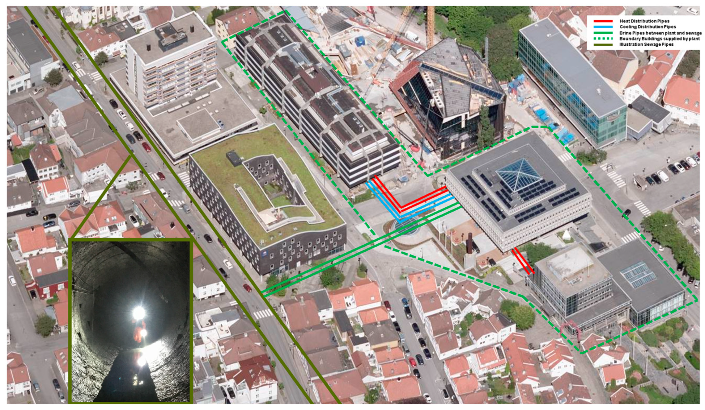
2.1. Case Study Description

The case study plant and the Municipality of Stavanger’s contribution to Triangulum project, detailed in a previous work [33], are highly ambitious EU-funded thermal energy initiatives. Operational since 2017, the plant utilizes wastewater heat pumps and biogas boilers to produce 1.5–2.5 GWh of thermal energy annually, serving three municipal buildings with heating and cooling.
Wastewater was chosen as the most feasible thermal reservoir for the project after a thorough evaluation that balanced investment and operational costs, CO2 emission reduction, and practical implementation. In the densely built urban areas, alternatives such as geothermal boreholes and seawater were deemed unsuitable due to challenging local conditions. Located approximately 100 m directly from the energy plant, a main municipal storm and sewage water tunnel run through rock beneath Stavanger, Norway. This nearly circular tunnel, about 4 km long and 3.3 m in diameter, was drilled through the bedrock in the 1980s. The tunnel starts at an elevation of 2.4 m above sea level and ends at 1.6 m, with the section near the plant being about 2.0 m high, located 7 m below the plant’s floor.
The wastewater plate heat exchanger system was identified through an internet-based, non-academic search and subsequently developed in collaboration with a potential technology supplier. Key design parameters of this system include the wastewater flow rate and temperature, the geometry of the tunnel, and the specifications of the heat pump and brine system, such as flow rate and design temperature levels.
To determine the design flow rate, historical measurements of the wastewater flow rate were correlated with rainfall data, as illustrated in Figure 2. The figure represents daily values averaged over 24 h for flow, rainfall, and the resulting water height in the tunnel, based on data from 2015. From these historical data, the baseline wastewater flow rate for the heat exchanger design was set to 250 L per second. However, the data indicated that this flow rate can increase significantly following rainfall events. Historical wastewater temperatures had been observed to vary between +7 °C and +16 °C, and the design temperature levels for the brine system were set to +1 °C at the inlet and +5 °C at the outlet of the heat exchangers in heating mode. To calculate the brine flow rate required to achieve the 360 kW design heat extraction, the following formula was used [36]:
Q ˙ = m ˙ × c p × ( T o u t T i n ) ,
where Q ˙ (in kW) represents the net rate of heat transfer from the wastewater to the heat pump brine, or vice versa, m ˙ (in kg/s) is the mass flow rate of the heat pump brine, c p (in kJ/kg·K), is the specific heat capacity of the heat pump brine, here specified for MEG20 (a 20% solution of Monoethylene Glycol), and T i n and T o u t (in K), are the temperatures of the heat pump brine entering and exiting the heat exchangers, respectively.
Through a public procurement process, several European suppliers were invited to submit their proposals and project costs based on the specified design parameters. Given that the tunnel is sealed during wastewater operations and the installation point is far from the nearest entry (see Section 4 for details), the municipality requested a maintenance-free system. A team consisting of Dansk Kloak RenoveringsTeknik [37] and UHIRG [17] was selected to install UHRIG’s custom-built stainless steel heat exchanger system, named Therm-Liner, directly on the tunnel wall. The Therm-Liner system, characterized by its lack of moving parts and absence of electrical components, minimizes maintenance needs.
The final configuration of the heat exchanger system, as shown in Figure 3, included 108 heat exchanger plates, each weighing 100 kg and measuring 1.0 m in length, shaped according to the design sketch. To ensure equal distribution of the brine fluid across all heat exchangers, the return pipe was reversed.
Three tunnels were drilled through the mountain to connect the energy plant with the wastewater tunnel: two are used for the supply and return of energy brine pipes, and one houses utilities such as fiber cables and a temperature sensor for monitoring wastewater temperature.
Figure 4 presents an aerial view diagram of the energy plant building and its connections to the wastewater tunnel. The red and blue lines show the heating and cooling distribution pipes from the plant to neighboring buildings, while the brown line approximates the location of the wastewater tunnel. The solid green line indicates the tunnels and pipes from the plant to the wastewater, and the dashed green line denotes the buildings included in the project. In Section 4, further elaboration on challenges during the planning and installation phases is given.
The main design targets for the project related to wastewater heat pumps are presented in Table 1 [33]:

2.2. Methodology for Evaluating the Performance of the Heat Pumps and Wastewater Heat Exchangers

The primary goal of this evaluation was to investigate the long-term performance of the heat pumps and wastewater heat exchangers while identifying any short-term issues that suggest opportunities for improvement.
Historical operational data were collected and processed to calculate the key performance parameters. Tables summarizing several years of operational data were compared against the design of the targets. Duration curves were developed to detail the thermal energy production, including contributions from wastewater heat, electricity used for compressors, gas for boilers, and recovered heat from cooling production. Section 4 presents a statistical analysis of key parameters, along with a series of scatter plots from the two heat pumps, to visualize relationships and performance trends.
While cooling production and seasonal cooling parameters were calculated in this study, the detailed analysis of heat pump operation excludes the cooling mode. This exclusion is due to the relatively minor contribution of cooling to the overall thermal energy production and the challenges presented by rapid ON-OFF operation cycles. For further discussion on the cooling production, readers are referred to previous work [33].

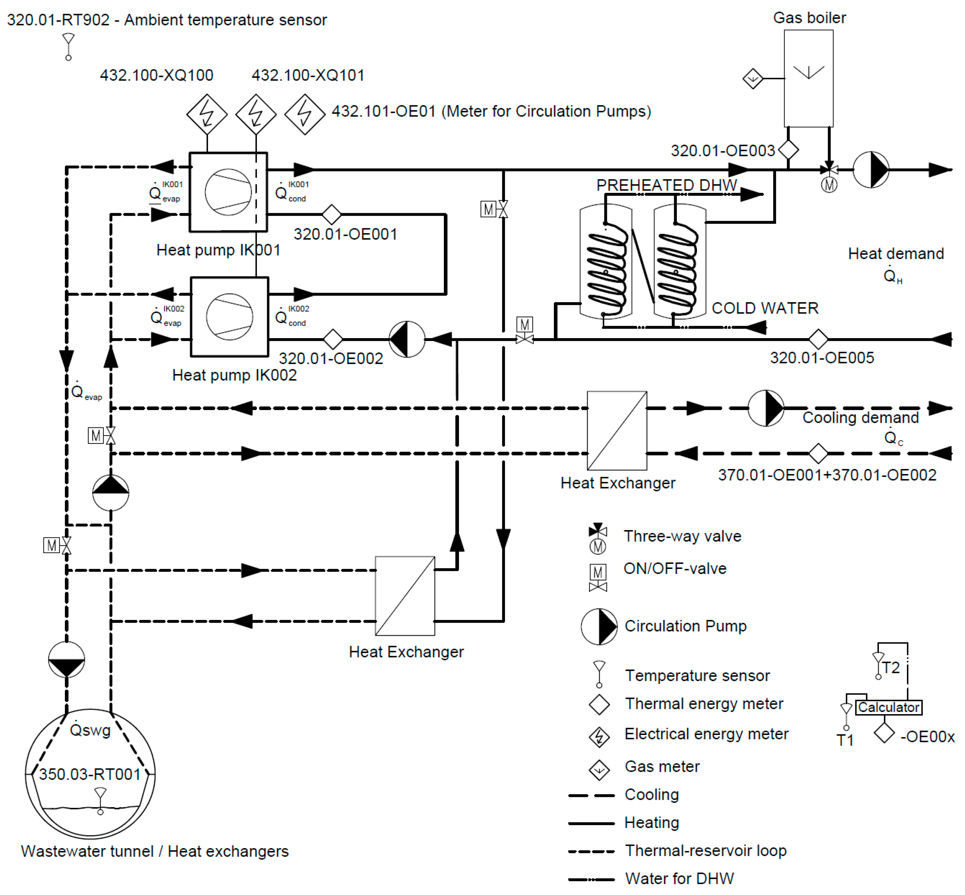
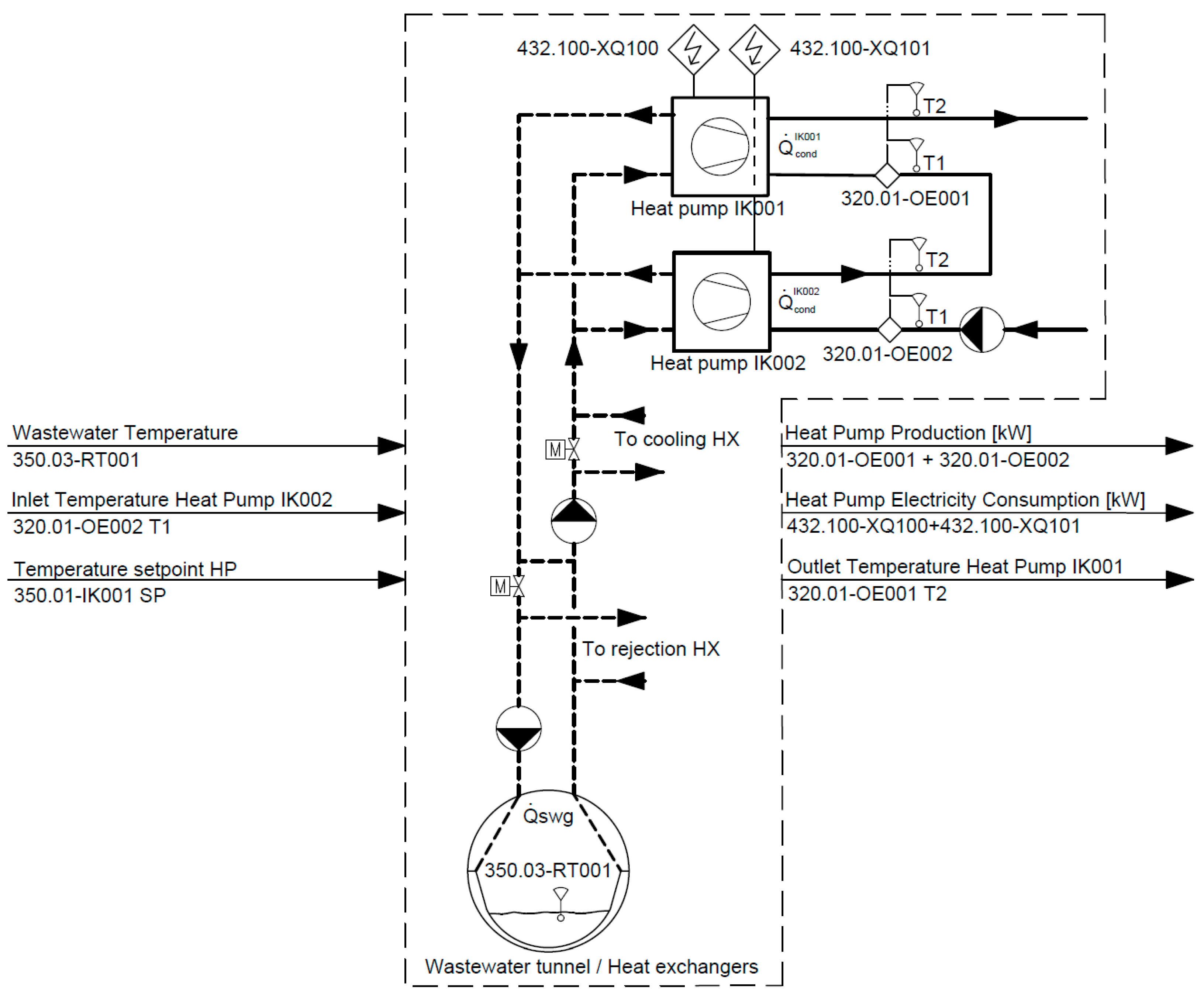
2.2.1. System Design and Relevant Sensors

Figure 5 illustrates a schematic of the integrated system. The system consists of two heat pumps, tagged as IK001 and IK002, connected in series on the condenser side and in parallel on the evaporator side. Both heat pumps have a nominal heat capacity of 250 kW, with four semi-hermetic reciprocating compressors, two of which are equipped with capacity control to manage load demands effectively. The design capacity allows for a high base load heat contribution and meets the maximum cooling demand. The machines have two operational modes to adapt to varying thermal demands.
In heating mode, the operation is controlled by outlet temperature setpoints on the condenser water side, with the first heat pump in the series set to operate at a temperature that is 5K lower than the second one. The heat pumps are connected to two accumulator tanks on the condenser side, serving as a zero-pressure junction between the heat pumps and the heat distribution loop. A gas boiler acts as the peak load and backup heating unit. Low-temperature heat is primarily extracted from the wastewater, while also utilizing any excess heat from simultaneous cooling production.
Cooling mode is defined based on a general assumption, that there is no demand for heating in this mode. The heat pumps are managed by outlet temperature setpoints at each evaporator, normally set equal to 10 °C. Excess heat from the cooling production is rejected to the wastewater via the condenser and a rejection heat exchanger. Despite the assumption of no heating demand, the gas boiler can be activated to provide heating. In both modes, the flow rates across each condenser and evaporator are close to constant.
All sensors utilized to monitor system performance are presented in Figure 5. Thermal energy meters are installed at each condenser, at the gas boiler, and within the heat and cooling distribution systems. Each thermal energy meter is equipped with a flow meter and two calibrated temperature sensors. Additionally, three meters are installed for measurement of electricity consumption: one at each heat pump condenser and one for other electrical equipment, primarily circulation pumps.

2.2.2. Data Capture

Data for this analysis were obtained from the thermal energy plant’s control system, Citech Scada [38], covering the period from September 2020 to May 2024. These data were manually captured at varying points in time, with a resolution varying from 5 to 60 min. To ensure analytical consistency, data recorded at five-minute intervals were aggregated into 60 min mean values. For the performance evaluation, only data from two full years, 2022 and 2023, were available and used.

2.2.3. Performance Parameters

In this section, key evaluation parameters based on the energy meters shown in Figure 5 are defined. These parameters establish the baseline for all evaluations conducted in this work. In the analysis, both instantaneous values and accumulated data were examined. Instantaneous values were represented by hourly averages.
The Coefficient of Performance (COP) is a primary performance measure for the heat pump, indicating its performance by comparing the ratio of heating or cooling output to electrical energy consumed [39]. The heat pump can operate in either heating or cooling mode, each affecting the COP calculation. For heating and cooling, the COP is determined as follows:
COP heat = Q ˙ c o n d W ˙ h p
COP cool = Q ˙ e v a p W ˙ h p = EER
where Q ˙ e v a p is the heat extracted at the evaporator, Q ˙ c o n d is the heat output at the condenser and W ˙ h p is the electrical input to the heat pump, all measured in kWh/h. The cooling COP is also known as the Energy Efficiency Ratio (EER). When the system operates in heating mode, it may produce both heating and cooling simultaneously, utilizing low-temperature excess heat from cooling as a heat source. If the cooling demand is lower than the heat extracted at the evaporator, the total COP of the heat pump system is defined as follows:
COP tot = Q ˙ c o n d + Q ˙ c o o l   W h p ˙ ,
where Q ˙ c o o l is the actual cooling demand, measured within the cooling distribution system. In cooling mode, all excess heat produced at the condenser is rejected to the wastewater. Since there is no thermal energy meter on the evaporator side of the system, the analysis relies on the following well-known simplification to estimate the cooling production at the evaporators:
Q ˙ e v a p = Q ˙ c o n d W ˙ h p ,
This formula is based on the premise that the heat removed at the evaporator can be calculated by subtracting the work done by the heat pump from the heat rejected at the condenser. This is a common practice in thermodynamic calculations where direct measurements are not available [39].
The following energy meters are utilized to describe the system’s heating and cooling production:
  • Heat production is measured by the heat distribution loop energy meter, Q ˙ h e a t   320.01-OE005 .
  • Cooling production is measured by the sum of the cooling distribution loop energy meters, Q ˙ c o o l = 370.01-OE001 + 370.01-OE002 .
To calculate the COP and EER for the heat pumps, the following configurations of energy meters are utilized:
COP heat IK001 = 320.01-OE001 432.100-XQ100 ,   EER cool IK001 = 320.01-OE001-432.100-XQ100 432.100-XQ100 ,
COP heat IK002 = 320.01-OE002 432.100-XQ101 , EER cool IK002 = 320.01-OE002-432.100-XQ101 432.100-XQ101 ,
COP heat heat   pumps = 320.01-OE001 + 320.01-OE002 432.100-XQ100 + 432.100-XQ101 ,
E E R c o o l i n g h e a t   p u m p s = 370.01-OE001 + 370.01-OE002 432.100-XQ100 + 432.100-XQ101 ,
COP total heat   mode = 320.01-OE001 + 320.01-OE002 + 370.01-OE001 + 370.01-OE002 432.100-XQ100 + 432.100-XQ101 ,
The heat extracted at the evaporators is estimated using Equation (5) and the following energy meter combinations:
Q e v a p I K 001 ˙ = 320.01-OE001-432.100-XQ100
Q e v a p I K 002 ˙ = 320.01-OE002-432.100-XQ101
Q ˙ e v a p = Q e v a p I K 001 ˙ + Q e v a p I K 002 ˙
In heat mode, the heat pumps operate to meet the temperature setpoints at the condensers. However, there may still be a demand for cooling, in which case any excess heat is diverted to the evaporator. This process is known as free cooling. Free cooling is prioritized over extracting heat from the wastewater; therefore, the wastewater heat extraction process is calculated as follows:
Q ˙ w w = Q ˙ e v a p Q ˙ c o o l ,
and using the energy meters, the wastewater heat extraction is determined from:
Q ˙ w w = ( 320.01-OE001 + 320.01-OE002 ) ( 432.100-XQ100 + 432.100-XQ101 ) ( 370.01-OE001 + 370.01-OE002 )
In cooling mode, heat is rejected to the wastewater and calculated as follows:
Q ˙ w w = 320.01-OE001 + 320.01-OE002
For assessing seasonal performance, the definitions of performance metrics align with those used for momentary evaluations but rely on accumulated data collected over a defined seasonal period instead of instantaneous values. The Seasonal Coefficient of Performance (SCOP) measures the performance of a heat pump over one year or a specific heating or cooling season. It takes into account variations in the COP under different operating conditions encountered throughout the year [40]. Here, each ‘season’ is defined as a year, consisting of 8760 h. For example, Seasonal Coefficient of Performance for heating for the heat pump (SCOPheat) is defined as follows:
SCOP heat = Q c o n d W h p ,
where Q c o n d is the total heat produced at the heat pump condenser over a season, and W h p is the total electricity input to the heat pump during the same season. The total plant performance of a year, the Seasonal Performance Factor (SPF), is defined as follows:
SPF total = Q h e a t + Q c o o l W h p + W g a s + W p u m p s  
where Q h e a t represent the total heat production, Q c o o l is the total cooling production, W g a s   accounts for gas consumption and W p u m p s represents the electricity consumption for circulation pumps. Using the energy meters, the SPFtotal can be calculated from actual readings as follows:
SPF total = 320.01-OE001 + 320.01-OE002 + 320.01-OE003 + 370.01-OE001 + 370.01-OE002 432.100-XQ100 + 432.100-XQ101 + 320.01-OE003 + 432.101-OE01
Note that the heat pump system is connected to two thermal accumulators equipped with internal heat exchanger coils for pre-heating Domestic Hot Water (DHW). In the calculation of COP and the SPF above, the heat pump’s contribution to DHW is factored in.
To evaluate the efficiency of the heat pump process itself, the System Efficiency Index (SEI) [40], sometimes known as the Carnot efficiency, is used. The SEI is calculated as the ratio of the actual COP to the COP of an ideal, reversible Carnot process (COPC). This ideal COP serves as a theoretical benchmark, rooted in the laws of thermodynamics, for a process that transfers heat energy to a higher temperature level. For heating (h) and cooling (c), the Carnot COP can be expressed as follows:
COP heat , C = T h , r e f T h , r e f T c , r e f ,  
COP cooling , C = T c , r e f T h , r e f T c , r e f ,  
where T h , r e f and T c , r e f are reference temperatures for the two reservoirs that the heat pump operates between, represented by the average between the inlet and outlet temperatures on the condenser and evaporator, respectively. The temperature difference, T h , r e f T c , r e f , is defined as the heat pump temperature lift for future evaluations. The design or measured COP is then divided by the ideal COP, and this ratio, less sensitive to changes in temperatures and flow rates than the COP alone, equals the SEI. The SEI calculations for systems supplying heat are as follows:
SEI heat = COP heat COP heat , C ,  
According to the report Method and Guidelines to Establish System Efficiency Index during Field Measurements on Air Conditioning and Heat Pump Systems [40], SEI values for heat are categorized as follows for assessing performance quality:
  • 0–0.2: Unacceptable
  • 0.2–0.35: Poor
  • 0.35–0.45: Good
  • >0.45: Excellent
To evaluate the operational efficiency of heat pumps under varying load conditions, a straightforward metric known as the Electrical Load Factor (ELF) is defined by the following formula:
ELF   ( % ) = ( A c t u a l   E l e c t r i c t y   C o n s u m p t i o n   o f   H e a t   P u m p M a x i m u m   E l e c r i c t i y   C o n s u m p t i o n   o f   H e a t   P u m p   ) × 100

2.2.4. Limitations

The key limitations identified in the analysis are as follows:
  • Gas boiler contribution: The energy contribution from the gas boiler used in the performance calculations is measured by the thermal energy meter 320.01-OE003, which is positioned between the gas boiler and the heat distribution system. However, actual gas consumption data from the gas company was unavailable due to data capture errors. Previous studies have indicated that the boiler’s efficiency is below expectations, but this error is not attributed to the heat pump system design, but rather to the control strategy implemented in this specific part of the system. Consequently, the SPF values reported here may be higher than the real values, as more gas was used than measured at 320.01-OE003.
  • Reduced demand due to refurbishment: The plant was originally designed to supply three buildings with thermal energy. During the data collection period, one of these buildings had been temporarily removed from the system for refurbishment. Thus, during the whole measurement period, the heat pumps have had an overcapacity relative to the maximum demand. Consequently, the utilization rate of the heat pump may appear disproportionately high when compared to typical systems designed to balance both base and peak load units. Additionally, the design production numbers presented in Table 1 are expected to be higher than those measured.

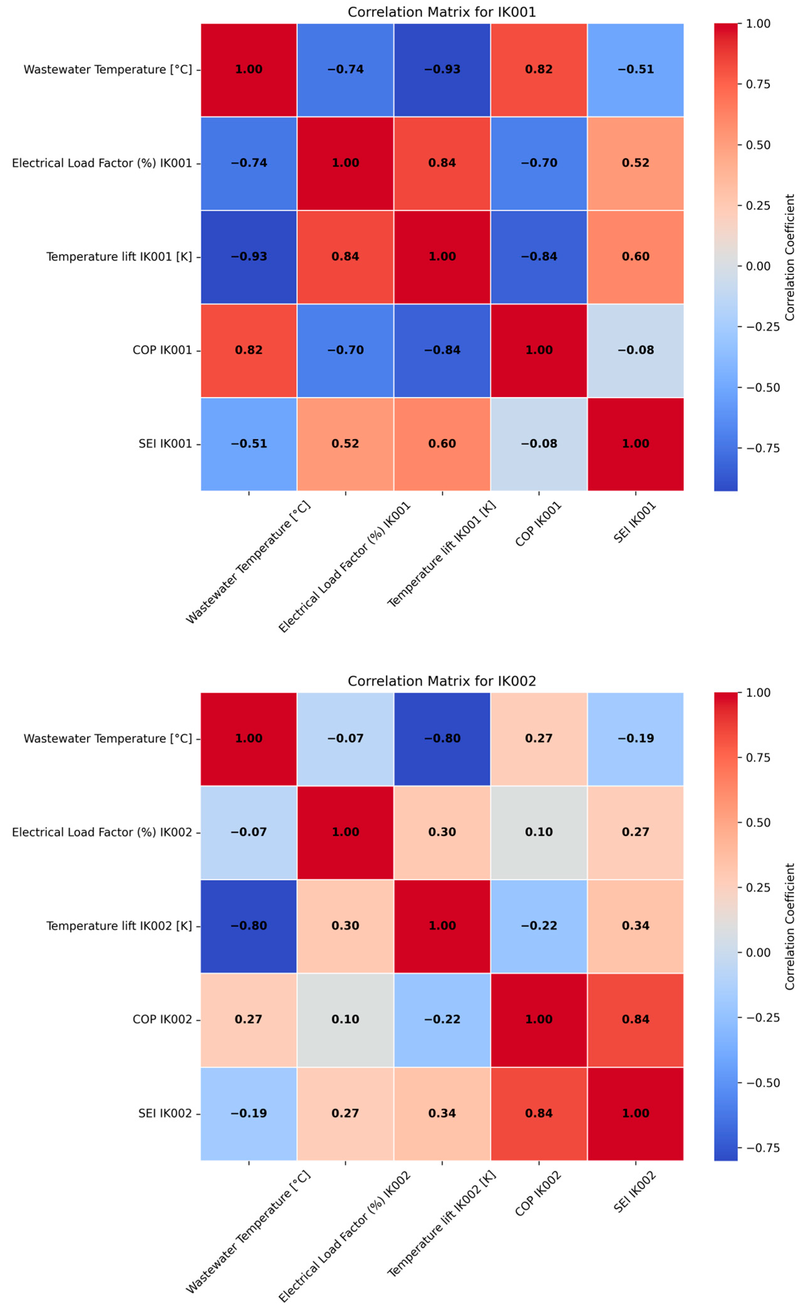
2.3. Statistical Evaluation Using Correlation Analysis

Correlation analysis was used to evaluate how the operational parameters affect the heat pump. Pearson’s coefficient, r, was utilized to measure and quantify the strength and direction of linear relationships between variables [41]:
r = ( x i x ¯ ) ( y i y ¯ ) ( x i x ¯ ) 2 ( y i y ¯ ) 2 ,    
where:
  • x i and y i are the individual sample points indexed i,
  • x ¯ and y ¯ are the means of the x and y data sets.
  • The result, r, ranges from −1 to +1, where:
  • An r-value of +1 indicates a perfect positive linear relationship,
  • An r-value of −1 indicates a perfect negative linear relationship,
  • An r-value of 0 indicates no linear relationship between the variables.
All statistical analyses were performed using Python, utilizing libraries such as Pandas for data manipulation, NumPy for numerical operations, and Statsmodels for performing statistical tests and regression analyses [41].

2.4. Artificial Neural Networks for Evaluating the Heat Pump Performance

To evaluate the performance of heat exchangers over time, Artificial Neural Networks (ANNs), an ML method with substantial popularity in various fields such as mathematics and engineering [42], were utilized. ANNs are favored for their ability to model complex relationships and predict outcomes from large datasets. The methodology adopted for this study is detailed in previous work [43]. Readers seeking a deeper understanding of the specific technique are encouraged to consult the relevant literature in the field of ML [41].

2.4.1. Model Structure and Development

The ANN model was designed to predict heat pump performance based on inlet conditions and setpoint temperatures. As shown in Figure 6, the model considers the two heat pumps as a single production unit with one inlet and one outlet on the condenser side. Model inputs include the water temperature entering the first condenser and the production setpoint of the second heat pump, while the wastewater temperature serves as the input for the evaporator side. The model outputs are total heat production, electricity consumption, and the system’s outlet temperature.

2.4.2. Training, Validation, and Test Data with Emphasis on Fouling Assessment

Data from September 2020 to June 2024 were utilized to develop the ANN, organized into distinct sets to specifically determine the impact of fouling on system performance:
  • Training Set: Data from 2020 to 2022 represented the training set, with 20% reserved for validation during the training phase to fine-tune the model.
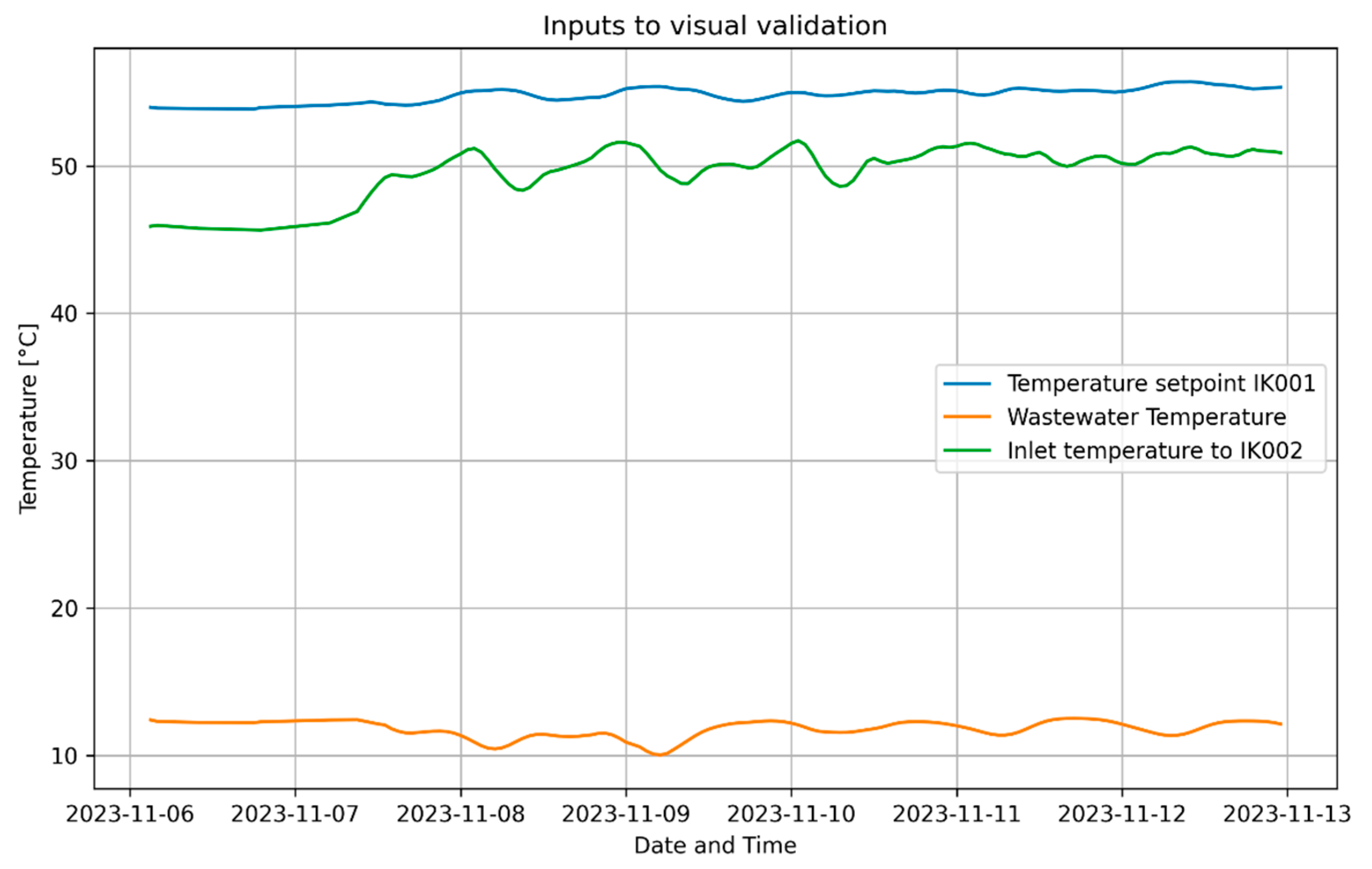
  • Data from 2023 were used for “visual validation,” evaluating the model configuration, testing various input/output parameters, and adjusting hyperparameters. This stage was important for identifying potential faulty operations and providing a practical check against real-world conditions.
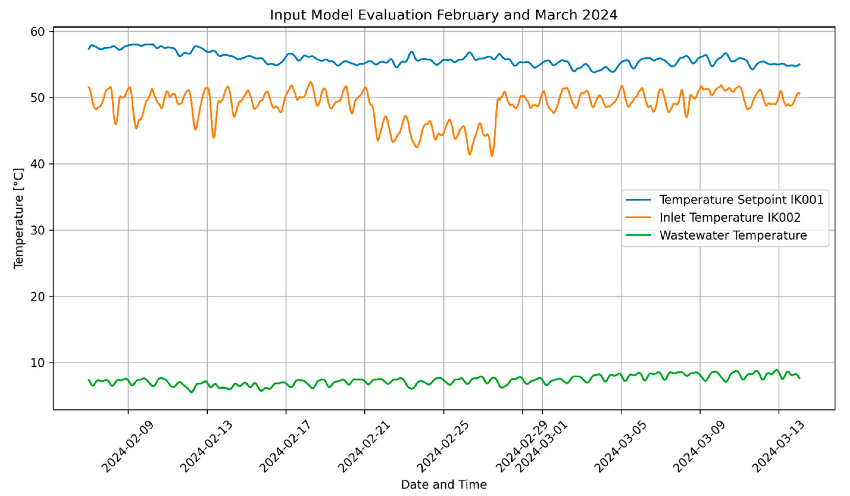
  • Test Set: Data from 2024, referred to as “unseen” data, were used for final testing to confirm the model’s effectiveness. The test aimed to verify that the model, trained on data from earlier years, could accurately predict system performance under current conditions. A successful outcome would indicate that the system’s performance has remained consistent over the years, free from significant deviations due to fouling or other inefficiencies. Positive results could also suggest the model’s potential for ongoing monitoring and diagnostic applications.

2.4.3. Data Preparation

To ensure the quality and relevance of the training data, thorough data processing was performed before developing the ANN. Initially, all rows with missing values were removed to guarantee consistency in the dataset. Then, outlier detection was performed using a Z-score approach, which measures how far each data point deviates from the mean in terms of standard deviations [44]. Data points with a Z-score above 3 were considered outliers and excluded. This removed 3223 rows of the dataset, initially consisting of 25,242 rows.
The dataset was further processed using a Savitzky-Golay filter, a method that involves using a moving window to fit a polynomial among the points within that window [45]. A second-order polynomial was selected to smooth segments of eleven consecutive data points, effectively capturing fluctuations throughout the day. This approach preserves critical features such as peaks and minima through its polynomial fitting technique. A visual representation of the filtering for heat production, electricity consumption, and wastewater temperature is provided in Figure 7.
Next, a more hands-on evaluation was conducted to ensure the dataset reflected healthy operational conditions. Initially, rows where the COP exceeded a threshold of 5.0 were removed to filter out instances where a small amount of heat was recorded after the heat pump had shut down, eliminating a total of 170 rows for the heat pump combined.
Then, erroneous operations of the heat pumps, initially identified through manual examination of time series data and using the visual validation data actively, were excluded. Note that this was a coarse manual procedure, and there may be erroneous instances within the final data set. Specifically, instances where the temperature difference between the outlet temperature and the setpoint was high while the power output was lower than a threshold were filtered out. These situations indicated that one or several of the compressors were out of order. Additionally, there were cases where heat pump IK002 was significantly more active than IK001, which, due to active setpoint configurations, suggested operational errors with IK001. These filtration steps led to the removal of 8515 rows.
The final filtration step involved excluding data from the peak summer months, June, July, and August, to focus on the heating season. Through the filtration steps, the dataset was reduced to 10,481 entries from an initial count of 25,242. Notably, the removal of 8515 rows due to erroneous operations is particularly significant as it represents almost a full year’s worth of data where one or both heat pumps had faulty operation. This not only underscores the importance of the data cleaning process but also highlights the critical need for consistent monitoring and maintenance of these systems, given the frequency of operational errors. This study was performed without access to maintenance logs. Had these logs been available, they could have enabled more precise identification of operational errors, thereby making the data cleaning more systematic than the current approach.

2.4.4. Model Construction and Training

After cleaning, the training dataset was separated into the features and labels as defined in Figure 6. Both features and labels were scaled using a StandardScaler [41] to normalize the data, ensuring no feature dominated the model due to its scale. The model was structured using a sequential layout consisting of an input layer, three hidden layers, and an output layer. Each layer employed a Rectified Linear Unit (ReLU) activation function, except for the output layer, which used linear activation [41].
Training was conducted using the Adam optimizer and the Mean Squared Error loss function. The model underwent training for 5000 epochs, with early stopping implemented to prevent overfitting. Early stopping monitored the validation loss and halted training if no improvement was seen for 50 consecutive epochs. Model checkpoints were utilized to save the best-performing model based on validation loss [41].
The selected approach ensured a robust and thoroughly trained ANN, with specific steps taken to prevent overfitting. Table 2 summarizes the hyperparameters and training settings used in the model’s development.

2.4.5. Performance Metrics

The performance of the ANN was assessed using the 2024 test set, which was separated from the training data to provide an unbiased evaluation of the model’s predictive accuracy. The same performance metrics were used during the visual validation phase. Mean Absolute Error (MAE) quantifies the average magnitude of errors in the model’s predictions [41]. It is calculated as follows:
M A E = 1 n i = 1 n | y i y i ^ | ,
where n represents the number of data points and y i and y i ^ are actual and predicted values of parameters. MAE provides a straightforward measure of error magnitude without considering direction.
Root Mean Square Error (RSME) measures the overall magnitude of errors, emphasizing larger deviations due to the squaring of each error [41]. RMSE is particularly sensitive to outliers and provides a more conservative estimate of model performance:
R S M E = 1 n i = 1 n ( y i y i ^ ) 2
Mean Absolute Percentage Error (MAPE) estimates the average percentage error between the model’s predictions and observed data, giving a sense of error in relative terms [46]. MAPE is especially useful when comparing the performance of models across different scales or units. However, it should be used with caution when the actual values are close to zero, as it can lead to disproportionately high errors and may distort the overall performance assessment:
M A P E = 1 n i = 1 n | y i y i ^ y i | ,
Together, these metrics offer a comprehensive view of model accuracy, with MAE providing a baseline average error, RMSE highlighting larger errors, and MAPE offering a percentage-based evaluation. Additionally, the Maximum Absolute Error is reported, which captures the single largest error across all predictions, helping to identify the worst-case scenarios in model performance.

2.5. Manuscript Preparation and Editorial Assistance

In addition to the technical methodologies, during the development of this manuscript, the OpenAI GPT-4 model was employed for editorial assistance. Specifically, GPT-4 aided in refining sentence structures and providing word choices, enhancing the clarity and readability of the text. It also played a role in explaining and summarizing complex sections from the referenced literature.

3. Results

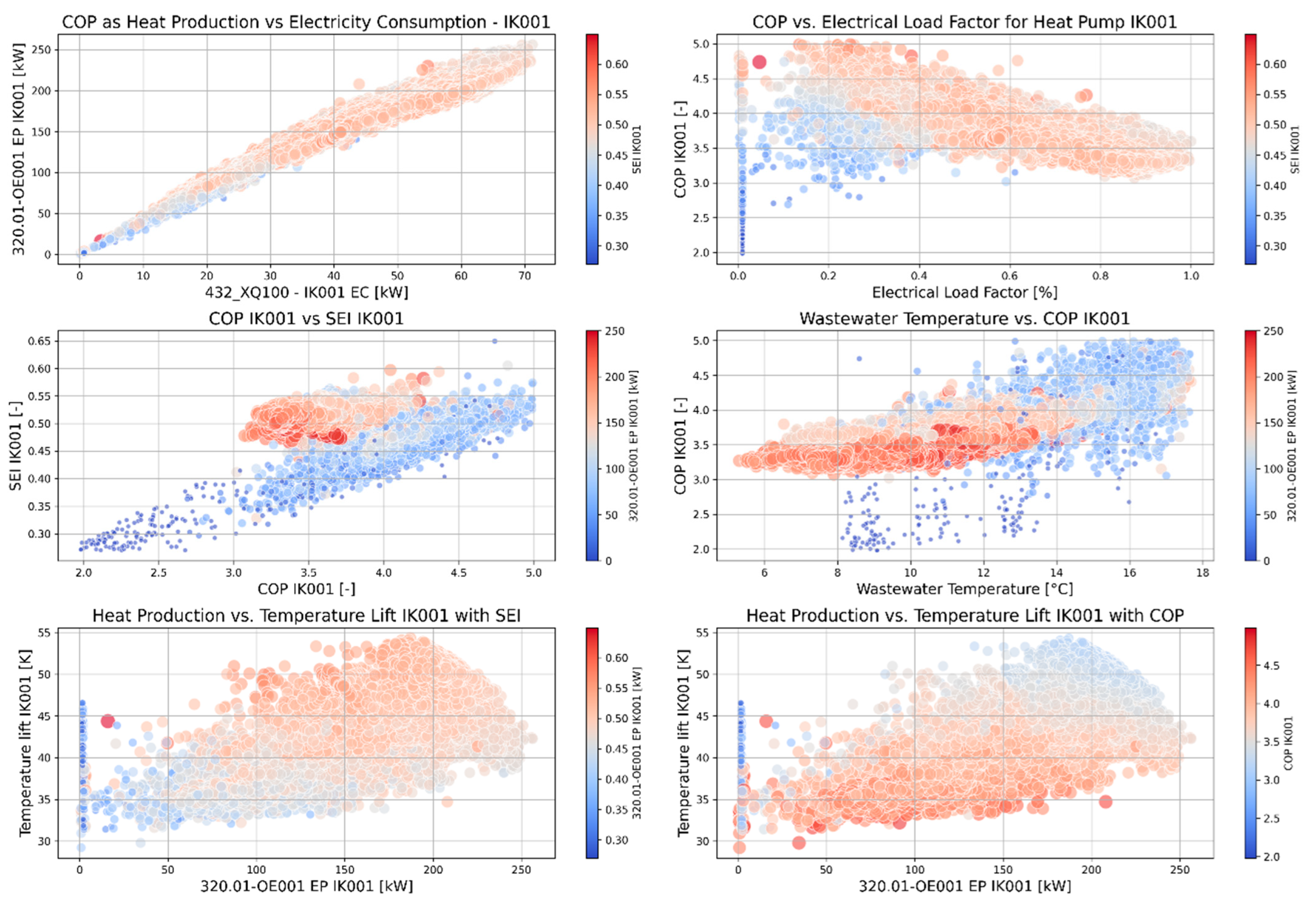
3.1. Evaluation of Heat Pump Performance

The annual energy results for the plant are presented in Table 3 for the years 2022 and 2023. Additionally, duration curves for the gas boiler and the components contributing to heat pump production for the same years are displayed in Figure 8 and Figure 9. These duration curves are based on sorted values of heat production from maximum to minimum, with corresponding data for gas and electricity consumption, wastewater heat, and excess heat from cooling, all linked to their contributions to the maximum production levels.
From the accumulated energy results, the following can be observed:
  • The system for heating and cooling production, excluding peak heating for DHW, has produced its energy with an SFP between 2.7 and 2.8, which is considered highly satisfactory.
  • The heat pumps have met most of the thermal demand for the two operational buildings, with the gas boiler contributing minimally. This outcome aligns with expectations and contrasts with the period of 2019 to 2020, when three buildings were operational [33] and both the heat pump and gas boiler had significantly higher contributions. It is important to note that data from 2019 to 2020 are not as detailed as those presented in this study.
  • There have been no significant peaks in gas boiler usage, and the boiler has primarily served as a backup unit during these years.
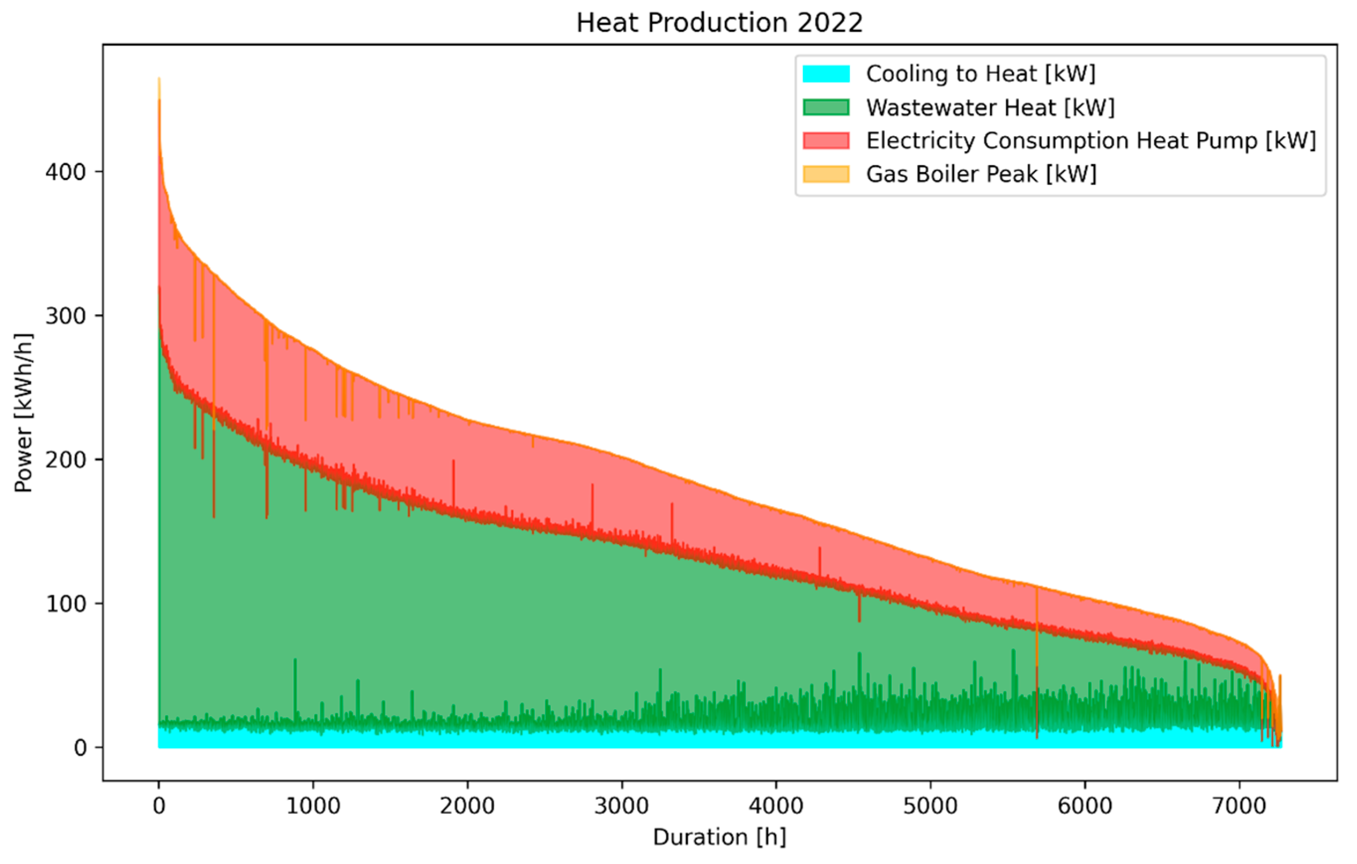
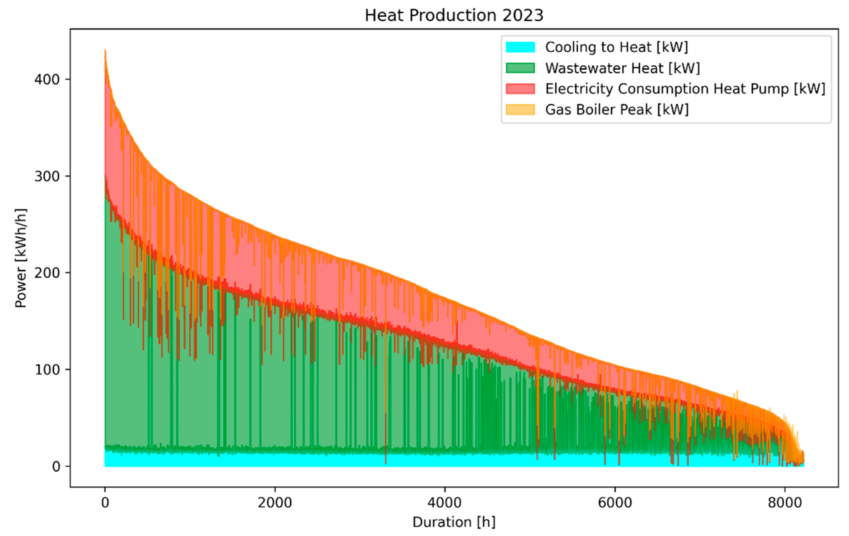
  • Wastewater heat has been the predominant low-temperature heat source, contributing to more than 60% of the total heat produced in both evaluated years, indicating that the heat exchangers are performing in line with expectations.
  • While the power contribution of excess heat from cooling is small, averaging about 14 kW, it has been consistent throughout the years. Though not as important in a system where the heat extraction does not significantly influence the source temperature, a steady contribution of 14 kW, equivalent to 120,000 kWh/yr, could significantly benefit a geothermal heat pump system.
  • The production from the two heat pumps has been highly uneven; IK001 has produced 87% and 75% of the heat in the respective years, while IK002 has produced 13% and 25%. The SCOP values for IK001 and IK002 were 3.6/3.6 and 3.4/3.5, respectively, perfectly in line with design expectations. Given that IK001, as the second pump in the series, has been set to produce a temperature 5K above that of IK002 and still achieved a higher SCOP, this suggests that the operational strategy and set-point scheme for IK002 should be re-evaluated.

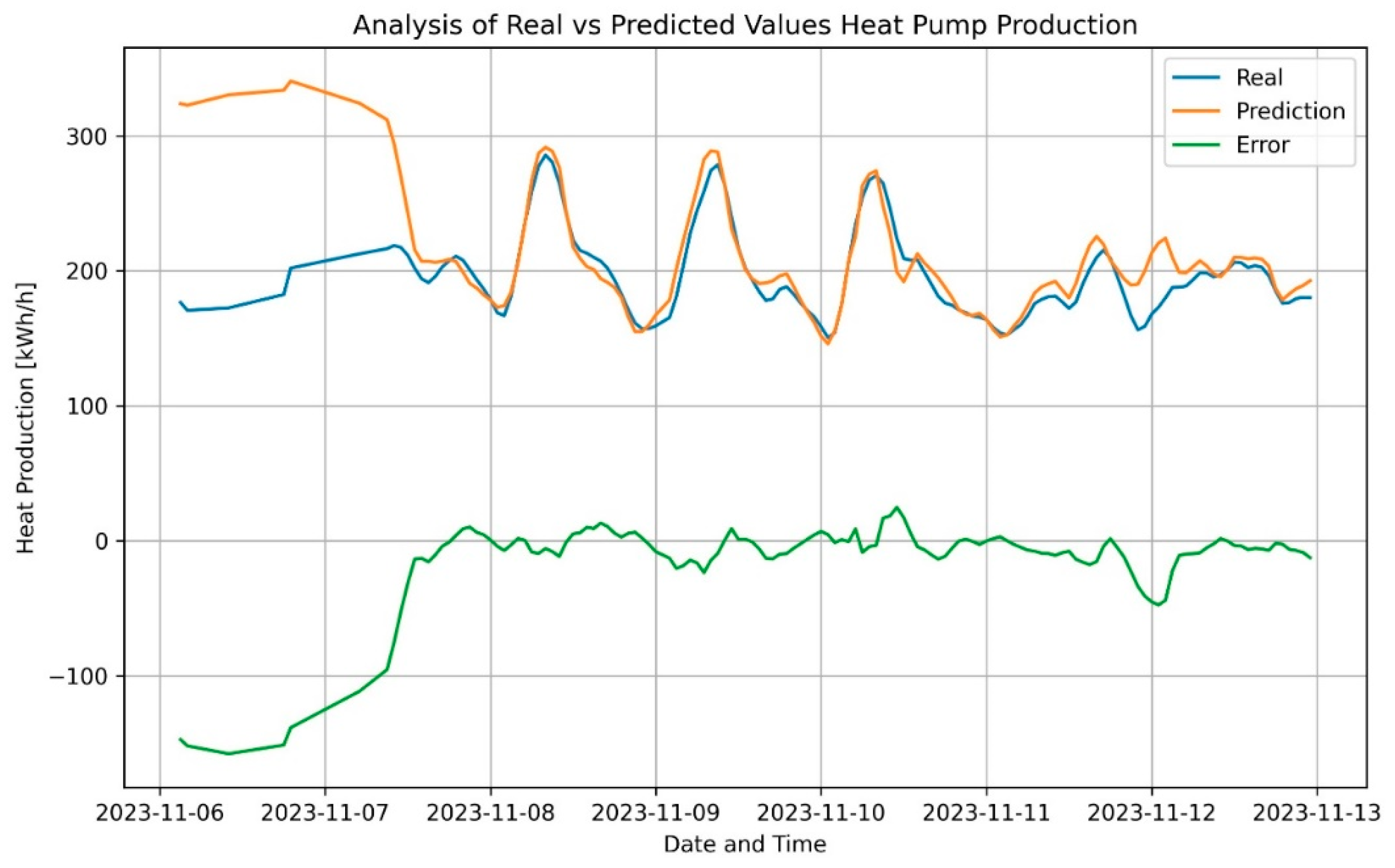
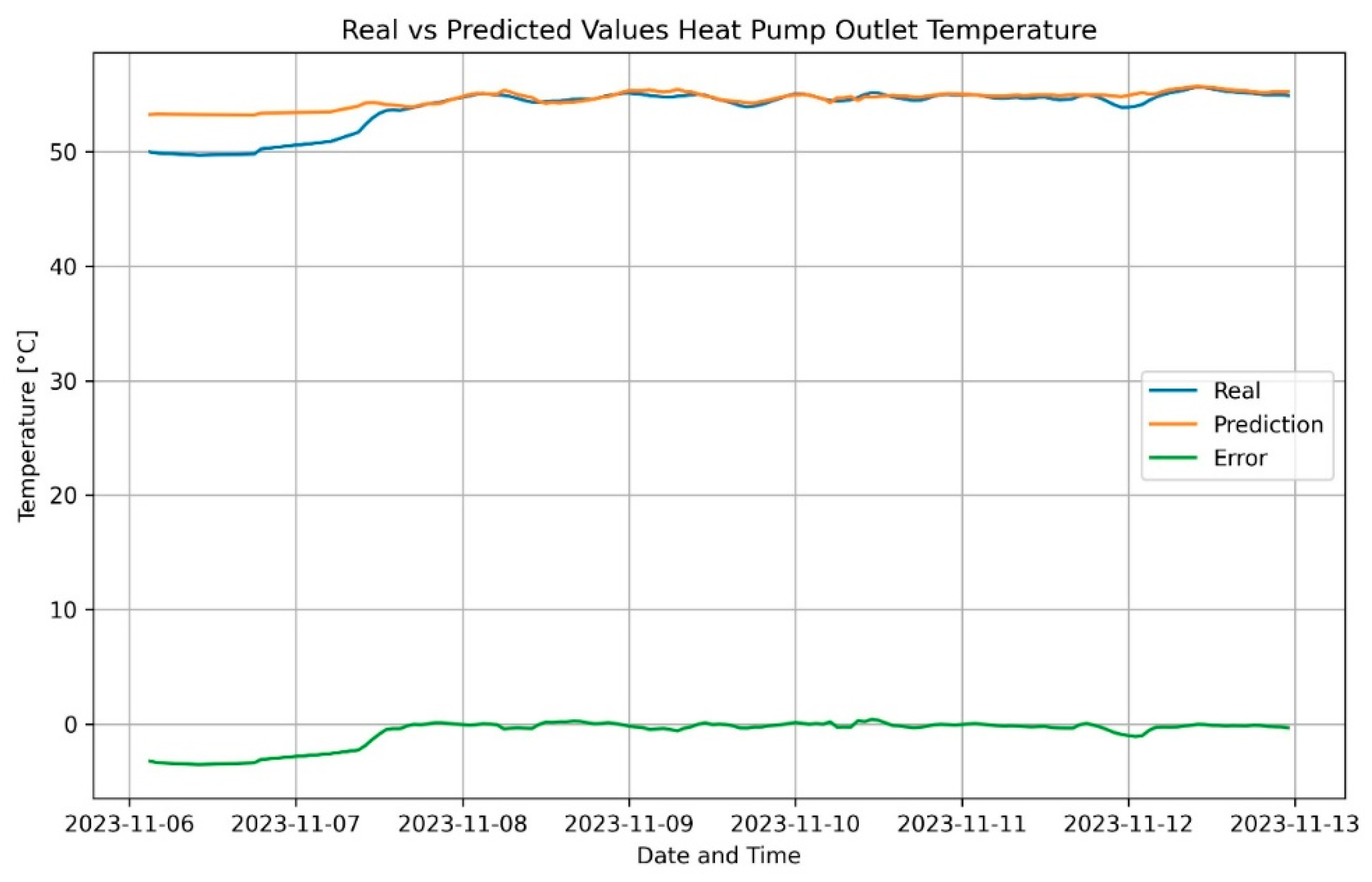
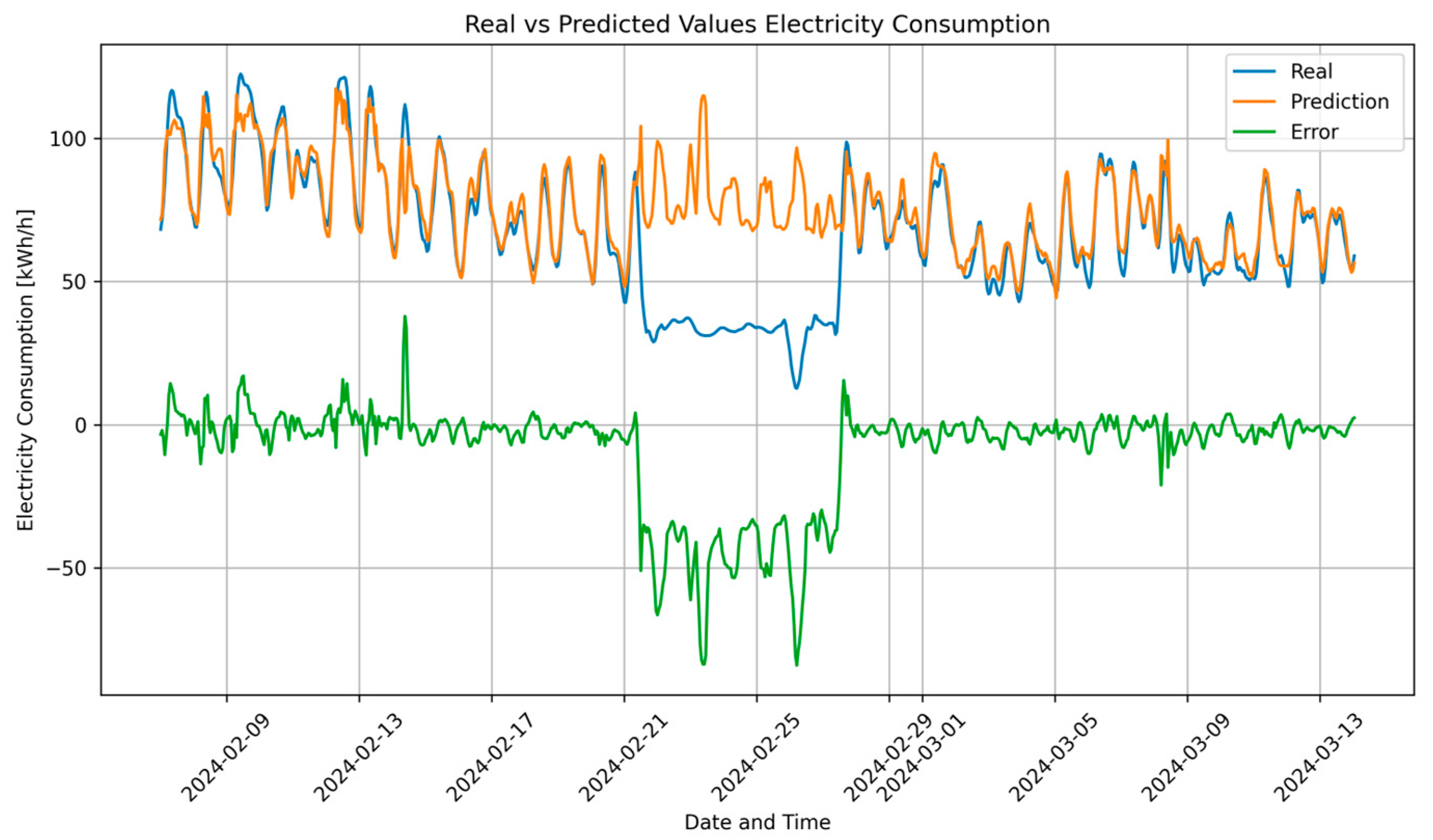
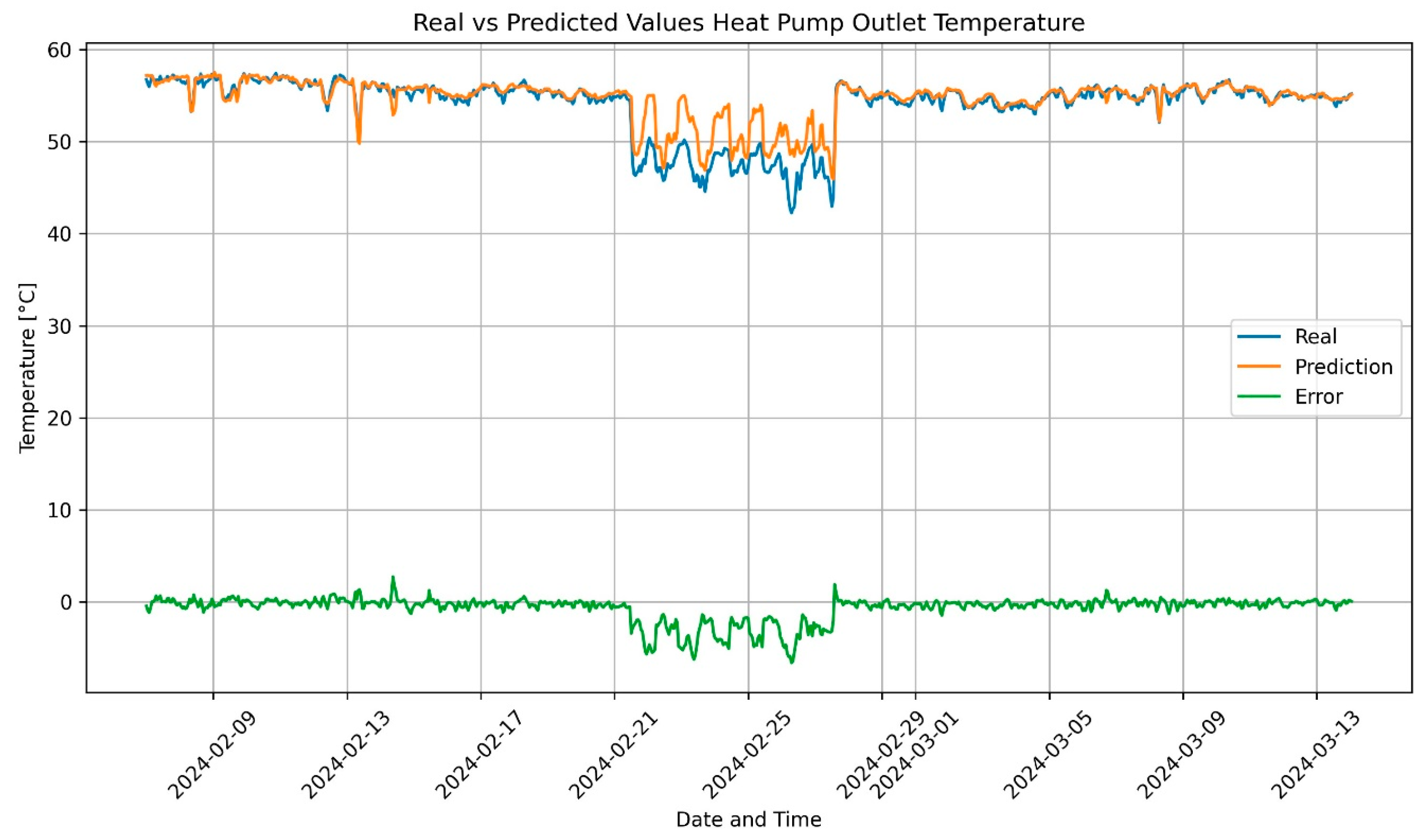
3.2. Prediction of Heat Production, Electricity Consumption, and Outlet Temperature Using ANN

The results of the ANN model are detailed in the figures and tables that follow. The model was initially trained on data from 2020 to 2022. During the training process, the model results were continuously visually evaluated using data from 2023, which served as an aid through data processing, alongside standard validation principles. Finally, data from a month in 2024 were used to test the final model configuration.
Figure 10 illustrates an example of the input data used for the visual validation of the final model configuration. Figure 11 and Figure 12 display the model’s predictions alongside the actual values for heat production and outlet temperature in the same period, respectively. These figures also include the error, calculated as actual minus predicted values. The results of the electricity consumption follow a similar pattern as the heat production.
During visual validation, the model exhibited significantly higher errors during specific periods. These included the initial days and a brief period on 12 November, as highlighted in the figures. Notably, these instances coincided with the malfunctioning of one of the compressors in heat pump IK001.
In Table 4, the error metrics are summarized for the visual validation. The table shows results both for the complete week and after erroneous data were removed, demonstrating that the model accurately predicted the final heat production and electricity consumption within a 4% MAPE and outlet temperature within 0.3% when erroneous data were removed.
Continuing with the final model configuration, the model was evaluated using test data from 2024. The inputs for a month of this test are shown in Figure 13, while Figure 14, Figure 15 and Figure 16 compare the model’s predictions against the actual values along with the errors for heat production, electricity consumption, and outlet temperature. The error metrics for this testing interval are presented in Table 5. From Figure 14, Figure 15 and Figure 16, it is clear that there are periods when the errors are significantly higher than during the rest of the operation. Both these periods and periods without errors have been isolated in Table 5, documenting that outside the erroneous periods, the model predicts very well. A discussion is provided in Section 4.3.

4. Discussion

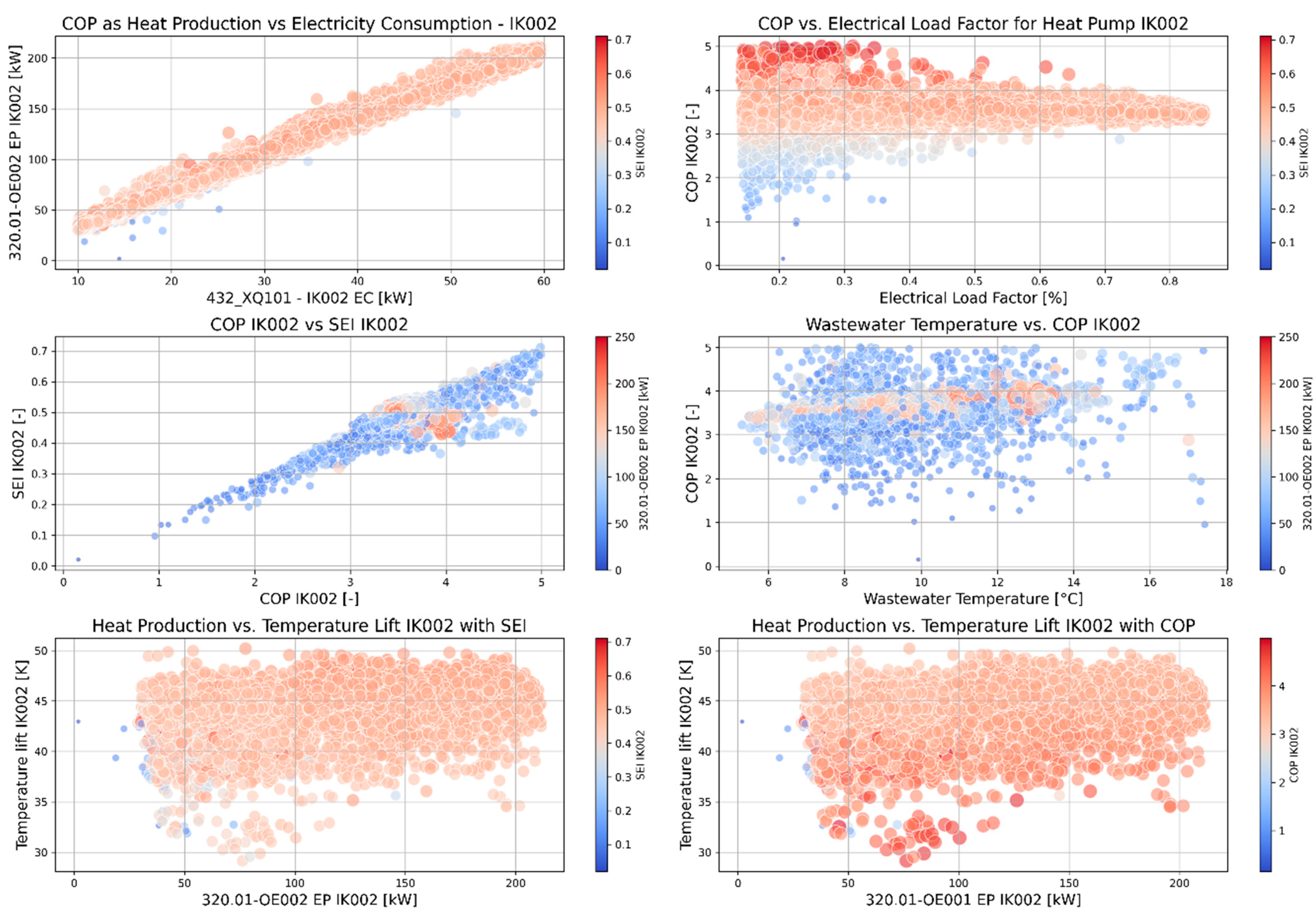
4.1. Wastewater as a Thermal Reservoir: Evaluating Temperature and Other Influences on Heat Pump Performance

The results show that the operational SCOP of the heat pump system met the initial design targets in both evaluated years, indicating that the system is functioning as intended. This section delves deeper into the factors influencing the efficiency of the heat pump system, focusing on both the Coefficient of Performance (COP) and System Efficiency Indicator (SEI). The aim is to identify which parameters most significantly affect the COP and to assess the resulting SEI, determining if, despite satisfactory COP figures on paper, there is room for improvement or specific operational conditions that notably improve or weaken the SEI.
The most significant factors influencing the COP of a building heat pump system are the temperature lift between the heat source and sink and performance variations during part-load conditions, both of which fluctuate with seasonal and ambient temperature changes [47]. To analyze these influences, correlation matrices for relevant parameters were developed using Pearson’s correlation [41]. The parameters analyzed include Wastewater Temperature, Electrical Load Factor (ELF), Temperature Lift, COP, and SEI. The correlation matrices in Figure 17 provide detailed insights into the operations of heat pump systems IK001 and IK002. Specifically:
IK001: A weak correlation (−0.08) between COP and SEI indicates that COP alone does not fully reflect the system’s efficiency. It is a well-established principle in heat pump theory that an increase in temperature lift leads to a decrease in COP. When the ambient temperatures are low, the wastewater temperature generally decreases as well (see Section 4.4 for further details). Under colder ambient conditions, the setpoint temperature for heat distribution is typically at its highest. This scenario, coupled with low source temperature, results in a greater temperature lift between the condenser and evaporator. The inverse relationship between COP and temperature lift is demonstrated in practice by a correlation of −0.84.
Additionally, a negative correlation between the ELF and wastewater temperature indicates that the heat pump operated at higher capacities at lower source temperatures, consuming more energy. This expected behavior reflects how the heat pumps typically respond to increased heating demands during colder periods. Despite higher energy usage and lower COP when the ELF was high, a positive correlation between the ELF and SEI suggests that the heat pump may still achieve higher efficiency when operating close to maximum capacity.
IK002: The correlation matrix for heat pump IK002 requires careful interpretation, as this unit has been significantly less active compared to IK001, often serving primarily as a peak heater with brief periods of operation. To prevent bias in the analysis from the unit’s frequent start-stop cycles, all data points with energy consumption below 10 kW were removed, leaving a dataset of 6566 rows for analysis. This filtering process affects the robustness of data correlations.
For this heat pump, SEI and COP were strongly correlated, with a coefficient of 0.84, contrasting sharply with IK001. This unit’s COP showed less sensitivity to variations in temperature lift, wastewater temperature, and ELF compared to IK001.
To provide a deeper understanding of how each heat pump operates, scatter plots between relevant parameters have been created, with a color index highlighting key trends. These are presented for heat pumps IK001 and IK002 in Figure 18 and Figure 19, respectively. These visuals help illustrate the correlations discussed earlier, demonstrating the dynamic relationships between variables such as COP, ELF, and wastewater temperature at various operational conditions of the heat pumps.
Observations from the correlation matrix and scatter plots provide detailed insights into the operational dynamics of the heat pumps. Since IK001 has significantly more stable operation data, it serves as a more reliable benchmark for evaluating overall system performance and identifying optimal operational strategies.
For both heat pumps, the relationship between heat production and electricity consumption is represented as a near-linear line, seen in the upper left figure, with the slope of the line indicating COP. A slight change in the slope, as heat production increases, suggests a minor decrease in COP at higher production levels.
In the case of IK001, plotting COP against the ELF with SEI as the color index reveals that, while COP decreases with increasing Electrical Load Factor, the SEI remains above 0.45, indicating excellent operation when the ELF is above 40%. Even at 20–40% ELF, the SEI stays within the ‘good’ range most of the time.
This trend is further confirmed in the middle-left figure, which plots SEI vs. COP, with heat production as the color index. For IK001, two distinct patterns emerge: a linear-shaped relationship, represented by a blue line at lower heat production, and a concentrated cluster of red dots at higher heat production levels. This suggests that the heat pump performs more efficiently at higher capacity. Both heat pumps are equipped with four semi-hermetic stable compressors: two are controlled by inverters and two operate on an on/off basis. When the capacity exceeds a certain threshold, both on/off compressors are activated, and the inverter-controlled compressors adjust to fine-tune the production. The blue line likely represents periods when only the inverter-controlled compressors are operating, while the red dots indicate periods where at least one of the on/off compressors is running, consistently achieving excellent SEI values. For IK002, this pattern is less obvious due to fewer data points. However, when energy production is high, both COP and SEI remain above the thresholds for optimal operation. The SEI vs. COP scatter plots illustrate different correlation patterns for the two heat pumps. IK001 displays a more complex pattern, with a linear relationship at lower capacities and a more stable pattern at higher capacities. In contrast, IK002, having fewer data points at high capacity, shows a trend closer to linear. This simpler pattern explains why the correlation between SEI and COP is stronger for this heat pump.
The right-side middle figures plot COP against wastewater temperature, with heat production serving as the color code. The chart consistently shows COP values above 3.0, confirming that the system has operated within expected levels. For IK001, the parts of the data form a red pattern resembling a rotated ellipse, highlighting high-capacity operations. At lower temperatures around 5 °C, COP is about 3.2–3.3. As wastewater temperature increases to around 13 °C, COP peaks at 3.6. Beyond this temperature, as capacities decrease, COP varies more. The plot suggests that lower wastewater temperatures, while significant, do not directly correlate with the lowest COP values, likely because these figures do not account for temperature lift. The bottom figures, which plot Energy Production against Temperature Lift with SEI and COP as color indices, show that temperature lift significantly influences COP: higher production with lower temperature lift results in higher COP. Additionally, these figures demonstrate the differences between SEI and COP, indicating that while COP decreases, SEI values generally increase with higher temperature lifts, signaling more efficient operation at higher lifts.
Overall, with COP values mostly above 3.0 and SEI values above 0.4, the system’s operation ranges from good to excellent. Even though COP decreases at high production levels, this is expected due to the higher temperature lifts involved. The main challenge appears to be the uneven operation between IK001 and IK002, where IK002 is less efficient than IK001, mainly due to its frequent starts and stops. Adjusting the operational hours of the machines, with IK001 operating less and IK002 more, could potentially extend the system’s lifespan and improve overall efficiency. This adjustment can be explored manually by changing the setpoint in the control system or as part of an academic modeling exercise. The wastewater heat exchanger system performs as anticipated, contributing to the strong COP and SEI values, even at the lowest wastewater temperatures.

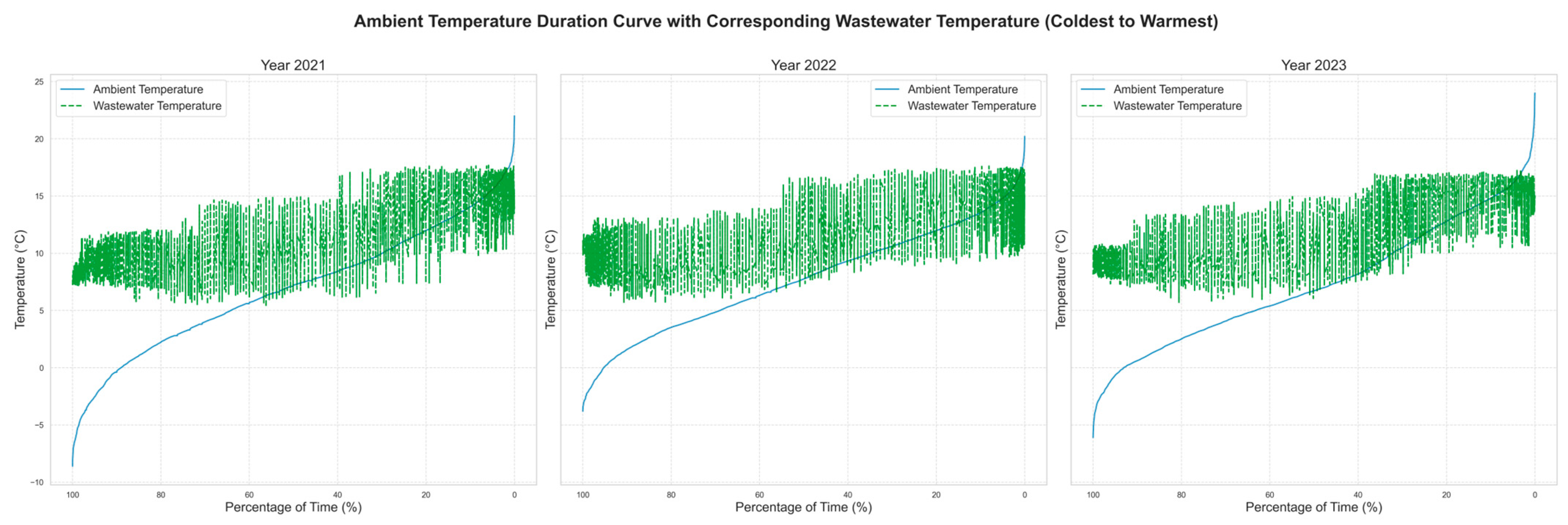
4.2. Comparing Wastewater and Ambient Air as Thermal Reservoirs

To evaluate wastewater as a thermal reservoir, its temperature is compared to the corresponding ambient air temperatures. Historical data for wastewater temperature from 2021 to 2023 is shown on the top in Figure 20, displaying a clear seasonal pattern. The lowest temperatures occur in winter and the highest in summer, aligning with the estimated temperature ranges used for system design.
In the bottom, Figure 20 presents a time series from January 2021 to December 2023, showcasing both wastewater and ambient temperatures. Figure 21 plots the duration curve for each year’s ambient temperature alongside the corresponding wastewater temperature for the same hours. These visualizations clearly demonstrate that the wastewater temperature is generally more stable than the ambient temperature.
A correlation analysis between wastewater and ambient air temperatures reveals a strong positive relationship, with correlations of 0.79 for 2021, 0.73 for 2022, and 0.80 for 2023. These values suggest that as ambient temperatures rise or fall, wastewater temperatures generally follow. Despite the clear correlation, Figure 21 shows the significant stability of wastewater temperatures. For instance, even as the ambient temperature drops to nearly −10 °C, the wastewater temperature never falls below +5 °C. The wastewater temperature remains stable because it mixes stormwater with warmer household wastewater and continuously flows through an underground tunnel insulated by surrounding rocks. The duration curves further highlight the advantage of wastewater compared to ambient air, consistently showing that wastewater temperatures remain higher than ambient air when there is a demand for heat and lower when cooling is required.

4.3. ANN for Monitoring and Evaluating the Heat Pump System and Fouling

Previously, results from both visual validation and test data analysis of the ANN representing the heat pump system were reported. The visual validation identified periods of high error, particularly in the initial days and notably on 12 November. Closer examination during these times indicated that the errors originated from a malfunction in one of the compressors of heat pump IK001. This discovery led to refining the data cleaning criteria, removing similar erroneous data points from the final training dataset. Utilizing a dataset that extends beyond standard validation or test sets, an approach not typical in conventional machine learning practices, provided the flexibility to adjust the dataset based on domain knowledge.
In the unseen test set, the results of the ANN model demonstrate a MAPE of about 5% for heat production and electricity consumption and 0.5% for the outlet temperature for most of the test period, which is considered satisfactory. However, an exception occurs during a four-day period, 21 February 2024 to 25 February 2024, where the errors are significantly higher. A potential issue can be assumed by investigating the input data in Figure 13, which shows that the inlet temperature is noticeably lower than during other periods.
The ANN model was designed to correlate wastewater temperature and inlet conditions with the combined production and consumption of the two heat pumps. By plotting a time series of the output from each heat pump separately, along with the gas boiler contribution, as shown in Figure 22, the source of these errors in predictions becomes clearer. Normally, heat pump IK001 operates as the base load unit, while IK002 has a peak load functionality. However, during the specific four-day period, IK001 was shut off, likely due to a malfunction or scheduled maintenance. Consequently, IK002 automatically took over as the base load unit. Since IK002 is set to produce a temperature 5 K lower than that of IK001, the resulting outlet temperature was lower than normal. This affected the inlet temperature of the heat pumps and caused the gas boiler to compensate. This led to increased usage of expensive gas, even though IK002 had the capacity to meet a larger share of the demand.
A significantly higher prediction error during faulty operation is expected since similar data were excluded from the training dataset. This scenario demonstrates the model’s ability to detect operations that deviate from expected behavior, highlighting potential issues. Had there been an actual malfunction, the system would have triggered an immediate alarm, and while a model trained on hourly data does not support real-time monitoring, the model is robust enough to identify unusual operational patterns, which enhances the data cleaning beyond manual methods. This is particularly useful when retraining the model with a larger dataset, making it a practical tool for proactive maintenance and efficient management.
When assessing whether any significant fouling has occurred between the training data from 2020 to 2022 and the testing data from 2024, the low error rates on the healthy operational data suggest that the system’s capability of extracting heat from the wastewater has remained stable. Despite the test data being from the period of typically low wastewater temperatures, the model’s performance in 2024 reflects similar patterns observed in previous years. It should be noted that the error rates for the test set are higher than those from the visual validation but still fall within an acceptable range, indicating no significant fouling issues. Since the visual validation set was actively used to refine the model and dataset, lower error rates in this set, compared to the test set, are expected.
The ANN is specifically trained on fixed operational conditions. Significant changes in this study case system, such as variations in the setpoint regime of the heat pumps or modifications to the circulation pump control, would affect the model’s reliability. The robustness of the ANN validated between 2020 and 2024 depends on its training under stable operational conditions. While ANNs and deep learning systems are capable of processing and learning from large datasets, they require ongoing monitoring and retraining to adapt to new operational conditions.
Furthermore, in a scenario where fouling does occur in the heat exchangers, the ANN’s predictions would likely deviate as heat extraction efficiency decreases. Rather than training the model on fouling data, it would be preferable to initiate actions to improve operation and prevent or address fouling effectively.

4.4. Assessing Wastewater as a Thermal Reservoir from the Perspective of the Municipal Energy Plant Project

The evaluation of temperature conditions within the wastewater system and its significant contribution to heat pump production demonstrate that wastewater is a stable and predictable low-temperature reservoir suitable for both heating and cooling. The ANN modeling suggests minimal impact from fouling over the years, confirming the supplier’s claims from the design and installation phases.
The major challenges in replicating a similar project involve accessing the wastewater, both physically and through regulatory means. The regulatory issues include ownership rights, permissions for installation, and requirements from the wastewater treatment company. In this project, the wastewater tunnel is owned by the municipality, simplifying ownership discussions compared to many other projects. If a private building were to use a public wastewater tunnel, there is potential for a charge for accessing the low-temperature energy, making the system less appealing. A significant challenge was the need to reroute the wastewater flow during installation, which involved temporarily discharging it untreated into the sea. This action required approval from county management, which was granted without major objections but required a detailed plan outlining the duration of the installation phases. The project calculations indicated a maximum temperature drop in the wastewater of about 0.5 K, a change considered negligible from the perspective of wastewater operators. However, the temperature of the wastewater entering the treatment plant remains a critical factor, potentially a dealbreaker for larger implementations.
Accessing the installation site within the wastewater system was challenging, as the nearest entry point was about 1 km from the actual installation site. A small electric vehicle was employed to transport the 108 plates, each weighing 100 kg, through the tunnel. Before transportation could begin, approximately 75,000 kg of accumulated dirt at the entry point of the tunnel had to be cleared, delaying installation by a week, increasing costs, and extending the period of untreated wastewater discharge. Working far away from the nearest exit in a confined and isolated space significantly heightened safety concerns, leading to strict evacuation procedures, gas detection measures, and the provision of a small rubber boat for emergency use.
The transportation and installation of the heat exchangers began on a Monday morning and concluded by Thursday evening. The highly trained team worked 15–16 h per day to speed up the process and minimize the untreated wastewater discharge period, likely also motivated by a desire to reduce their time at the site.
The drilling process was challenging, requiring precise alignment of three tunnels to hit the wall of the wastewater tunnel, 100 m away. This phase of the project received bids from only one drilling company, resulting in significantly higher costs than anticipated and impacting the overall budget.
A preliminary life-cost analysis compared the Levelized Cost of Energy (LCOE) for this wastewater system with those of geothermal and seawater heat pump systems. While the performance of the wastewater system was comparable to these alternatives, the significant costs associated with drilling and dirt removal did raise the overall installation costs. Nevertheless, the project is regarded as a success by the Municipality of Stavanger. It met the objectives of the EU project within the estimated budget, and importantly, the most uncertain aspect, utilizing wastewater as a heat source, has operated flawlessly.
A significant challenge for the long-term performance and reliability of the system is accessing the heat exchangers. As humorously highlighted in Figure 23 with a “see you later” sign left at the tunnel exit by the installers, the system is located 1000 m away, sealed within the wastewater tunnel. There is no straightforward means for re-access. Although the system is designed to be maintenance-free on paper, the difficulty of accessing it poses real challenges in the event of a malfunction. Accessing the system would require shutting down the wastewater tunnel again, disrupting water transportation and releasing the untreated wastewater into the sea.
Moreover, the custom design of the heat exchangers and the challenging conditions at the installation site significantly complicate the replacement or repair of malfunctioning elements. The energy plant is equipped with full backup options for heat production, allowing for potential shutdowns during the winter season, if necessary. However, these interventions are complex and require careful planning and consideration, with increased operational costs as well as the cost of the new equipment. Notably, if there is no backup for cooling and a malfunction occurs in the heat exchanger system, it could lead to significant comfort issues during the summer.

5. Conclusions

This study has presented a detailed description and analysis of an advanced wastewater heat pump system for heating and cooling production. The system’s performance was evaluated, and an ANN was employed to model the heat pump operations, confirming minimal deterioration due to fouling over the last four years. Key conclusions from this study include the following:
  • The project is considered successful by those responsible for its specification, design, and operation, despite substantial challenges. The wastewater system has proven to be an effective thermal reservoir, maintaining higher temperatures than ambient air during winter for heating operations and colder temperatures during summer for cooling. The consistent temperature stability, never dropping below +5 °C, ensures a reliable heat source during the coldest days. Additionally, the innovative design of the wastewater heat exchanger plates, which are flexible and adaptable to various configurations, makes them ideal for both new and existing wastewater systems.
  • There is room to improve the control strategy of the two heat pumps. Notably, heat pump IK001, which operates more frequently than IK002, achieves a higher SCOP despite being set to produce heat at a higher temperature. Re-evaluating the setpoint scheme is recommended, possibly through manual adjustments or by using the ANN model for optimization.
  • The ANN has confirmed that the heat exchangers have not experienced degradation due to fouling. Moreover, it has effectively identified operational errors, pinpointing areas for improvement in heat pump management. This demonstrates the model’s utility in guiding operational adjustments. Integrating physics-based modeling with the ANN could further enhance the model’s operational range.
  • The main challenges associated with the technology involve accessing the wastewater, addressing issues of ownership, tariffs, and wastewater temperature before it reaches the treatment plant, in addition to the physical installation and establishment of the wastewater heat pump system.
  • Future work on this project could aim to refine the control systems of the heat pumps and develop an enhanced fault detection mechanism. Using information from the current manual maintenance logs, more detailed information on the sources of heat pump faults could be extracted and utilized within the machine learning framework. The analysis clearly indicates that the system lacks an automatic response to correct errors as they occur, leading to subsequent issues in other parts of the plant. Therefore, developing a methodology that combines practical knowledge with ML could be a valuable direction for future research.
  • Looking ahead more broadly, future studies could investigate the utilization of wastewater as a thermal resource within urban planning, promoting the development of larger integrated systems that utilize this sustainable energy source.

Author Contributions

Conceptualization, F.S.F. and M.A.; methodology, F.S.F.; validation, F.S.F.; formal analysis, F.S.F.; data curation, F.S.F.; writing—original draft preparation, F.S.F.; writing—review and editing, M.A.; visualization, F.S.F.; supervision, M.A.; project administration, F.S.F.; funding acquisition, F.S.F. and M.A. All authors have read and agreed to the published version of the manuscript.

Funding

This research was partially funded by the Norwegian Research Council (project 311269) and Norconsult Norge AS (project 5195400).

Data Availability Statement

The data presented in this study are available on request to the corresponding author.

Acknowledgments

The authors would like to thank the municipal representative in Stavanger for discussions, access to data, and advice. The authors appreciate the feedback and suggestions received from colleagues and friends. The OpenAI GPT-4 model was employed for editorial assistance.

Conflicts of Interest

Author F.S.F. is employed by the Norwegian Consultant Engineering Company, Norconsult Norge AS, which partly funds his industrial Ph.D. project. The remaining author declares that research was conducted in the absence of any commercial or financial relationships that could be construed as potential conflicts of interest.

Abbreviations

AIArtificial Intelligence
ANNArtificial Neural Network
COPCoefficient of Performance
DHWDomestic Hot Water
EEREnergy Efficiency Ratio
ELFElectrical Load Factor
IEAInternational Energy Agency
IK001Identifier for the first heat pump in the system
IK002Identifier for the second heat pump in the system
LCOELevelized Cost of Energy
MAEMean Absolute Error
MAPEMean Absolute Percentage Error
MLMachine Learning
MEG2020% Monoethylene Glycol solution
OECDOrganization for Economic Co-operation and Development
ReLURectified Linear Unit
RSMERoot Mean Square Error
SCADASupervisory Control and Data Acquisition
SCOPSeasonal Coefficient of Performance
SEISystem Efficiency Index
SPFSeasonal Performance Factor
Symbols and Variables
c p Specific Heat Capacity (in kJ/kgK)
m Mass flow rate (in kg/s)
Q ˙ Rate of heat transfer (in kW)
rPearson’s correlation coefficient
TTemperature
W ˙ h p Electrical input to the heat pump (in kWh/h)

References

  1. IEA. Empowering Cities for a Net Zero Future: Unlocking Resilient, Smart, Sustainable Urban Energy Systems; IEA: Paris, France, 2020. [Google Scholar]
  2. IEA. Net Zero by 2050; IEA: Paris, France, 2021. [Google Scholar]
  3. IEA. Heat Pumps; IEA: Paris, France, 2020. [Google Scholar]
  4. Byrne, P. Modelling and Simulation of Heat Pumps for Simultaneous Heating and Cooling, a Special Issue. Energies 2022, 15, 5933. [Google Scholar] [CrossRef]
  5. Rosenow, J.; Gibb, D.; Nowak, T.; Lowes, R. Heating up the global heat pump market. Nat. Energy 2022, 7, 901–904. [Google Scholar] [CrossRef]
  6. Madani, H.; Claesson, J.; Lundqvist, P. Capacity control in ground source heat pump systems. Int. J. Refrig. 2011, 34, 1338–1347. [Google Scholar] [CrossRef]
  7. Lund, R.; Persson, U. Mapping of potential heat sources for heat pumps for district heating in Denmark. Energy 2016, 110, 129–138. [Google Scholar] [CrossRef]
  8. Blázquez, C.S.; Nieto, I.M.; García, J.C.; García, P.C.; Martín, A.F.; González-Aguilera, D. Comparative Analysis of Ground Source and Air Source Heat Pump Systems under Different Conditions and Scenarios. Energies 2023, 16, 1289. [Google Scholar] [CrossRef]
  9. Klein, K.; Huchtemann, K.; Müller, D. Numerical study on hybrid heat pump systems in existing buildings. Energy Build. 2014, 69, 193–201. [Google Scholar] [CrossRef]
  10. Carroll, P.; Chesser, M.; Lyons, P. Air Source Heat Pumps field studies: A systematic literature review. Renew. Sustain. Energy Rev. 2020, 134, 110275. [Google Scholar] [CrossRef]
  11. IEA. The Future of Heat Pumps; IEA: Paris, France, 2022. [Google Scholar]
  12. Nagpal, H.; Spriet, J.; Murali, M.; McNabola, A. Heat Recovery from Wastewater—A Review of Available Resource. Water 2021, 13, 1274. [Google Scholar] [CrossRef]
  13. Patil, V.; Kadam, A. Problems and Perspectives of the Urban Sewage System: A Geographical Review. Res. Rev. Int. J. Multidiscip. 2019, 4, 2815–2819. [Google Scholar]
  14. Culha, O.; Gunerhan, H.; Biyik, E.; Ekren, O.; Hepbasli, A. Heat exchanger applications in wastewater source heat pumps for buildings: A key review. Energy Build. 2015, 104, 215–232. [Google Scholar] [CrossRef]
  15. Klimaetaten Oslo. Bringing You Heat That’s Been Extracted from Your Sewage. Available online: https://www.klimaoslo.no/district-heating-from-sewage/ (accessed on 28 May 2024).
  16. Seehus, G.; Vigre, E. What Is Triangulum? Available online: https://triangulum.no/about-triangulum/?lang=en (accessed on 21 July 2024).
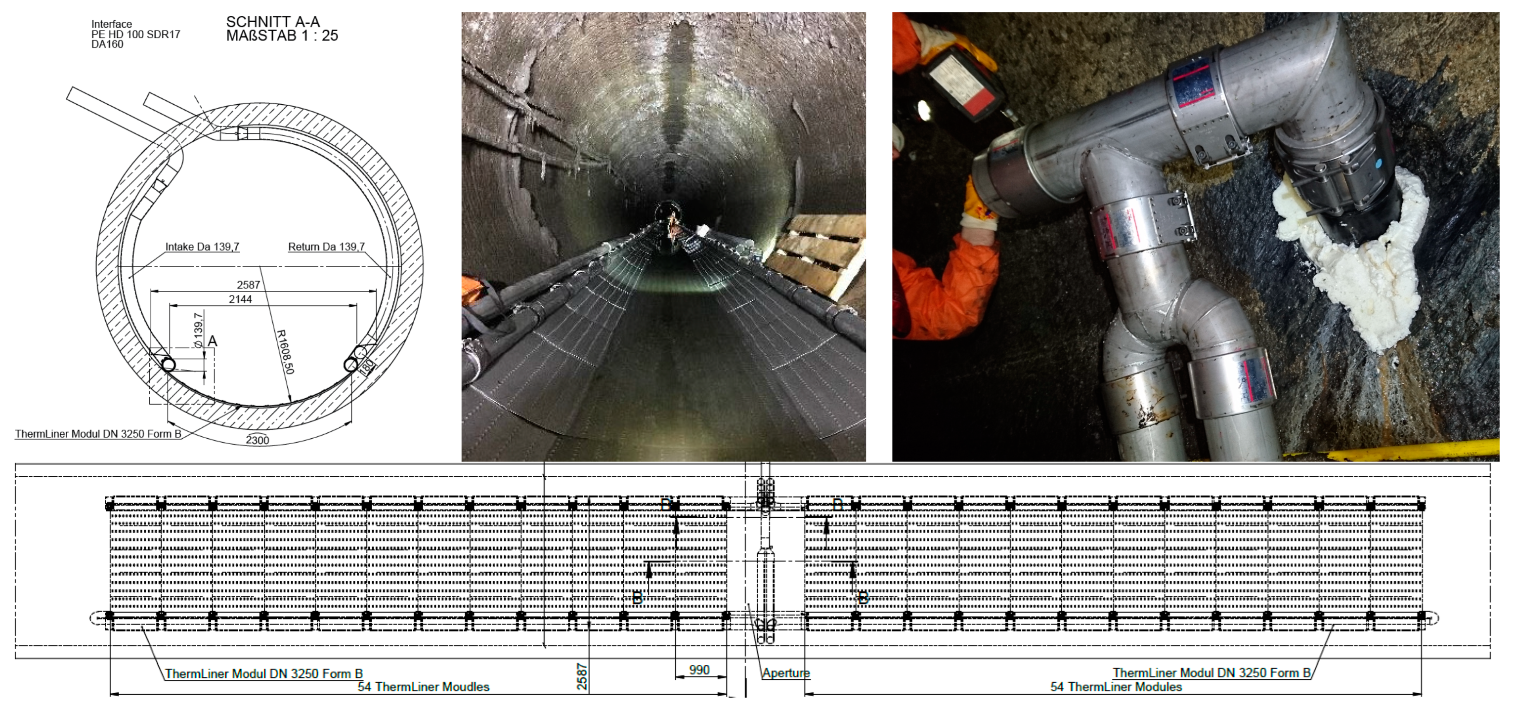
  17. Helmut UHRIG Straßen- und Tiefbau GmbH. UHRIG Product: Therm-Liner. 2020. Available online: https://www.uhrig-bau.eu/en/division/heat-from-wastewater/product-therm-liner/ (accessed on 21 July 2024).
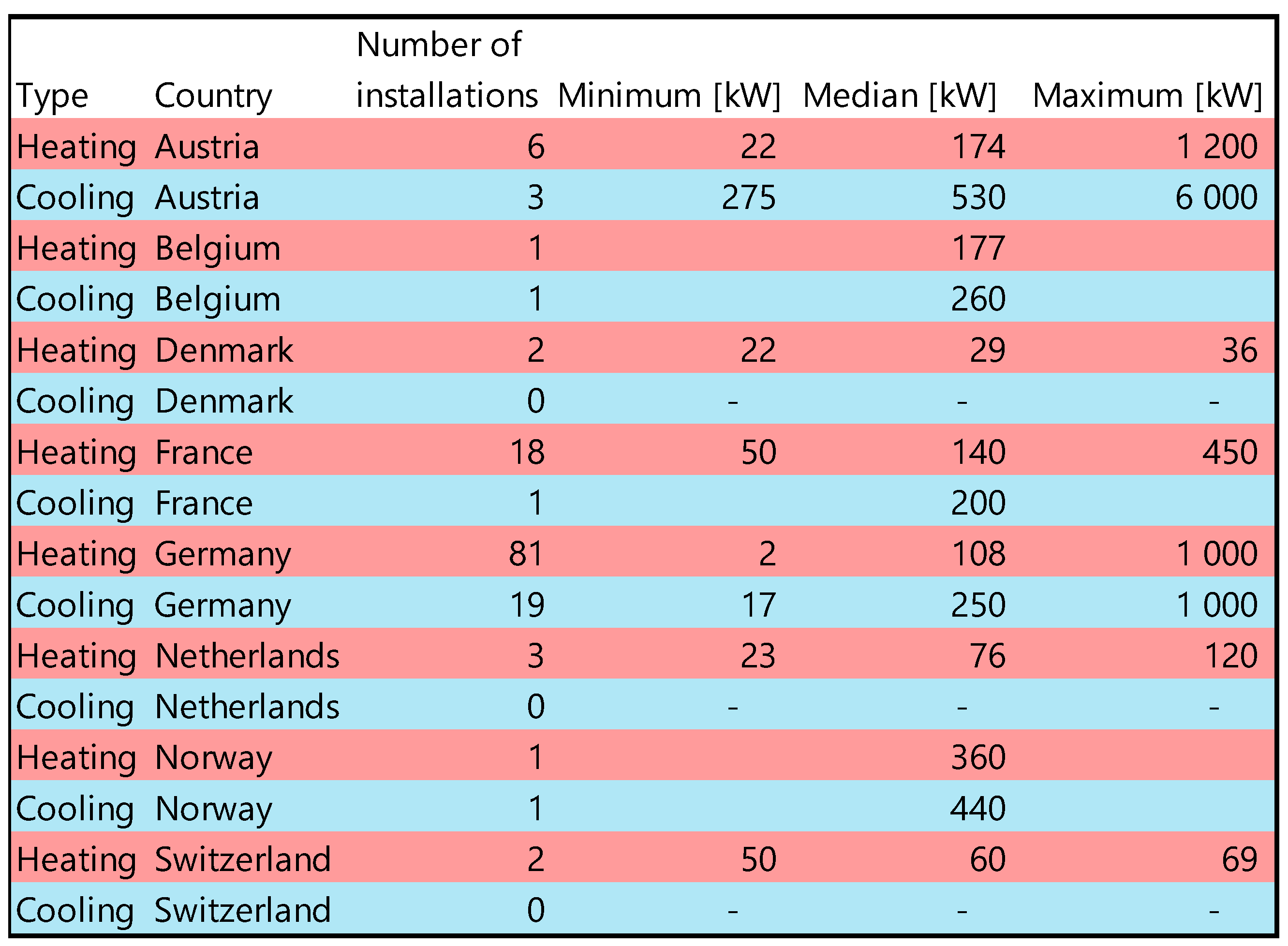
  18. Helmut UHRIG Straßen- und Tiefbau GmbH. References UHRIG Energy from Wastewater, Therm-Liner, Last Update: 31.03.2023. Available online: https://www.uhrig-bau.eu/wp-content/uploads/2020/11/230331-references-uhrig-energy-from-wastewater.pdf (accessed on 21 July 2024).
  19. Bartnicki, G.; Ziembicki, P.; Klimczak, M.; Kalitka, A. The Potential of Heat Recovery from Wastewater Considering the Protection of Wastewater Treatment Plant Technology. Energies 2022, 16, 227. [Google Scholar] [CrossRef]
  20. Kowalik, R.; Bąk-Patyna, P. Analysis of Heat Recovery from Wastewater Using a Heat Pump on the Example of a Wastewater Treatment Plant in the ŚwiĘtokrzyskie Voivodeship in Polish. Struct. Environ. 2021, 13, 90–95. [Google Scholar] [CrossRef]
  21. Łokietek, T.; Tuchowski, W.; Leciej-Pirczewska, D.; Głowacka, A. Heat Recovery from a Wastewater Treatment Process—Case Study. Energies 2022, 16, 44. [Google Scholar] [CrossRef]
  22. Cecconet, D.; Raček, J.; Callegari, A.; Hlavínek, P. Energy Recovery from Wastewater: A Study on Heating and Cooling of a Multipurpose Building with Sewage-Reclaimed Heat Energy. Sustainability 2019, 12, 116. [Google Scholar] [CrossRef]
  23. Aprile, M.; Scoccia, R.; Dénarié, A.; Kiss, P.; Dombrovszky, M.; Gwerder, D.; Schuetz, P.; Elguezabal, P.; Arregi, B. District Power-To-Heat/Cool Complemented by Sewage Heat Recovery. Energies 2019, 12, 364. [Google Scholar] [CrossRef]
  24. Xu, T.; Wang, X.; Wang, Y.; Li, Y.; Xie, H.; Yang, H.; Wei, X.; Gao, W.; Lin, Y.; Shi, C. Integration of sewage source heat pump and micro-cogeneration system based on domestic hot water demand characteristics: A feasibility study and economic analysis. Process Saf. Environ. Prot. 2023, 179, 796–811. [Google Scholar] [CrossRef]
  25. Chen, W.-A.; Lim, J.; Miyata, S.; Akashi, Y. Methodology of evaluating the sewage heat utilization potential by modelling the urban sewage state prediction model. Sustain. Cities Soc. 2022, 80, 103751. [Google Scholar] [CrossRef]
  26. Aguilera, J.J.; Meesenburg, W.; Markussen, W.B.; Zühlsdorf, B.; Elmegaard, B. Real-time monitoring and optimization of a large-scale heat pump prone to fouling—Towards a digital twin framework. Appl. Energy 2024, 365, 123274. [Google Scholar] [CrossRef]
  27. Meesenburg, W.; Aguilera, J.J.; Kofler, R.; Markussen, W.B.; Brian, E. Prediction of fouling in sewage water heat pump for predictive maintenance. In Proceedings of the 35th International Conference on Efficiency, Cost, Optimization, Simulation and Environmental Impact of Energy Systems 2022, Copenhagen, Denmark, 3–7 July 2022. [Google Scholar]
  28. Zhuang, Z.; Zhao, J.; Mi, F.; Zhang, T.; Hao, Y.; Li, S. Application and Analysis of a Heat Pump System for Building Heating and Cooling Using Extracting Heat Energy from Untreated Sewage. Buildings 2023, 13, 1342. [Google Scholar] [CrossRef]
  29. Wang, J.; Sun, L.; Li, H.; Ding, R.; Chen, N. Prediction Model of Fouling Thickness of Heat Exchanger Based on TA-LSTM Structure. Processes 2023, 11, 2594. [Google Scholar] [CrossRef]
  30. Kim, M.-H.; Kim, D.-W.; Han, G.; Heo, J.; Lee, D.-W. Ground Source and Sewage Water Source Heat Pump Systems for Block Heating and Cooling Network. Energies 2021, 14, 5640. [Google Scholar] [CrossRef]
  31. Helmut UHRIG Straßen- und Tiefbau GmbH. Energy from Wastewater with UHRIG Therm-Liner Description of the Heat Exchanger System. Available online: https://www.uhrig-bau.eu/wp-content/uploads/2021/04/en-system-description-uhrig-energy-from-wastewater-eu-211210-1.pdf (accessed on 21 July 2024).
  32. OECD. Measuring Smart Citities Performance; OECD: Paris, France, 2020. [Google Scholar]
  33. Fadnes, F.S.; Olsen, E.; Assadi, M. Holistic management of a smart city thermal energy plant with sewage heat pumps, solar heating, and grey water recycling. Front. Energy Res. 2023, 11, 1078603. [Google Scholar] [CrossRef]
  34. Zou, J.; Hirokawa, T.; An, J.; Huang, L.; Camm, J. Recent advances in the applications of machine learning methods for heat exchanger modeling—A review. Front. Energy Res. 2023, 11, 1294531. [Google Scholar] [CrossRef]
  35. Starzec, M.; Kordana-Obuch, S.; Piotrowska, B. Evaluation of the Suitability of Using Artificial Neural Networks in Assessing the Effectiveness of Greywater Heat Exchangers. Sustainability 2024, 16, 2790. [Google Scholar] [CrossRef]
  36. Çengel, Y.A. Heat and Mass Transfer: A Practical Approach, 3rd ed.; McGraw-Hill Science Engineering: Blacklick, OH, USA, 2006. [Google Scholar]
  37. DKRT. Om DKRT—Dansk Kloak RenoveringsTeknik ApS. Available online: https://kloakshop.dk/om-os/ (accessed on 21 July 2024).
  38. Schneider Electric. Citect SCADA 2018 Installation and Configuration Guide; Schneider Electric: Rueil-Malmaison, France, 2018. [Google Scholar]
  39. Andresen, T.; Nekså, P.; Stene, J. Heat Pumps in Smart Energy-Efficient Buildings A State-of-the-Art Report; NTNU and SINTEF: Trondheim, Norway, 2002. [Google Scholar]
  40. Lane, A.-L.; Benson, J.; Eriksson, L.; Fahlén, P.; Nordman, R.; Haglund Stignor, C.; Berglöf, K.; Hundy, G. Method and Guidelines to Establish System Efficiency Index during Field Measurements on Air Conditioning and Heat Pump Systems; SP Technical Research Institute of Sweden: Borås, Sweden, 2014. [Google Scholar]
  41. Géron, A. Hands-On Machine Learning with Scikit-Learn, Keras, and TensorFlow, 2nd ed.; Tache, R.R.a.N., Ed.; O’Reilly Media, Inc.: Sebastopol, CA, USA, 2019. [Google Scholar]
  42. Abida, A.; Richter, P. HVAC control in buildings using neural network. J. Build. Eng. 2023, 65, 105558. [Google Scholar] [CrossRef]
  43. Fadnes, F.S.; Banihabib, R.; Assadi, M. Using Artificial Neural Networks to Gather Intelligence on a Fully Operational Heat Pump System in an Existing Building Cluster. Energies 2023, 16, 3875. [Google Scholar] [CrossRef]
  44. Witte, R.S.W.; John, S. Statistics, 11th ed.; John Wiley & Sons, Inc.: Hoboken, NJ, USA, 2017. [Google Scholar]
  45. Russo, R. Stop Using Moving Average to Smooth Your Time Series; BIP xTech: Rome, Italy, 2024. [Google Scholar]
  46. de Myttenaere, A.; Golden, B.; Le Grand, B.; Rossi, F. Mean Absolute Percentage Error for regression models. Neurocomputing 2016, 192, 38–48. [Google Scholar] [CrossRef]
  47. Bogdanov, D.; Satymov, R.; Breyer, C. Impact of temperature dependent coefficient of performance of heat pumps on heating systems in national and regional energy systems modelling. Appl. Energy 2024, 371, 123647. [Google Scholar] [CrossRef]
Figure 1. Key figures for the 114 systems installed by UHRIG from 2007 to 2023.
Energies 17 04832 g001
Figure 2. Daily averages of flow, rainfall, and water height in the tunnel (2015). Based on data provided by the municipality of Stavanger.
Energies 17 04832 g002
Figure 3. (Top left) design sketch of the heat exchanger system showing a cross-sectional view. (Top center and right) photographs taken during the system installation. (Bottom) overhead design sketch of the system layout above the tunnel floor. Photos by Uhrig/Municipality of Stavanger.
Energies 17 04832 g003
Figure 4. Thermal energy plant and surrounding buildings in relation to the wastewater tunnel.
Energies 17 04832 g004
Figure 5. Schematic of the energy plant system with relevant sensors and meters.
Energies 17 04832 g005
Figure 6. Model configuration of wastewater heat pump ANN.
Energies 17 04832 g006
Figure 7. Examples of data smoothing using the Savitzky-Golay filter for Heat Production (top), Electricity Consumption (middle) and Wastewater Temperature (bottom).
Energies 17 04832 g007
Figure 8. Duration curve heat production 2022.
Energies 17 04832 g008
Figure 9. Duration curve heat production 2023.
Energies 17 04832 g009
Figure 10. Input values used during visual validation.
Energies 17 04832 g010
Figure 11. Results from visual validation, heat production both heat pumps.
Energies 17 04832 g011
Figure 12. Results from visual validation, outlet temperature from IK001.
Energies 17 04832 g012
Figure 13. Input data for the ANN applied on 2024 test data.
Energies 17 04832 g013
Figure 14. Predicted vs. actual heat production for 2024 test data.
Energies 17 04832 g014
Figure 15. Predicted vs. actual electricity consumption for 2024 test data.
Energies 17 04832 g015
Figure 16. Predicted vs. actual outlet temperature for 2024 test data.
Energies 17 04832 g016
Figure 17. Correlation Matrices for IK001 (top) and IK002 (bottom).
Energies 17 04832 g017
Figure 18. Comprehensive visualization of heat pump performance metrics for IK001, based on 21,800 rows of data. (Top Left) heat production vs. electricity consumption, depicted with a color index representing SEI. (Top Right) COP vs. electrical load factor, with SEI as the color index. (Middle Left) SEI plotted against COP, with heat production serving as the color index. (Middle Right) COP in relation to wastewater temperature, colored by heat production. (Bottom Left) heat production vs. temperature lift with SEI as the color index. (Bottom Right) heat production vs. temperature lift with COP as the color index.
Energies 17 04832 g018
Figure 19. Comprehensive visualization of heat pump performance metrics for IK002, based on 6566 rows of data. Visualizations: same as Figure 18, with datasets corresponding to IK002.
Energies 17 04832 g019
Figure 20. Historical data for the wastewater temperature for the years 2021, 2022, and 2024. Comparison of wastewater temperature and ambient temperature—2021–2023.
Energies 17 04832 g020
Figure 21. Sorted duration curve for ambient temperature with corresponding wastewater temperatures for the years 2021, 2022, and 2023.
Energies 17 04832 g021
Figure 22. Evaluation of heat pump operation during test interval 2024.
Energies 17 04832 g022
Figure 23. A sign mounted on the door entry to the wastewater tunnel by Uhrig, reading “Careful! Heat Exchangers” in Danish.
Energies 17 04832 g023
Table 1. Annual design targets heat pump system in study case.
IndicatorTarget Value
Heat Production Heat Pumps [kWh/yr]1,692,000
Electricity Consumption for Heating [kWh/yr]483,000
Seasonal Coefficient of Performance Heating *3.5
Heat Extraction at Evaporator [kWh/yr]1,209,000
Cooling Production [kWh/yr]187,000
Electricity Consumption for Cooling [kWh/yr]18,700
Seasonal Coefficient of Performance Cooling *10.0
Heat Rejection at Condenser [kWh/yr]205,700
Gas Boiler Contribution Peak Load Heating [kWh/yr]66,000
* Defined in next subchapter.
Table 2. Summary of hyperparameters and training settings for ANN.
ParameterValue
Network Architecture(50, 75, 150)
Activation Functions[‘ReLu’, ‘ReLu’, ‘ReLu’, ‘linear’]
Loss FunctionMean Squared Error
OptimizerAdam
Batch Size150
Epochs5000
Validation Split0.2
Early StoppingEnabled
Patience50
Batch Size150
Save Best ModelYes
Table 3. Accumulated values for plant thermal energy production and energy consumption.
20222023
Energy [kWh/yr]Power [kW]Energy [kWh/yr]Power [kW]
Heat production1,342,0004501,372,000430
Heat Production—IK0011,159,0002441,041,000242
Electricity Consumption—IK001321,00071291,00071
SCOP IK001 [-]3.613.58
Heat Production—IK002177,000231321,000248
Electricity Consumption—IK00252,0006691,00067
SCOP IK002 [-]3.403.52
Heat Pump Production1,336,0004501,362,000430
Electricity consumption373,000131382,000130
SCOP Heat [-]3.583.57
Heat extracted at evaporator Qevap963,000320980,000302.0
Cooling to Heat128,00068123,000118.0
Wastewater Heat835,000304858,000283.0
Gas Boiler Load570019010,000156.0
Cooling Production34,00027044,000233
Electricity Consumption Cooling14,00010015,00081
SEER [-]2.432.93
Electricity Consumption Pumps102,00019110,00019
SPF Total [-]2.782.74
Table 4. Evaluation of visual validation—Error metrics with and without faulty operation.
ParameterMAERMSEMax Absolute ErrorMAPE
Including Errors due to Faulty Operation of IK001
Heat Pump Production [kWh/h]16.334.2157.98.5%
Electricity Consumption [kWh/h]4.39.645.08.5%
Outlet Temperature Heat Pump [°C]0.40.83.55.3%
Excluding Errors due to Faulty Operation of IK001
Heat Pump Production [kWh/h]6.29.224.83.7%
Electricity Consumption [kWh/h]1.82.46.93.3%
Outlet Temperature Heat Pump [°C]0.20.20.60.3%
Table 5. Error metrics for 2024 testing interval, complete and segregated by operational status (without and with faulty operation).
ParameterMAERMSEMax Absolute ErrorMAPE
Complete results including period with significant error.
7 February 2024 to 14 March 2024
Heat Pump Production [kWh/h]33.763.6260.125.8%
Electricity Consumption [kWh/h]9.718.372.626.3%
Outlet Temperature Heat Pump [°C]0.81.56.11.6%
Result excluding period with significant error.
7 February 2024 to 21 February 2024 and 27 February 2024 to 14 March 2024
Heat Pump Production [kWh/h]12.217.0111.65.0%
Electricity Consumption [kWh/h]3.65.138.25.1%
Outlet Temperature Heat Pump [°C]0.30.42.40.5%
Results period with significant error.
21 February 2024 to 27 February 2024
Heat Pump Production [kWh/h]140.4150.7260.1129.4%
Electricity Consumption [kWh/h]40.043.172.6132.2%
Outlet Temperature Heat Pump [°C]3.33.56.17.0%
Disclaimer/Publisher’s Note: The statements, opinions and data contained in all publications are solely those of the individual author(s) and contributor(s) and not of MDPI and/or the editor(s). MDPI and/or the editor(s) disclaim responsibility for any injury to people or property resulting from any ideas, methods, instructions or products referred to in the content.

