An Integrated Frequency Regulation Method Based on System Frequency Security Posture

Abstract

As the share of renewable energy in a grid increases, the grid’s frequency support capability weakens, and the spatial distribution of grid frequency becomes more pronounced. As a result, control strategies based on system frequency consistency and traditional frequency regulation dominated by synchronous machines are becoming increasingly inadequate for meeting the frequency regulation requirements of new-type power systems. To enhance the system’s frequency support capability, it is imperative to fully utilize the frequency regulation resources within the power system. To address this issue, this paper first introduces a system frequency security posture assessment method that accounts for the spatial distribution characteristics of the grid. Subsequently, a parameter optimization method for diverse frequency regulation resources is proposed in conjunction with the proposed comprehensive evaluation method for frequency regulation. Next, using a renewable energy feeder regional grid as an example, an integrated frequency regulation method based on the system frequency security posture is presented. Finally, the frequency regulation performance and economic costs of different frequency regulation methods are analyzed under various operating scenarios and disturbances using a model based on actual data from the renewable energy feeder regional grid. The simulation and index calculation results demonstrate that the method proposed in this paper effectively enhances the system’s frequency support capability, reduces the frequency disparity between different nodes within the grid, and maintains high economic performance.

1. Introduction

With the goal of “building a renewable energy-based power system”, renewable energy units are set to become a primary power source in the future [1,2,3]. Renewable energy units are connected to the power grid through power electronics, which cannot provide reliable frequency support, leading to a decline in system frequency stability. Additionally, the location of renewable energy integration is influenced by geographic factors. This results in an uneven spatial distribution of the system’s frequency regulation sources, consequently leading to greater differences in frequency response among system nodes following a disturbance [4]. The system center frequency index is becoming insufficient for describing the frequency response characteristics of modern power systems. As diversified frequency regulation resources play a more significant role, there is an urgent need for an integrated frequency regulation method that considers the spatial distribution characteristics of system frequency and adapts to the current frequency security posture.

Some scholars have noted that the spatial distribution characteristics of frequency are influenced by factors such as network structure, generator type, and the location of disturbances, becoming more complex as renewable energy penetration increases [5]. To analyze the system’s frequency response more accurately, [6] proposes a method for selecting frequency measurement points based on the center of inertia (COI). However, this approach overlooks the differences between some system nodes and the COI, which can affect the accuracy of frequency response evaluation. In [7], an online identification method for power system inertia distribution is proposed, effectively quantifying the system’s overall inertia and providing a foundation for the subsequent reliable assessment of frequency response. Considering the economic factor of installing frequency monitoring equipment, [8] proposes an inertia estimation method based on generator clustering partitioning. This method reduces the number of frequency monitoring nodes while maintaining estimation accuracy. However, due to the difficulty of obtaining detailed electrical distances between generators in actual large-scale grid models, the engineering practicability is limited. Overall, the research mentioned above primarily focuses on the evaluation of system inertia. Further study is needed on the selection of frequency response measurement nodes based on these evaluations to provide a foundation for enhancing frequency support capability.

Current research on improving system frequency support capability can be broadly classified into two categories: optimizing the unit’s frequency control strategy, and developing allocation and synergy schemes for diversified frequency regulation resources [9,10,11]. To enhance wind turbine frequency regulation, [12] suggests adjusting parameters like the frequency regulation dead zone and droop coefficient. This approach allows for switching between Maximum Power Point Tracking (MPPT) mode and frequency regulation mode, helping to prevent a secondary drop in system frequency. An adaptive control method for wind turbines is proposed in [13], which optimizes the capacity and duration of the turbine’s power response, achieving results comparable to those described above. On the other hand, an adaptive wind-storage cooperative control strategy is proposed in [14], which extends battery life while reducing the capacity of the battery deployment, making it practical for engineering applications. In [15], the frequency regulation sequence of wind power, energy storage, and other resources is configured from the perspective of frequency regulation parameters. The frequency regulation economy is used as an index, and parameter optimization is performed using a multi-objective particle swarm algorithm to provide insights for developing frequency regulation strategies for new-type power systems. In summary, the current system lacks a synergistic scheme for integrating diversified frequency regulation resources. It is crucial to develop an integrated frequency regulation control strategy that leverages the advantages of diversified frequency regulation resources to enhance the system’s frequency support capability.

Proposing reasonable and effective key indexes for system frequency response characteristics is essential for measuring the system’s frequency regulation capability. These indexes are crucial for guiding the optimal allocation and cooperative control of diversified frequency regulation resources. The effectiveness of power system frequency regulation can be assessed from multiple perspectives, including operational reliability, frequency regulation economy, and environmental protection [16,17]. Operational reliability can further be subdivided into two aspects: support power and frequency regulation effectiveness. In [18], the regulation speed, frequency regulation amplitude, state of charge (SOC), and other indexes are selected to evaluate the power support of the energy storage plant from a power perspective. In [19], five indicators—initial frequency rate of change, frequency nadir, transition time, steady-state frequency value, and steady-state time—are selected to evaluate wind power frequency regulation. However, the evaluation is limited to frequency regulation performance, neglecting the economic and environmental impacts. To address these issues, ref. [20] incorporates economic indicators such as investment cost, lifetime cost, and frequency regulation gain into the system’s frequency regulation performance metrics. It is evident that current frequency regulation effectiveness evaluation methods primarily focus on a single type of frequency regulation resource or a single aspect of indexes. Hence, there is a need for a comprehensive evaluation methodology that accommodates the diversity of frequency regulation resources and the multi-dimensionality of evaluation indexes.

In summary, to address the issues of insufficient frequency support capacity and intensified frequency differences across the system’s different regions, this paper proposes an integrated frequency regulation method based on the system frequency security posture. The key contributions of this paper are as follows: (1) A method for assessing system frequency security posture is introduced, considering the spatial distribution characteristics of the grid, which is effective for both system spatial division and security posture assessment. (2) A technique for optimizing the parameters of diversified frequency regulation resources is proposed, grounded in a comprehensive evaluation of the effectiveness of frequency regulation. This technique focuses on optimizing control parameters for frequency regulation resources in a partitioned manner to address frequency distribution disparities arising from the uneven distribution of frequency regulation resources. (3) An integrated frequency regulation approach is developed and validated with a model based on real data from the renewable energy feeder regional grid. This approach enhances the system’s frequency support capability by optimizing each frequency regulation resource’s strengths, meeting the performance, economic, and environmental demands of grid frequency regulation while reducing frequency dispersion.

The content of this paper is organized as follows: Section 2 analyzes system frequency distribution using an actual grid model and proposes a system frequency security posture assessment method that incorporates these spatial characteristics. Section 3 integrates the system frequency security posture, comprehensive effectiveness evaluation of frequency regulation, and parameter optimization methods and proposes a comprehensive frequency regulation approach. Section 4 presents simulations, and Section 5 summarizes the paper.

2. System Frequency Security Posture Assessment Method Considering Spatial Distribution Characteristics

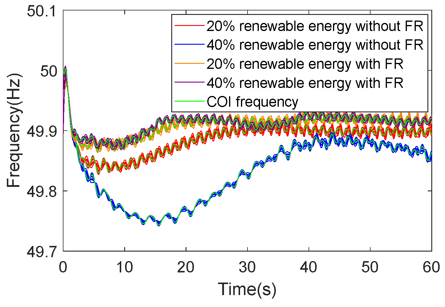
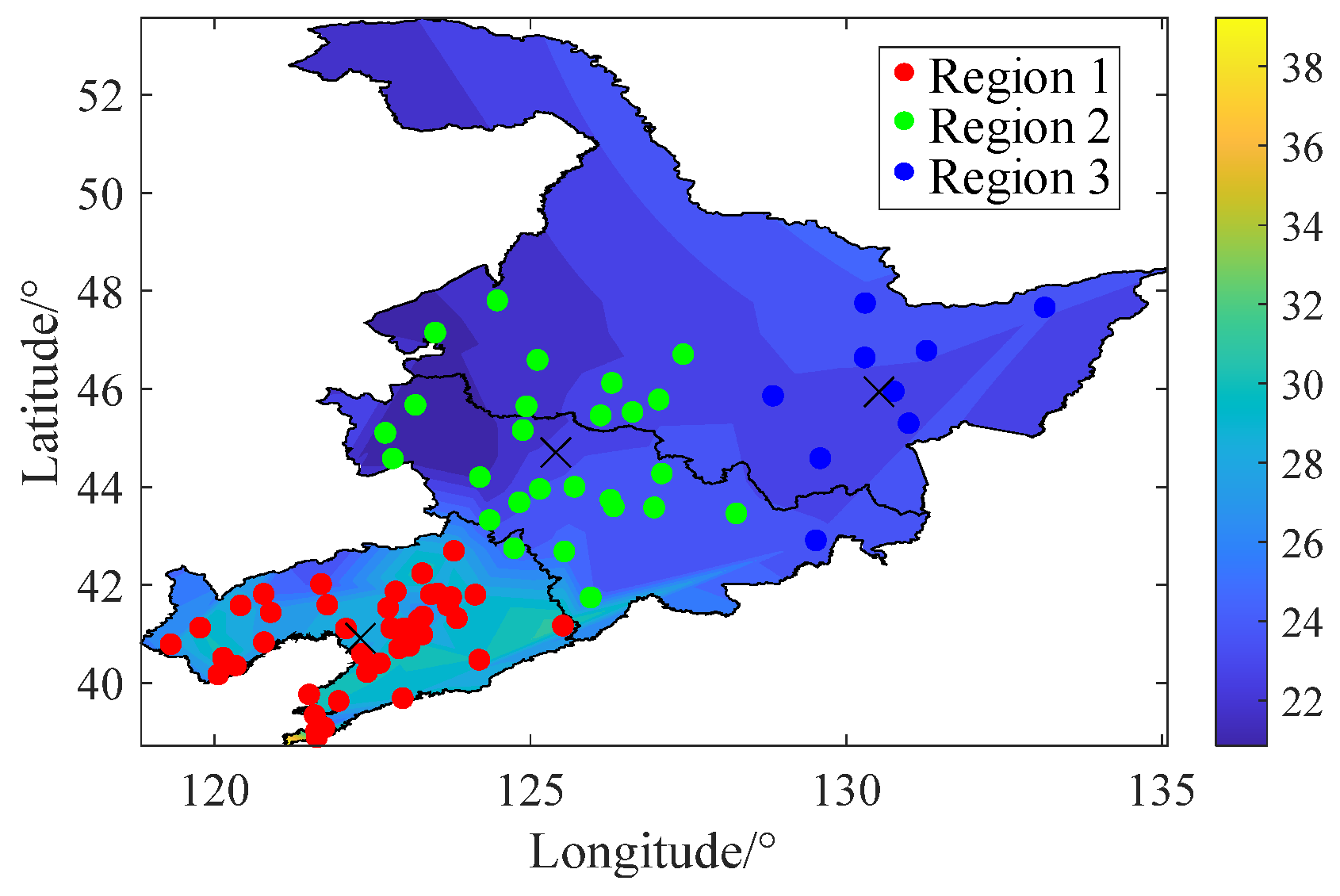
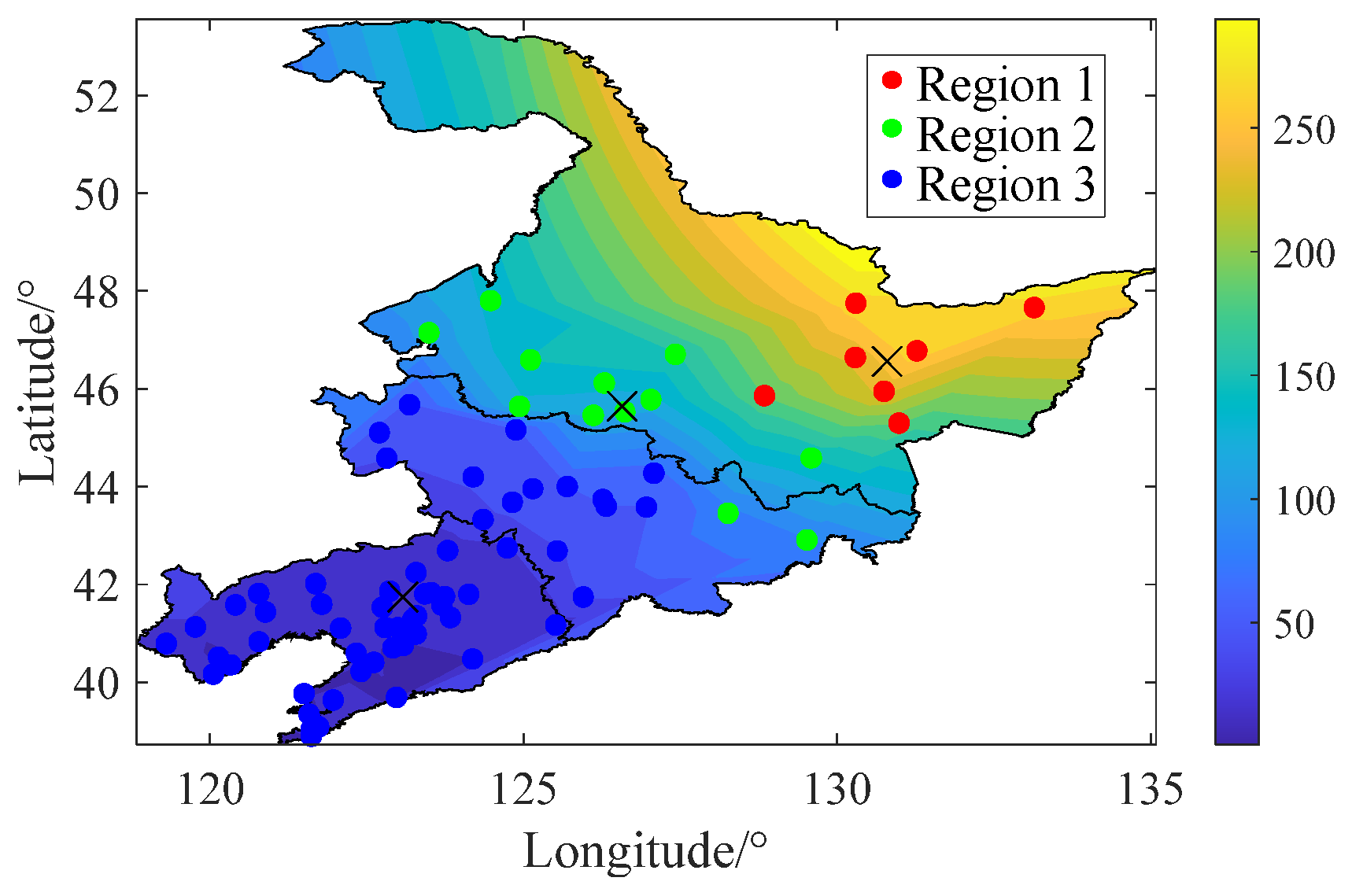
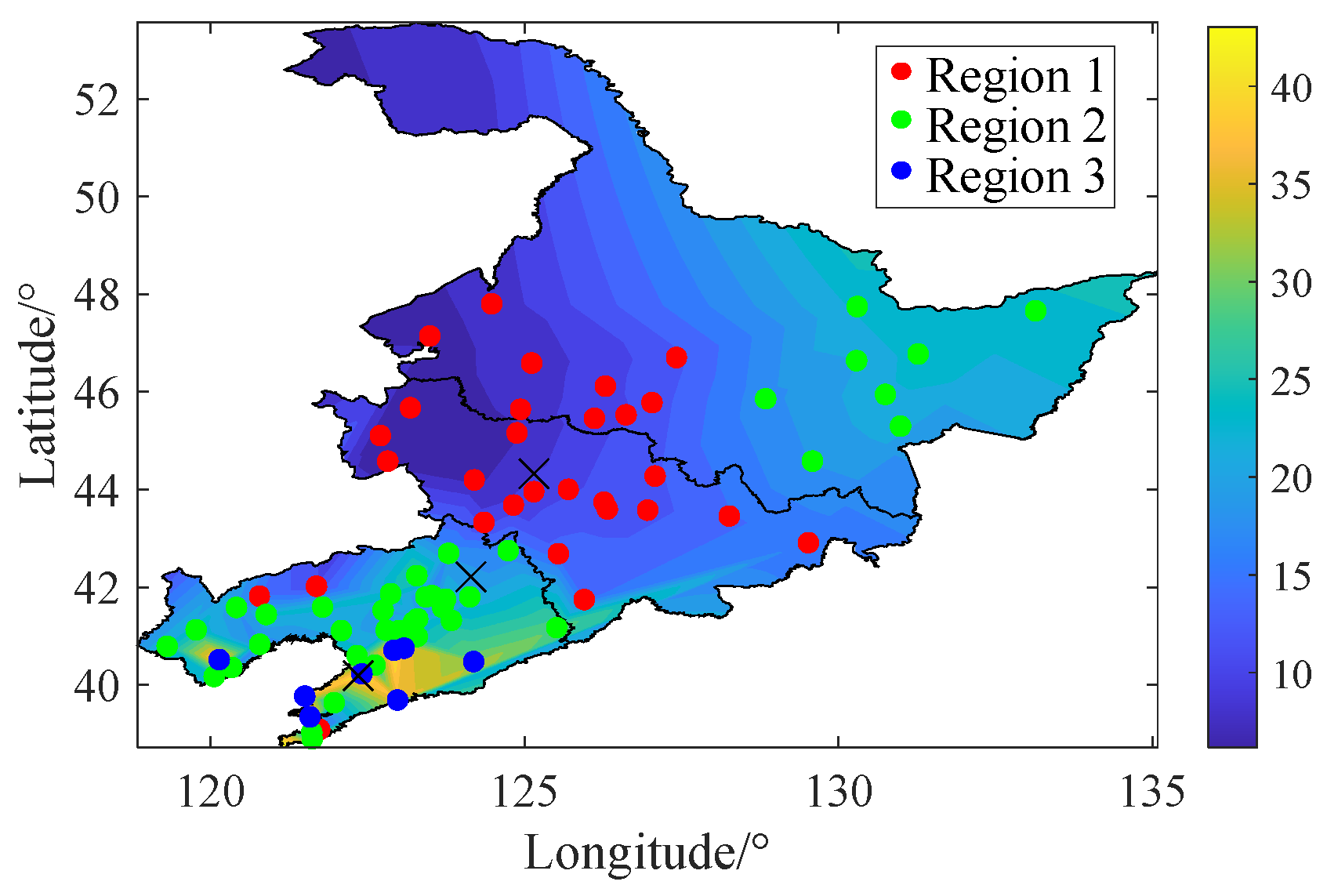
2.1. Quantitative Analysis of System Frequency Spatial Distribution Characteristics Based on Actual Grid Models

To mitigate the risk of frequency instability from large-scale integration of renewable energy, wind turbines employ a combination of virtual inertia and droop control, while PV systems and energy storage units utilize droop control to simulate the frequency response characteristics of synchronous machines. The differentiation in the distribution locations of frequency regulation resources and the diversification of control strategies have altered the network architecture and power flow distribution of the original power system. As demonstrated in [21], using a simple model, the frequency distribution of a system is highly sensitive to the parameters and distribution of frequency regulation resources. This paper further quantitatively analyzes the frequency distribution characteristics of each node in the actual grid model, selects equivalent indicators to measure the frequency dynamic response of local nodes, and characterizes the relationship between system power imbalance, inertia time constant, and rate of change of frequency (RoCoF) based on the rotor motion equation as shown in (1).

$${\displaystyle \frac{2H_{\mathrm{sys}}}{f_{\mathrm{N}}}}{\displaystyle \frac{\mathrm{d}f}{\mathrm{d}t}}=\Delta P_{\mathrm{sys}}-D\Delta f_{\mathrm{sys}}$$

(1)

where $\Delta P_{\mathrm{sys}}$ is the system power imbalance; $\Delta f_{\mathrm{sys}}$ is the system frequency deviation; $H_{\mathrm{sys}}$ is the equivalent inertia time constant; $D$ is the damping coefficient; $f_{\mathrm{N}}$ is the rated frequency of the system; and t is the time.

The nodal inertia can be defined in the case of neglecting the damping coefficient as follows:

$$H_j={\displaystyle \frac{\Delta P_j}{2F_j}}$$

(2)

$$F_j={\displaystyle \frac{1}{f_{\mathrm{N}}}}{\displaystyle \frac{\mathrm{d}{f}_j}{\mathrm{d}t}}$$

(3)

where $H_j$ is the equivalent inertia time constant of node j; $\Delta P_j$ is the power disturbance at node j; $f_j$ is the frequency of node j; $F_j$ is the rate of change of frequency of node j; and n is the number of nodes.

The regional center frequency $f_{\mathrm{COI}}$ can be obtained based on the frequency and equivalent inertia of each node of the system:

$$f_{\mathrm{COI}}={\displaystyle \frac{{\displaystyle \sum _{j=1}^n{H}_j{f}_j}}{{\displaystyle \sum _{j=1}^n{H}_j}}}$$

(4)

The average deviation value of each node from the center frequency is defined as the frequency dispersion S, as shown in (5). This parameter characterizes the degree of dispersion in the frequency response distribution across system nodes.

$$S={\displaystyle {\sum }_{j=1}^n\frac{{\displaystyle {\sum }_{t=i}^T{(f_j(t)-f_{\mathrm{COI}}(t))}^2}}{nT\Delta P_{\mathrm{sys}}}}$$

(5)

where $T$ is the total duration.

To analyze the impact of renewable energy integration and frequency regulation (FR) control on the frequency dynamic response of each node, an actual grid model was constructed on the PSASP software (v7.81.06) platform with renewable energy proportions set at 20% and 40%, respectively. The frequency response curves of multiple system nodes and COI nodes were compared under different scenarios, as shown in Figure 1 and Figure 2.

As shown in the results above, when the share of renewable energy increases from 20% to 40%, the system’s frequency nadir decreases, and the frequency dispersion increases. When new renewable energy is involved in frequency regulation, the system’s frequency support capability is significantly improved. However, the dispersion of system frequency also increases—by 7% for a 20% renewable energy share and by 13% for a 40% share. Overall, as the share of renewable energy increases, the spatial distribution of system frequency becomes more pronounced.

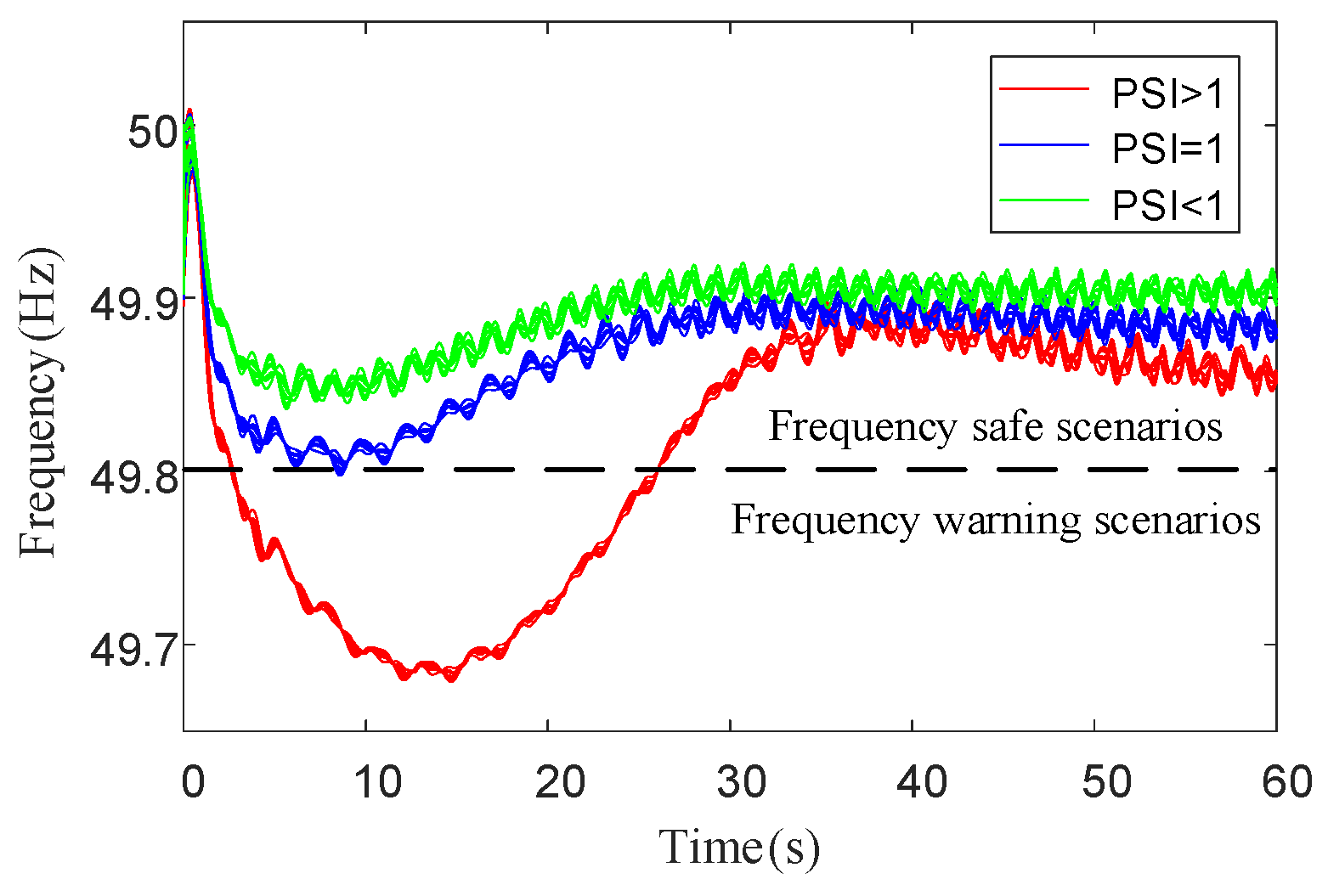
2.2. Frequency Security Posture Assessment Method

The power supply–demand imbalance in the power system is a fundamental cause of frequency shifts, and the magnitude of these shifts increases with the size of the power disturbance. After a disturbance occurs, the power imbalance is distributed among the generators according to the synchronized power coefficients, as shown in Equations (6) and (7).

$$\Delta P_{\mathrm{d}i}={\displaystyle \frac{P_{\mathrm{s}ik}}{{\displaystyle {\sum }_{j=1}^G{P}_{\mathrm{s}jk}}}}\Delta P_{\mathrm{L}}$$

(6)

$$P_{\mathrm{s}ik}=U_i{U}_k(B_{ik}\cos {\delta }_{ik0}-G_{ik}\sin {\delta }_{ik0})$$

(7)

where $P_{\mathrm{s}ik}$ is the synchronized power coefficient; $\Delta P_{\mathrm{L}}$ is the power disturbances; $\Delta P_{\mathrm{d}i}$ is the unbalanced power distribution among the generators; $G$ is the total number of the generators; $U_i$ and $U_k$ are the voltage of bus i and bus k, respectively; ${\delta }_{ik0}$ is the phase angle difference between bus i and bus k; and $B_{ik}$ and $G_{ik}$ are the real and imaginary parts of the derivative.

It can be seen that the smaller the electrical distance from the disturbance point, the larger the power imbalance amount borne by the generator set. The frequency response characteristics of each system node exhibit distributional differences, making it increasingly difficult for the traditional COI node frequency to accurately describe the system’s overall frequency response. Although node frequencies exhibit spatial heterogeneity after a disturbance, the node frequencies within a local area tend to have similar dynamic response processes, indicating a certain degree of spatial aggregation. Therefore, the frequency security posture assessment method is divided into two parts: observation node selection and frequency posture scenario discrimination.

The selection of observation points utilizes the equivalent inertia of system nodes as the clustering index, and the K-means clustering method is employed to group regions with similar frequency dynamic responses, helping to identify areas with weak frequency support capacity. Using the regional center frequency as a reference, the node with the highest correlation to the center frequency is identified as the regional characteristic node. This node represents the frequency dynamic process within the region and serves as an observation point for assessing the frequency security posture, as well as for the subsequent evaluation of the system’s frequency support capability, as shown in (8).

$$\rho ={\displaystyle \frac{\mathrm{cov}(f_i,f_{\mathrm{COI}})}{{\sigma }_{f_i}{\sigma }_{f_{\mathrm{COI}}}}}$$

(8)

where $\rho$ is the correlation coefficient between the frequency of node i ($f_i$) and the frequency of the regional center ($f_{\mathrm{COI}}$); $\mathrm{cov}(f_i,f_{\mathrm{COI}})$ is the covariance between $f_i$ and $f_{\mathrm{COI}}$; and ${\sigma }_{f_i}$ and ${\sigma }_{f_{\mathrm{COI}}}$ are the standard deviations of the two frequencies.

The tolerable amount of power disturbance can indirectly reflect the current system frequency posture. Using the characteristic nodes of each region as observation points, and with the maximum deviation of system frequency jointly constrained by the system’s equivalent inertia and primary frequency regulation as the analysis index, the frequency safety boundary $\Delta P_{\mathrm{bd}}$ is defined as the minimum active power perturbation needed to achieve a maximum frequency deviation of ±0.2 Hz at any observation node, regardless of the typical disturbance scenario. The power safety index (PSI) is defined as a power safety warning indicator, calculated as the ratio of the current power disturbance in the system to the power safety boundary, as shown in (9).

$$PSI={\displaystyle \frac{\Delta P_{\mathrm{L}}}{\Delta P_{\mathrm{bd}}}}$$

(9)

The frequency posture scenario discrimination classifies the system into two categories—frequency security and frequency warning scenarios—based on the PSI value, as illustrated in Figure 3. Obtaining PSI indicators based on actual grid operation scenarios enables the assessment of system frequency security posture and provides theoretical support for the subsequent design of cooperative control and parameter optimization methods for frequency regulation resources.

3. The Integrated Frequency Regulation Method Based on System Frequency Security Posture

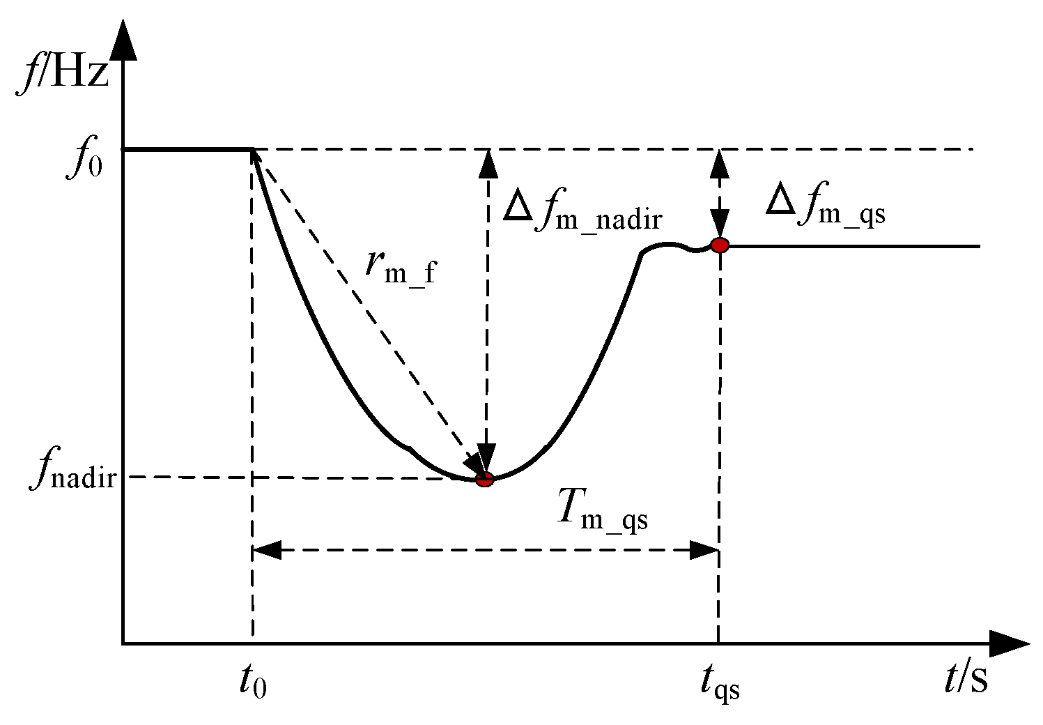
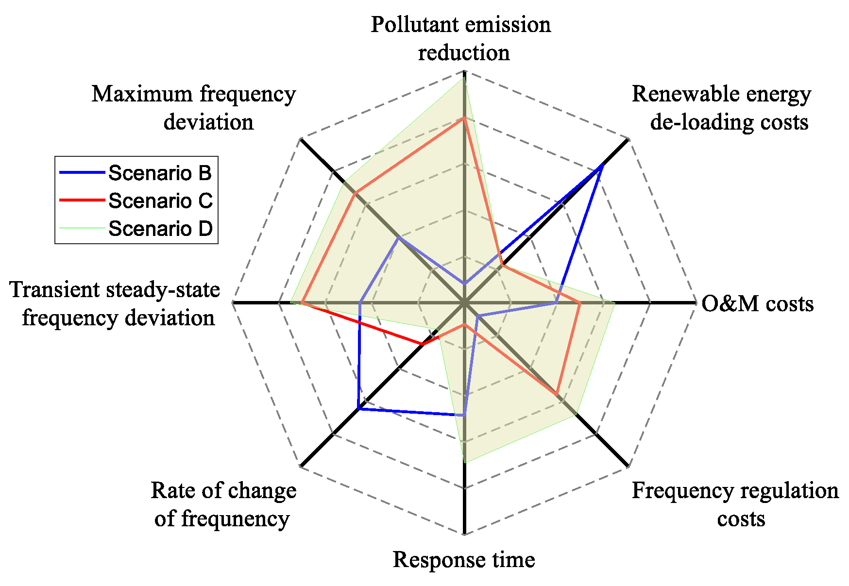
3.1. Comprehensive Evaluation Method for Frequency Regulation Effectiveness

The system frequency response characteristics reflect the system’s frequency support capability and are a key index for evaluating frequency regulation effectiveness. However, enhancing this capability is also associated with certain economic costs. Given the significant frequency spatial distribution characteristics of new-type power systems, the assessment of frequency regulation effects can no longer rely solely on the frequency of COI nodes in the system. The selection of measurement nodes for performance indicators is no longer limited to a single system node. Instead, it is based on the characteristics of the regional nodes to analyze the frequency response process both within the region and across the entire system. To comprehensively assess the overall frequency regulation effectiveness of the system, this paper establishes a multi-dimensional evaluation indicator system that accounts for diverse frequency regulation resources. The system evaluates multiple perspectives, including frequency regulation effect, economy, and environment, as shown in Figure 4. This evaluation process considers the economic costs associated with frequency regulation and pollutant emissions, as well as the frequency regulation performance of the system.

• Performance indicators

The key indicators of frequency response characteristics reflect the system’s frequency support capability. The performance indicators selected include maximum frequency deviation $\Delta f_{\mathrm{nadir}}$, transient steady-state frequency deviation $\Delta f_{\mathrm{qs}}$, change rate $r_{\mathrm{f}}$, and steady-state time $T_{\mathrm{qs}}$. To better address the spatial distribution characteristics among regions, the indicator data from the characteristic nodes of each region are considered comprehensively. Performance indicators for the response system are then derived based on the capacity weighting of each region.

$$X=[\Delta f_{\mathrm{nadir}},r_{\mathrm{f}},\Delta f_{\mathrm{qs}},T_{\mathrm{qs}}]$$

(10)

$$X_{ty}={\displaystyle \frac{{\displaystyle {\sum }_{m=1}^M{X}_{m\_ty}{S}_m}}{S}}$$

(11)

where X is the matrix of performance indicators; $X_{ty}$ is the value of a particular type of performance indicator in matrix X; $X_{m\_ty}$ is the value of a particular type of performance indicator for node m; M is the total number of measurement nodes; $S_m$ is the capacity of the measurement node m; and S is the total system capacity.

Taking the typical frequency response curve at node m of a region as an example, the specific method for obtaining the values of the performance indicators is shown in Figure 5. $\Delta f_{m\_\mathrm{nadir}}$ is the value of the deviation of the frequency nadir at measurement node m from the nominal frequency after the disturbance. $r_{m\_\mathrm{f}}$ is the rate of change of frequency during the period when the frequency at measurement node m falls to its lowest point after the disturbance. $\Delta f_{m\_\mathrm{qs}}$ is the transient steady-state frequency deviation from the nominal frequency when the frequency at measurement node m stabilizes after the disturbance. $T_{m\_\mathrm{qs}}$ is the stabilization time required for measurement node m to reach a transient steady state after the disturbance.

2.

Economic indicators

The frequency regulation cost, O&M cost, and standby compensation cost are selected as indicators for the economic category, accounting for the additional losses incurred from adjusting the output power of each generator in response to changes in system frequency. The economic costs of each node are summed to derive an indicator that reflects the overall economic performance of the system.

$$C=[C_{\mathrm{FMC}},C_{\mathrm{OM}},C_{\mathrm{RE}}]$$

(12)

$$C_{ty}={\displaystyle {\sum }_{m=1}^M{C}_{m\_ty}}$$

(13)

where C is the matrix of economic indicators of the system; $C_{ty}$ is the value of a particular type of economic indicator in matrix C; and $C_{m\_ty}$ is the value of a particular type of economic indicator for node m.

Specifically, $C_{m\_\mathrm{FMC}}$ is the frequency regulation cost resulting from the adjustment of active output by each type of frequency regulation resource, as shown in (14).

$$C_{m\_\mathrm{FMC}}={\displaystyle {\sum }_{type}^{tot}{\displaystyle {\sum }_{i=1}^{N_{\mathit{type}}}{\displaystyle {\sum }_{t=1}^T{c}_{type\_\mathrm{fmc}}\Delta P_{type\_i}(t)\Delta t}}}$$

(14)

where type is the category of frequency regulation resources, including thermal power units TH, renewable energy units RE, and energy storage power plants ST; tot is the total number of frequency regulation resource types; $N_{type}$ is the total number of similar frequency regulation resources; $c_{type\_\mathrm{fmc}}$ is the primary frequency regulation unit compensation cost for a particular type of frequency regulation resource; $\Delta P_{type\_i}(t)$ is the active power adjustment of unit i of a particular type of frequency regulation resource in Δt; and T and $\Delta t$ are the number of frequency regulation periods and the duration of frequency regulation, respectively.

$C_{m\_\mathrm{OM}}$ is the O&M cost incurred by each type of frequency regulation resource during the frequency regulation, as shown in (15).

$$C_{m\_\mathrm{OM}}={\displaystyle {\sum }_{type}^{tot}{\displaystyle {\sum }_{i=1}^{N_{\mathit{type}}}{\displaystyle {\sum }_{t=1}^T{c}_{type\_\mathrm{om}}{P}_{type\_i}(t)}\Delta t}}$$

(15)

where $c_{type\_\mathrm{om}}$ is the O&M cost per unit of electricity for a particular type of frequency regulation resource; $P_{type\_i}(t)$ is the active power of a particular type of frequency regulation resource unit i in $\Delta t$.

$C_{m\_\mathrm{RE}}$ is the cost incurred by the renewable energy power plant due to the de-loading operation as shown in Equation (16).

$$C_{m\_\mathrm{RE}}={\displaystyle {\sum }_{i=1}^{N_{\mathrm{RE}}}{\displaystyle {\sum }_{t=1}^T{c}_{\mathrm{re}}}}[P_{\mathrm{RE}\_i}^{\mathrm{pre}}(t)-P_{\mathrm{RE}\_i}(t)]\Delta t$$

(16)

where $N_{\mathrm{RE}}$ is the number of new renewable energy power plants; $P_{\mathrm{RE}\_i}(t)$ and $P_{\mathrm{RE}\_i}^{\mathrm{pre}}(t)$ are the actual active power output and the predicted maximum output of renewable energy plant i after de-loading during $\Delta t$, respectively; and $c_{\mathrm{re}}$ is the penalty cost per unit of wind and solar energy forgone.

3.

Environmental indicators

Given that frequency regulation in thermal power units leads to additional coal consumption and consequently increases environmental pollutants, pollutant emissions are selected as the evaluation indicator for the environmental category. The overall environmental indicator $A_{\mathrm{tp}}$ for the system is then obtained by summing the pollutant emission reduction across all regions.

$$A_{\mathrm{tp}}={\displaystyle {\sum }_{m=1}^M{A}_m}$$

(17)

where $A_m$ is the emission reduction of pollutants from thermal power units in region m due to frequency regulation.

$$A_m=(a\Delta P_{\mathrm{th}}^2(t)+b\Delta P_{\mathrm{th}}(t)+c)\Delta t$$

(18)

where a, b, c are the coefficients of the pollutant emissions as a function of power; $\Delta P_{\mathrm{th}}(t)$ is the power adjustment of the thermal power unit during the frequency regulation.

To evaluate the comprehensive effectiveness of the frequency regulation scheme, a combined weighting and TOPSIS assessment method is employed, integrating the entropy weighting method (EWM) and the analytic hierarchy process (AHP). Then, positive and intensive processing is conducted based on the types of indicators, leading to the determination of an assessment indicator that reflects the comprehensive effectiveness of the frequency regulation scheme. This provides a rigorous theoretical foundation and data support for the subsequent optimization of frequency regulation strategies.

Considering that the AHP is influenced by subjective weighting factors, the subjective weighting matrix ${\mathit{\omega }}^{\mathrm{AHP}}$ can be linked to the frequency security posture. Based on actual disturbance scenarios and the dispatch department’s priorities, two sets of subjective weight matrices—one prioritizing performance and the other, economy—are preset. The subjective weight matrix most suitable for the current scenario is then determined using the PSI metrics, as shown in (19). When PSI ≤ 1, economy is prioritized in the parameter optimization process, while performance is prioritized for PSI > 1.

$${\mathit{\omega }}^{\mathrm{AHP}}=\{\begin{array}{l}{\mathit{\omega }}_{eco}^{\mathrm{AHP}},PSI\le 1\\ {\mathit{\omega }}_{tec}^{\mathrm{AHP}},PSI>1\end{array}$$

(19)

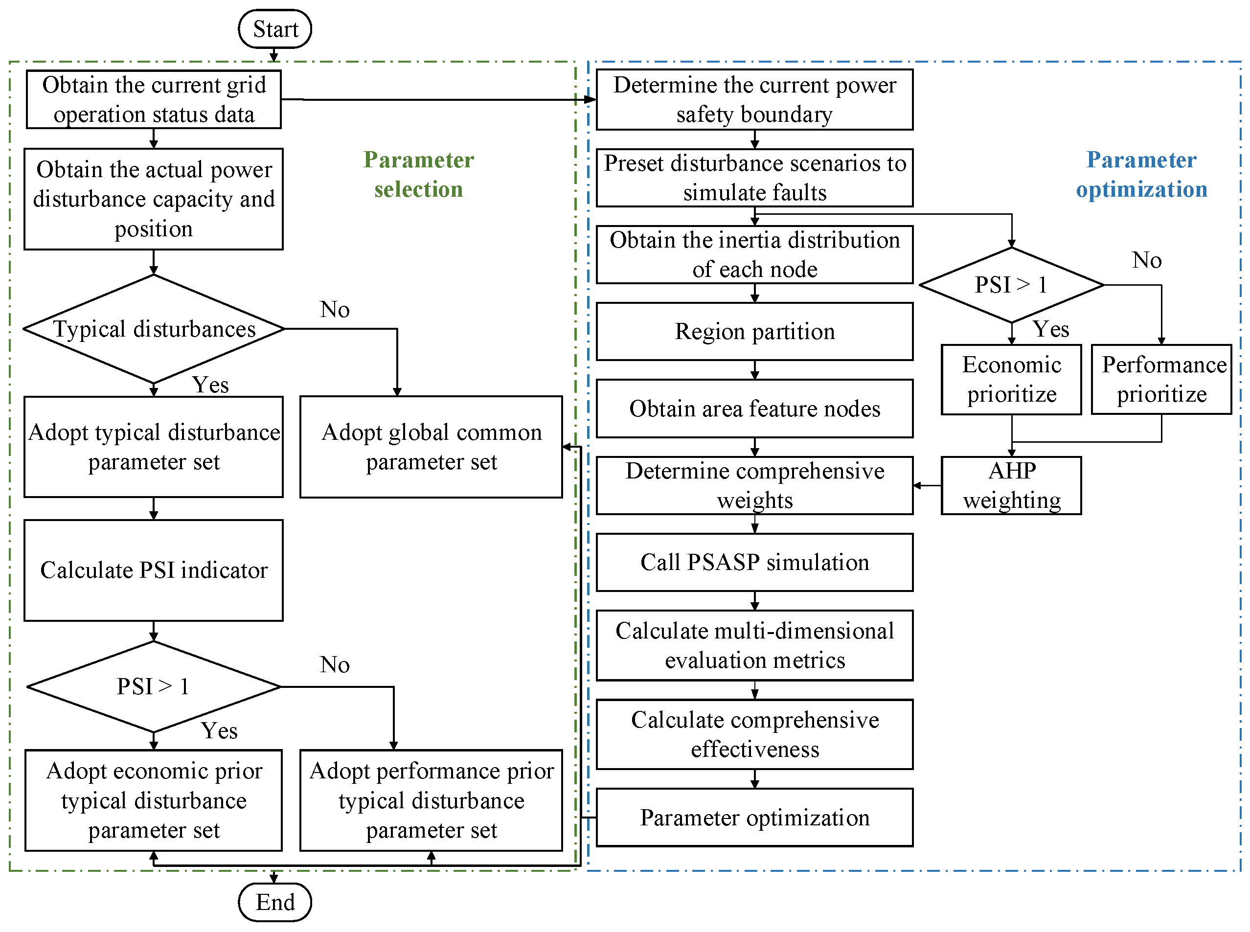
3.2. Parameter Optimization Method for Diversified Frequency Regulation Resources

In this section, the differential evolution algorithm is applied to optimize the virtual inertia coefficients, frequency regulation dead zones, regulation rates, de-loading coefficients, and other frequency regulation parameters for new-type resources such as wind, PV, and energy storage systems, utilizing the comprehensive effectiveness evaluation method proposed earlier. The optimization range for each parameter is determined according to the national standard GB/T40595-2021 [22].

The differential evolution algorithm consists of four main steps: mutation, crossover, boundary condition processing, and selection, as outlined in (20)–(25). The process begins with a vector population that is randomly perturbed. Subsequently, the parameter vectors that yield better performance are evaluated and used to replace those from the previous iteration.

• Mutation: First, mutated new individuals are obtained based on adaptive mutation factors by evaluating the better individuals from the original population:

  $$V_i^{g+1}=X_{r1}^g+F(X_{r2}^g-X_{r3}^g)$$

  (20)

  $$\{\begin{array}{l}F=2^{\lambda }{F}_0\\ \lambda =e^{1-{\displaystyle \frac{G_{\mathrm{m}}}{G_{\mathrm{m}}+1-g}}}\end{array}$$

  (21)

  where $V_i^{g+1}$ represents the value of the ith individual variant at the g + 1st iteration; $X_{r1}^g$, $X_{r2}^g$ and $X_{r3}^g$ are the values of the r 1st, r 2nd, and r 3rd individuals in the population at the gth iteration, respectively; r₁, r₂, and r₃ are integers randomly chosen to be mutually exclusive with i at NP population size; F is the variational operator, which serves to equalize the local and global searches; F₀ is the initial variation operator; and G_m is the total number of iterations.
• Crossover: This step involves simulating a genetic algorithm to construct a preparatory population by combining the original population with mutated individuals based on random probabilities.

  $$u_{ij}^{g+1}=\{\begin{array}{l}{v}_{ij}^{g+1},\mathrm{if}\mathrm{rand}(j)\le CR\\ x_{ij}^g,\mathrm{otherwise}\end{array}$$

  (22)

  $$U_i^{g+1}=[u_{i1}^{g+1},\cdots ,u_{ii}^{g+1},\cdots u_{in}^{g+1}]$$

  (23)

  where $u_{ij}^{g+1}$ and $v_{ij}^{g+1}$ are the parameter values of the jth term in the ith individual subjected to crossover and mutation at the g + 1st iteration, respectively; CR is a cross-operator; n is the total number of parameters; and $U_i^{g+1}$ is the preparatory population for g + 1st iterations.
• Boundary condition processing: Individual data are adjusted for new populations based on parameter group ranges:

  $$u_{ij}^{g+1}=\{\begin{array}{l}{u}_{\max j}^{g+1},if{u}_{ij}^{g+1}>u_{\max j}^{g+1}\\ u_{\min j}^{g+1},if{u}_{ij}^{g+1}<u_{\min j}^{g+1}\\ u_{ij}^{g+1},\mathrm{otherwise}\end{array}$$

  (24)

  where $u_{\max j}^{g+1}$ and $u_{\min j}^{g+1}$ are the maximum and minimum value of the jth parameter range; $u_{ij}^{g+1}$ is the value of the preparatory population for the jth parameter in the ith individual of the g + 1st iteration.
• Selection: Based on the assessment results of the original and preparatory populations, a new population is constructed based on merit:

  $$X_i^{g+1}=\{\begin{array}{l}{U}_i^{g+1},\mathrm{if}F(U_i^{g+1})>F(X_i^g)\\ X_i^g,\mathrm{otherwise}\end{array}$$

  (25)

  where $X_i^{g+1}$ is the final parameter value obtained in the g + 1st iteration; $F(U_i^{g+1})$ and $F(X_i^g)$ represents the assessment results when $U_i^{g+1}$ and $X_i^g$ are used as a selection variable, respectively.

The parameter optimization method for the control parameters such as virtual inertia coefficients, frequency regulation dead zones, droop coefficients, de-loading coefficients, etc., is implemented based on the comprehensive evaluation method of frequency regulation effectiveness and the differential evolutionary algorithm. Under the global power disturbance scenario and the preset typical disturbance scenario, the control parameters are iteratively updated based on the frequency regulation effectiveness evaluation results. This process determines the optimal parameter sets for each region, resulting in two types of optimal parameter sets: global common parameters and parameters specific to typical disturbance scenarios, as illustrated in Figure 6.

To ensure sufficient active power up-regulation space, the de-loading control of the renewable energy unit must be completed before the disturbance occurs. Therefore, in the typical disturbance scenario parameter set, the de-loading coefficients are pre-determined by the global common parameter set, while the remaining parameters are optimally adjusted based on the specific disturbance scenario to achieve efficient coordination of system frequency regulation resources. The global common parameter set is versatile and can be adapted to various power disturbance scenarios, effectively addressing the impact of disturbance locations on different node frequencies. The typical disturbance parameter set can fine-tune system area divisions and parameters based on typical disturbances identified from historical grid operation data, making it more adaptable to specific scenarios than the global general parameter set. The system flexibly selects between two parameter sets based on the operating conditions to achieve the optimal control solution for the current scenario.

3.3. Integrated Frequency Regulation Method for Diversified Resources

The integrated frequency regulation method proposed in this section assesses the frequency security posture using the system’s current operating state data and applies the parameter optimization approach from the previous section to generate two types of parameter sets tailored to the current operating state. The optimal parameter set is then chosen based on the actual disturbance encountered. This method consists of two main modules, parameter optimization and parameter selection, as illustrated in the flow chart in Figure 7.

The parameter optimization module is based on the current grid operation data and is pre-optimized to generate two types of alternative frequency regulation parameter sets. The specific optimization process can be divided into five steps: (1) The focus relationship between performance and economy in the frequency regulation objectives is adjusted based on the disturbance safety boundary and typical disturbance conditions, determining the AHP weight values for the subsequent process of frequency regulation effectiveness assessment. (2) The inertia distributions under different disturbance conditions are determined according to (1)–(3), followed by the division of similar measurement regions and the selection of regional characteristic nodes that best represent the frequency response properties of each region. (3) Based on the current frequency security posture, the subjective weight values are adjusted and combined with the objective weights to determine the comprehensive weights for the comprehensive evaluation of frequency regulation’s effectiveness. (4) The PSASP simulation results are analyzed based on regional characteristic nodes, the multi-dimensional evaluation index matrix is obtained, and the effectiveness of the current frequency regulation parameter scheme is determined using the TOPSIS evaluation methodology. (5) Using iterative differential evolutionary algorithms, the optimal set of frequency regulation parameters under typical disturbances is found, resulting in three types of frequency regulation parameter sets: globally generalized parameters, performance-prioritized typical disturbance parameters, and economy-prioritized typical disturbance parameters.

The parameter selection module identifies the optimal frequency regulation parameter set from the available alternatives based on the actual disturbance location and capacity and then finalizes the configuration of the frequency regulation parameters. After a disturbance occurs, the location and capacity of the actual disturbance are first estimated using monitoring equipment like PMUs, in conjunction with the disturbance capacity estimation method [23]. Then, if the disturbance occurs within a typical disturbance point or region, an economy- or performance-prioritized typical disturbance parameter set is further selected based on the frequency safety index (PSI). If the actual disturbance is atypical, a globally generalized parameter set with universal applicability is selected.

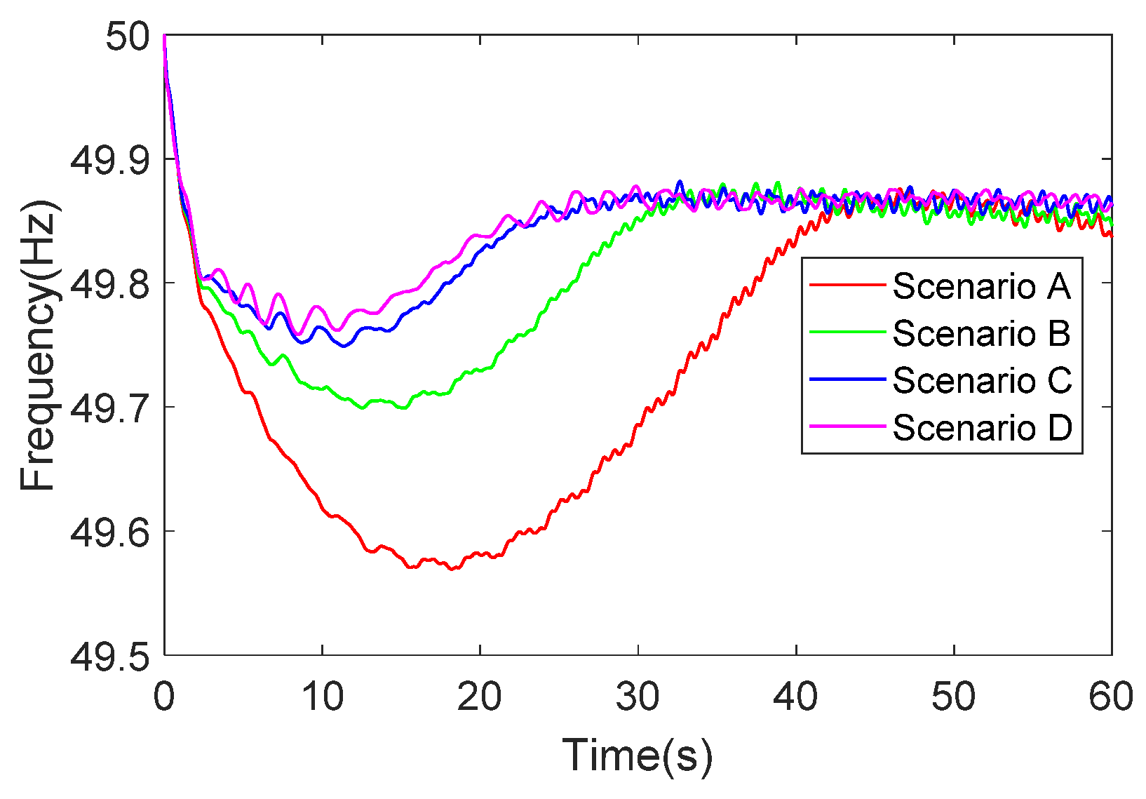
4. Simulation Verification

To verify the effectiveness and superiority of the integrated frequency regulation method based on the system frequency security posture proposed in this paper, a PSASP simulation model is constructed using operational data from an actual renewable energy feeder regional grid. The grid’s total active output is 53,400 MW, with contributions from thermal power (65%), hydropower (2%), nuclear power (11%), wind power (13%), and photovoltaic power (9%). The frequency safety boundary has been calculated to be 1600 MW. To verify the analysis in detail, two typical disturbance conditions are established based on whether the frequency safety boundary is crossed. The frequency regulation effects are then compared across three different frequency regulation schemes.

Scheme A: No system frequency regulation resources are involved except for conventional synchronous generators.

Scheme B: Renewable energy participates in system frequency regulation using a unified set of optimized frequency regulation parameters across all regions.

Scheme C: Renewable energy participates in system frequency regulation using the global common parameter set proposed in this paper, which is optimized separately for different regions.

Scheme D: Renewable energy participates in system frequency regulation using the integrated frequency regulation method based on the system frequency security posture, which is optimized separately for different regions and typical disturbances.

The population size is set to 10, with an initial variation factor of 0.8. The power safety boundary value is used as the disturbance capacity under the global disturbance scenario. The optimal parameter set for the current operation mode is obtained through steps including inertia partitioning, feature node selection, effectiveness evaluation, and differential evolutionary optimization. The system’s inertia distribution is depicted in Figure 8, and the globally optimized common parameters are detailed in

Table A1. Global common parameter set.

Region	Wind Power Units				Photovoltaic Units			Energy Storage System
	Dead Zone	Droop Coefficient	De-Loading Coefficient	Virtual Inertia Coefficient	Dead Zone	Droop Coefficient	De-Loading Coefficient	Dead Zone	Droop Coefficient
1	0.071	7.36	0.019	8.96	0.041	18.85	0.035	0.038	138
2	0.051	23.15	0.069	9.04	0.022	21.49	0.050	0.048	110
3	0.043	18.47	0.058	9.45	0.049	9.30	0.089	0.040	105

in Appendix A.

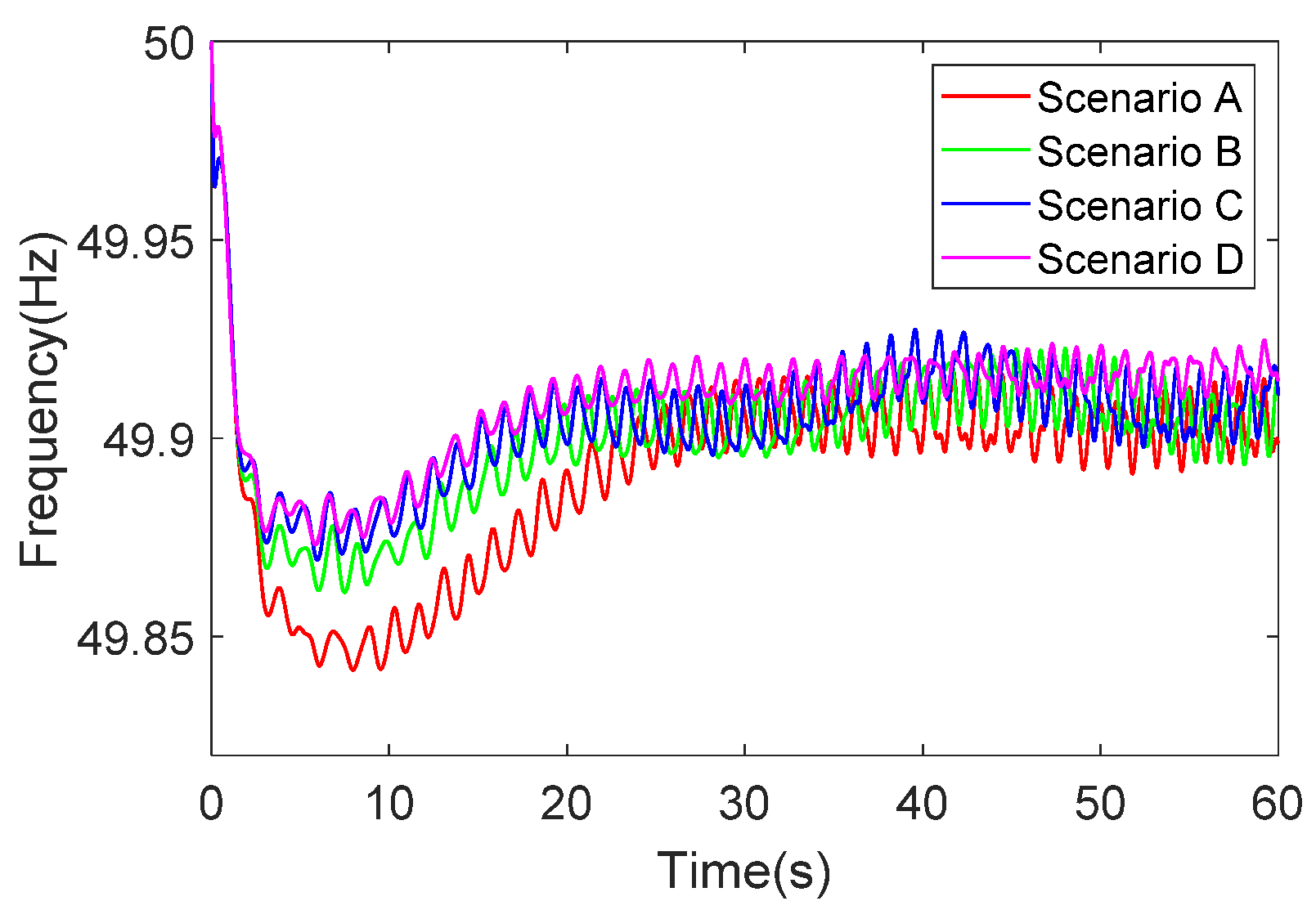
4.1. Typical Disturbance Condition I

Condition I simulates a fault-related cutover of a nuclear power unit, resulting in a system power deficit of 1120 MW, which does not breach the frequency safety boundary. The system’s inertia partitioning after the fault is illustrated in Figure 9. The frequency regulation parameters of scenario D are obtained according to the optimization algorithm as shown in

Table A2. Parameter set prioritized for the economics of typical disturbance condition I.

Region	Wind Power Units				Photovoltaic Units			Energy Storage System
	Dead Zone	Droop Coefficient	De-Loading Coefficient	Virtual Inertia Coefficient	Dead Zone	Droop Coefficient	De-Loading Coefficient	Dead Zone	Droop Coefficient
1	0.041	41.261	0.02	9.72	0.048	43.73	0.04	0.049	41
2	0.056	37.351	0.07	8.98	0.045	40.37	0.05	0.038	146
3	0.078	36.275	0.06	9.51	0.049	25.59	0.09	0.032	110

of Appendix A. The frequency response curves under each scheme are shown in Figure 10, and the frequency regulation performance and economic indicators are shown in

Table 1. Results of indicators under typical disturbance condition I.

Scenario	$\Delta {\mathit{f}}_{\mathbf{nadir}}$	$\Delta {\mathit{f}}_{\mathbf{qs}}$	${\mathit{r}}_{\mathbf{f}}$	${\mathit{T}}_{\mathbf{qs}}$	${\mathit{C}}_{\mathbf{FMC}}$	${\mathit{C}}_{\mathbf{OM}}$	${\mathit{C}}_{\mathbf{RE}}$	${\mathit{C}}_{\mathbf{ENV}}$
B	0.138	0.091	7.709	42.734	1.992	16.214	1.747	1.457
C	0.130	0.086	8.494	48.612	1.944	16.006	1.931	1.958
D	0.128	0.085	8.675	39.648	1.932	15.705	1.931	2.081

and Figure 11.

As shown in Figure 10, when compared to the scenario where new types of frequency regulation resources do not participate, Scenarios B, C, and D exhibit a significant reduction in overall frequency deviation and pollutant emission. In all cases, the frequency nadir is raised above 49.85 Hz. Moreover, the frequency regulation performance in scenarios C and D is better than in scenario B due to the optimization of parameters separately for different regions. As shown in Figure 11 and Table 1, since this disturbance does not exceed the frequency safety boundary, in Scenario D, which uses an economy-prioritized parameter set, the approach seeks to maintain performance indicators while reducing costs associated with frequency regulation (by 0.6%), operation and maintenance (by 1.9%), and mitigating pollutant emissions from coal combustion (by 6.3%) compared to Scenario C. This results in improved overall effectiveness in managing the typical disturbance and a reduction in system frequency dispersion.

4.2. Typical Disturbance Condition II

Condition II simulates a scenario where renewable energy is disconnected from the grid due to external factors such as line failures or adverse weather conditions, resulting in a system power deficit of 1900 MW, which breaches the frequency safety boundary. The system’s inertia partitioning after the fault is illustrated in Figure 12. The frequency regulation parameters of scenario D are obtained according to the optimization algorithm as shown in

Table A3. Parameter set prioritized for the performance of typical disturbance condition II.

Region	Wind Power Units				Photovoltaic Units			Energy Storage System
	Dead Zone	Droop Coefficient	De-Loading Coefficient	Virtual Inertia Coefficient	Dead Zone	Droop Coefficient	De-Loading Coefficient	Dead Zone	Droop Coefficient
1	0.069	10.35	0.02	9.76	0.026	49.89	0.04	0.040	149
2	0.038	18.35	0.07	9.42	0.054	24.88	0.05	0.039	145
3	0.061	24.03	0.06	9.09	0.028	41.60	0.09	0.038	83

of Appendix A. The frequency response curves under each scheme are shown in Figure 13, and the frequency regulation performance and economic indicators are shown in

Table 2. Results of indicators under typical disturbance condition II.

Scenario	$\Delta {\mathit{f}}_{\mathbf{nadir}}$	$\Delta {\mathit{f}}_{\mathbf{qs}}$	${\mathit{r}}_{\mathbf{f}}$	${\mathit{T}}_{\mathbf{qs}}$	${\mathit{C}}_{\mathbf{FMC}}$	${\mathit{C}}_{\mathbf{OM}}$	${\mathit{C}}_{\mathbf{RE}}$	${\mathit{C}}_{\mathbf{ENV}}$
B	0.302	0.146	3.305	36.391	3.528	28.612	0.968	0.334
C	0.252	0.138	5.835	29.646	3.543	29.065	1.931	0.708
D	0.240	0.136	4.609	28.690	3.691	29.775	1.931	1.128

and Figure 14.

As shown in Figure 13, Scenarios C and D significantly reduce the extent of frequency drop, minimize the maximum frequency deviation, and lower pollutant emissions compared to other scenarios. From Figure 14 and Table 2, it is evident that since this disturbance exceeds the frequency safety boundary, Scenario D, which employs performance-prioritized parameter set, enhances frequency regulation performance by increasing the participation of each unit, although this comes at the expense of reduced economic performance in frequency regulation. Compared to Scenario C, Scenario D shows significant improvements, including a 4.7% reduction in maximum frequency deviation, a 1.4% decrease in instantaneous steady-state frequency deviation, a 2% improvement in the frequency rate of change, and a 3.5% reduction in system frequency dispersion.

In summary, the results of the simulation and indicator calculation for Scheme C demonstrate that optimizing frequency regulation parameters based on system partitioning and spatial distribution characteristics can effectively enhance system frequency support capability while maintaining economic efficiency. The calculation results of Scenario D indicate that building upon Scenario C, further optimizing the parameters in advance for potential typical disturbance conditions and flexibly selecting parameter sets with different weights based on the frequency security posture after the disturbance occurs can better balance the grid’s needs for both frequency regulation performance and economic efficiency.

5. Conclusions

Addressing the growing challenges of spatial frequency distribution disparities and the ongoing decline in frequency support capacity in new-type power systems, this paper introduces an integrated frequency regulation method based on system frequency security posture. Building on the assessment method for system frequency security posture, the comprehensive evaluation method for frequency regulation effectiveness, and the differential evolution algorithm, the proposed approach optimizes the parameters of diversified frequency regulation resources by taking into account the spatial distribution characteristics of system frequency, grid operation scenarios, and actual disturbances. Simulation analysis based on an actual renewable energy feeder grid demonstrates that the method effectively adapts to varying grid frequency regulation performance and economic demands by flexibly adjusting the focus of parameter optimization under different operating conditions while also reducing system frequency dispersion. This offers effective technical support for the safe and economic operation of new-type power systems in the future. However, there are still potential areas for improvement, particularly regarding the reliability and stability of communication channels used for transmitting control parameters. These aspects warrant further exploration and optimization during the method’s promotion, application, and long-term operation.

References

1. Hamada, H.; Kusayanagi, Y.; Tatematsu, M.; Watanabe, M.; Kikusato, H. Challenges for a reduced inertia power system due to the large-scale integration of renewable energy. Glob. Energy Interconnect. 2022, 5, 266–273. [Google Scholar] [CrossRef]
2. Fang, J.; Li, H.; Tang, Y.; Blaabjerg, F. On the Inertia of Future More-Electronics Power Systems. IEEE J. Emerg. Sel. Top. Power Electron. 2019, 7, 2130–2146. [Google Scholar] [CrossRef]
3. Zhang, Z.; Zhang, N.; Du, E.; Kang, C.; Wang, Z. Review and Countermeasures on Frequency Security Issues of Power Systems with High Shares of Renewables and Power Electronics. Proc. Chin. Soc. Electr. Eng. 2022, 42, 1–24. [Google Scholar]
4. Shao, S.; Li, M.; Cai, H.; Liu, B.; Xu, X.; Guo, C. The Influence of Measured Trajectory Based Model Parameters Correcting on Simulation Precision of Power System Dynamic Frequency. Electr. Meas. Instrum. 2014, 51, 46–52. [Google Scholar]
5. Ma, N.; Xie, X.; Qin, X.; Su, L. Space-time Distribution Characteristics of Frequency in Power Systems with Renewable Energy Generators. In Proceedings of the 2021 IEEE 4th International Conference on Renewable Energy and Power Engineering (REPE), Virtual, 9–11 October 2021; pp. 227–232. [Google Scholar]
6. You, C.; Zhao, Y.; Hou, S.; Zhang, Y.; Lv, Y. Research on Centre of Inertia Based Frequency Sampling and System Frequency Distribution Characteristics. IEEE Access 2024, 12, 71371–71378. [Google Scholar] [CrossRef]
7. Zeng, F.; Zhang, J.; Zhou, Y.; Qu, S. Online Identification of Inertia Distribution in Normal Operating Power System. IEEE Trans. Power Syst. 2020, 35, 3301–3304. [Google Scholar] [CrossRef]
8. Dhara, P.K.; Rather, Z.H. A New Generator Clustering Approach for Power System Inertia Estimation with Reduced Number of Frequency Monitoring Nodes. In Proceedings of the 2021 IEEE Industry Applications Society Annual Meeting (IAS), 56th Annual Meeting of the IEEE-Industry-Applications-Society (IAS), Vancouver, BC, Canada, 10–14 October 2021. [Google Scholar]
9. Ekanayake, J.; Jenkins, N. Comparison of the response of doubly fed and fixed-speed induction generator wind turbines to changes in network frequency. IEEE Trans. Energy Convers. 2004, 19, 800–802. [Google Scholar] [CrossRef]
10. Shi, L.; Lao, W.; Wu, F.; Zheng, T.; Lee, K.Y. Frequency Regulation Control and Parameter Optimization of Doubly-Fed Induction Machine Pumped Storage Hydro Unit. IEEE Access 2022, 10, 102586–102598. [Google Scholar] [CrossRef]
11. Zeng, X.; Liu, T.; Wang, S.; Dong, Y.; Chen, Z. Comprehensive Coordinated Control Strategy of PMSG-Based Wind Turbine for Providing Frequency Regulation Services. IEEE Access 2019, 7, 63944–63953. [Google Scholar] [CrossRef]
12. Sun, M.; Min, Y.; Xiong, X.; Chen, L.; Zhao, L.; Feng, Y.; Wang, B. Practical Realization of Optimal Auxiliary Frequency Control Strategy of Wind Turbine Generator. J. Mod. Power Syst. Clean Energy 2022, 10, 617–626. [Google Scholar] [CrossRef]
13. Kheshti, M.; Ding, L.; Bao, W.; Yin, M.; Wu, Q.; Terzija, V. Toward Intelligent Inertial Frequency Participation of Wind Farms for the Grid Frequency Control. IEEE Trans. Ind. Inform. 2020, 16, 6772–6786. [Google Scholar] [CrossRef]
14. Tan, J.; Zhang, Y. Coordinated Control Strategy of a Battery Energy Storage System to Support a Wind Power Plant Providing Multi-Timescale Frequency Ancillary Services. In Proceedings of the 2018 IEEE Power & Energy Society General Meeting (PESGM), IEEE-Power-and-Energy-Society General Meeting (PESGM), Portland, OR, USA, 5–10 August 2018. [Google Scholar]
15. Li, D.; Chen, Z.; Xu, B.; Li, P.; Chen, H. Mechanism analysis and optimal dead zone parameter of wind-storage combined frequency regulation considering primary frequency regulation dead zone. Power Syst. Prot. Control 2024, 52, 38–47. [Google Scholar]
16. Liang, C.; Wang, P.; Han, X.; Qin, W.; Billinton, R.; Li, W. Operational Reliability and Economics of Power Systems with Considering Frequency Control Processes. IEEE Trans. Power Syst. 2017, 32, 2570–2580. [Google Scholar] [CrossRef]
17. Li, J.; Guo, Z.; Ma, S.; Zhang, G.; Wang, H. Overview of the “Source-grid-load-storage” Architecture and Evaluation System Under the New Power System. High Volt. Eng. 2022, 48, 4330–4341. [Google Scholar]
18. Xue, J.; Wang, D.; Tao, Y.; Qi, J.; Liao, S.; Mao, B.; Yao, L. Evaluation of Frequency Regulation Performance of Energy Storage Power Plants Based on Correlation Analysis and Combined Weighting Method. In Proceedings of the 2020 IEEE 4th Conference on Energy Internet and Energy System Integration (EI2), Wuhan, China, 30 October–1 November 2020; pp. 349–354. [Google Scholar]
19. Zhao, Y.; Xie, K.; Shao, C.; Lin, C.; Shahidehpour, M.; Tai, H.; Hu, B.; Du, X. Integrated Assessment of the Reliability and Frequency Deviation Risks in Power Systems Considering the Frequency Regulation of DFIG-Based Wind Turbines. IEEE Trans. Sustain. Energy 2023, 14, 2308–2326. [Google Scholar] [CrossRef]
20. Qiang, G.; Bing, S.; Congnan, G.; Jiajie, L.; Hao, C.; Yanbing, J.; Zihui, W. Evaluation of the Performance of Energy Storage System Participating in Grid Frequency Regulation. In Proceedings of the 2021 IEEE 5th Conference on Energy Internet and Energy System Integration (EI2), Taiyuan, China, 22–24 October 2021; pp. 4205–4209. [Google Scholar]
21. Li, J.; Lu, J.; Qian, M.; Tang, B.; Chen, N.; Peng, P. Research on System Partition Method of High Proportion Renewable Energy Power System Considering Dynamic Frequency Spatiotemporal Characteristics. In Proceedings of the 2023 4th International Conference on Advanced Electrical and Energy Systems (AEES), Shanghai, China, 1–3 December 2023; pp. 750–755. [Google Scholar]
22. GB/T40595-2021; Guide for Technology and Test on Primary Frequency Control of Grid-Connected Power Resource. China Electricity Council: Beijing, China, 2021.
23. Terzija, V.V. Adaptive underfrequency load shedding based on the magnitude of the disturbance estimation. IEEE Trans. Power Syst. 2006, 21, 1260–1266. [Google Scholar] [CrossRef]
Figure 1. Frequency response characteristics in different scenarios.
Energies 17 04886 g001
Figure 2. Frequency dispersions in different scenarios.
Energies 17 04886 g002
Figure 3. Frequency security posture partitioning.
Energies 17 04886 g003
Figure 4. Multi-dimensional evaluation indicator system.
Energies 17 04886 g004
Figure 5. Diagram of the method for obtaining performance indicators.
Energies 17 04886 g005
Figure 6. Predefined classification of disturbance scenarios.
Energies 17 04886 g006
Figure 7. Flow chart of the integrated frequency regulation method for diversified resources.
Energies 17 04886 g007
Figure 8. Equivalent inertia distribution under global disturbance.
Energies 17 04886 g008
Figure 9. Equivalent inertia distribution under typical disturbance condition I.
Energies 17 04886 g009
Figure 10. Frequency curves for different scenarios under typical disturbance condition I.
Energies 17 04886 g010
Figure 11. Radar chart of multi-dimensional evaluation indicators under typical disturbance condition I.
Energies 17 04886 g011
Figure 12. Equivalent inertia distribution under typical disturbance condition II.
Energies 17 04886 g012
Figure 13. Frequency curves for different scenarios under typical disturbance condition II.
Energies 17 04886 g013
Figure 14. Radar chart of multi-dimensional evaluation indicators under typical disturbance condition II.
Energies 17 04886 g014