Transient Momentum Balance—A Method for Improving the Performance of Mean-Value Engine Plant Models

Abstract

Mean-value engine models (MVEMs) are frequently applied in system-level simulations of vehicle powertrains. In particular, MVEMs are a common choice in engine simulators, where real-time execution is mandatory. In the case of real-time applications with prescribed, fixed sampling times, the use of explicit integration schemes is almost mandatory. Thus the stability of MVEMs is one of the main limitations when it comes to optimizing their performance. It is limited either by the minimum size of the gas volume elements or by the maximum integration time step. An innovative approach that addresses both constraints arises from the fact that the mass flow through the transfer elements of the MVEM is not modelled considering the quasi-steady assumption, but instead the mass-flow is calculated using a single transient momentum balance (TMB) equation. The proposed approach closely resembles phenomena in the physical model, since it considers both the flow-field history and the inertial effects arising from the time variation of the mass flow. It is shown in this paper that a consideration of the TMB equation improves the stability and/or the computational speed of the MVEMs, whereas it also makes it possible to capture physical phenomena in a more physically plausible manner.

1. Introduction

The development of future powertrains is being driven by the steadily increasing demands for improved energy consumption, lower emissions and better performance. To comply with these objectives it is necessary to understand and optimize energy-conversion phenomena in either conventional or advanced powertrains while considering specific technological and regulative constraints. For this reason, system-level simulations are indispensable for the efficient exploration of the design space during the concept development phase and during the powertrain design phase. Moreover, efficient system-engineering simulation models are also applicable as plant models for ECU (electronic control unit) development off-line in the office and online in HiL environments during the late calibration and validation phase. To support these tasks, system-engineering simulation models have to feature very fast computational times, whereas in HiL environments it is mandatory to strictly fulfill the real-time constraints. This does not only mean that the average computational times are shorter than the physical time of the system, but it is also inevitable that each time step is finished within the given time frame [1]. To allow sufficient time for the exchange of the data, the CPU time of each time step should be less than approximately half of the time step [1].

Therefore, hybrid MVEM that combine physical based models of the engine gas path with surrogate approaches (i.e., Static Neural Networks (e.g., [2,3]) or Support (e.g., [4]) and Relevance Vector Machines (e.g., [5])) to model engine-block are often used in HiL tasks. This modeling approach provides besides information on engine speed and load signals also sensor values of additional parameters of the engine gas path, e.g., intake manifold pressure and/or air mass flow, pressure before exhaust aftertreatment devices, several temperatures in the engine gas path…, which are the required inputs of modern ECUs. In addition, this modeling depth also efficiently supports analyses of different engine gas path configurations and related control strategies; as for example analyses of different air management approaches (e.g., [6]).

In the MVEM the discontinuous operation of the cylinders is replaced by the continuous processes for mass, enthalpy and species transport through the cylinders and the production of power. MVEMs thus neglect the discrete cycles of the cylinders and assume that all the processes are spread over the entire engine cycle [7]. This transformation of the cylinder representation is generally achieved by the introduction of a surrogate engine-block model that replicates the cycle-averaged behaviour of the cylinders [8,9]. Due to the continuous-flow characteristic of the cylinders and due to the neglected spatial variation of the variables, lumped-parameter MVEMs are not capable of capturing wave propagation phenomena in engine manifolds, which might influence the engine’s performance, as reported in, e.g., [9,10]. To better match the engine’s performance simulated with MVEMs, it is common to introduce additional inputs that consider non-modelled, unsteady effects, which are used to predict more accurate mean flows [9,10].

MVEMs are generally based on a bond-graph approach, where the two main groups of components are identified, i.e., the storage and the transfer components [11,12,13,14]. In the models of the engine gas path, the storage components with finite inertia comprise the mass/energy inertia in the gas volumes and the thermal inertia of the walls. The state of the components with finite inertia is described by solving balance equations in the form of ordinary differential equations (ODEs). The fluxes of all the adjoined transfer components can be seen as source or sink terms in the balance equations. It is commonly assumed that the transfer components do not feature inertial effects [7,10,11,15,16]. The state variables of the adjoined storage components are used as the input variables to evaluate the fluxes through the transfer elements, either out of algebraic correlations, given input maps or surrogate models, or as presented in this paper by solving the TMB equation. The sum of all the fluxes over a transfer component is zero. In the presented simulation model, the transfer elements comprise flow restrictions, heat exchangers, air cleaners, turbines and compressors. It should be noted that in some simulation models, e.g., [17], the heat exchanger is treated as a storage element; however, its treatment as a transfer element (which is presented in the next sections) enables a more physically plausible representation of the interaction between the heat exchanger’s geometry and its mass- and heat transfer functionality. Within this modelling framework the correct capacity of the engine manifolds is preserved by distributing the heat exchanger volume to the down- and up-stream storage element.

Explicit methods are frequently used to integrate the system of ODEs that describes the complete vehicle system. This is based on the fact that it is possible to comply with the real-time constraints if explicit methods are applied along with the appropriate modelling depth and a suitable set-up of the model, i.e., the CPU time of each time step should be less than approximately half of the time step. This constraint might be violated for high data-exchange frequencies when implicit methods are applied, since a Jacobian evaluation might require too much CPU time during certain time steps [1].

The time step of the integration method is thus influenced by the data-exchange frequency and by the stability criteria of the system of ODEs. Generally, the stability criteria in the engine manifolds (storage elements or plenums in the MVEM) require the smallest time steps [18]. According to the results shown in this paper and according to the data published in the literature [17,18], the characteristic time constants of the manifolds are in the range of a few milliseconds, whereas for high-speed engines with small exhaust manifolds they can also be smaller. Therefore, the typical integration steps of explicit solvers that ensure stable results are in the range of 1 ms for a passenger-car engine and up to 5 ms or even more for certain commercial-vehicle engines, which is also in agreement with the data published in [15,17,19].

Stability issues in storage elements are most frequently observed when the pressure ratio across the transfer element approaches unity, i.e., the pressures in the connected storage elements are similar [17]. In the case of a gasoline engine this corresponds to large throttle openings. Additionally, it is also possible to observe stability issues for large pressure ratios across the transfer element if the mass/volume of the fluid exchanged within one integration step is of the same order of magnitude as the mass/volume of the fluid in the manifold. To ensure the stability of the model, the integration time steps must be decreased, which might potentially violate the real-time constraints. To reduce the stiffness of the ODE system, it is also possible to group storage elements into common larger storage elements; however, this might have adverse effects on the accuracy of the model [9]. An alternative approach is proposed in [17], where the control volumes featuring fast dynamics are removed and the flows in and out of those volumes are considered as an algebraic constraint. By doing this, the original ODE that describes the volume with a fast response is transformed into the DAE. Similarly, in [7] the authors report that only relevant storage elements should be included in the MVEM in order to avoid stiffness in the system, which requires experience and/or iterations when constructing the model. Following the idea presented in [9], both latter approaches can lead to a reduced accuracy of the model.

It is proven in the paper at hand that stability of the model can also be enhanced through application of a TMB equation in the transfer elements of the MVEM. In the publically available literature two approaches to considering the momentum equation coupled to the compressor model [20,21] and to the compressor/turbine model [22] are presented, however in both approaches momentum equation is not primarily applied to improve the stability of the model, although stability implications are addressed in [20]. In [20,21] the momentum equation is considered to evaluate the compressor’s mass flow, which is needed as an input for the compressor model that relies on the independent variables of mass flow and the turbocharger’s speed, and in [22] the momentum equation is considered to improve the acoustic predictions and the prediction performance under pulsed-flow conditions. In both references the momentum equation was thus applied to the elements where mechanical work is added to, or extracted from, the flow.

The originality of this paper arises from the application of a single TMB equation to those transfer elements where no mechanical work is added to, or extracted from, the flow with the aim to enhance stability of the MVEMs. These elements namely most critically influence the stability of the model as presented in the paper. Within the framework of MVEMs, the group of transfer elements where no mechanical work is added to, or extracted from, the flow comprises the orifice, i.e., restriction and throttle, the heat exchanger, i.e., intercooler, air cleaner and exhaust after-treatment devices, whereas the method can also be applied to other transfer elements. It is shown in the paper that the introduction of the TMB equation improves the stability of the MVEMs, while also enabling the capturing of physical phenomena in a more physically sound manner. The application area of this innovative approach is thus mainly oriented, but not limited, to mean-value models in engine simulators where real-time execution with a prescribed, fixed sampling time is required.

2. Governing Equations

2.1. Storage Elements with Constant Volume

In a MVEM, the balance equations of mass, energy and species concentrations, together with the equation of state, form a sufficient set of equations for the storage elements. The species balance equations are considered in the proposed model to reflect the influence of the gas composition on the physical properties of the fluid for the complete engine operating map, e.g., different EGR rates, different exhaust-gas temperatures and compositions. This is required to more correctly model the flow through the transfer elements and states in the storage elements.

The framework of equations was laid out in a general way, enabling the consideration of an arbitrary number of species, where:

$$\mathbf{W}={\left[w_1\dots w_N\right]}^T$$

(1)

In the present analysis, the species vector, W, represents the burned fuel (FB), the combustion products (CPs) and the fuel vapour (FV):

$$\mathbf{W}={\left[w_{FB},w_{CP},w_{FV}\right]}^T$$

(2)

where $w_{FB}$ gives the concentration of the fuel that was burned, i.e., converted from FV to FB, whereas $w_{CP}$ gives the concentration of the corresponding CPs, i.e., burned fuel and air that were used in the combustion. The species concentration of the air is derived using:

$$w_{air}=1-w_{CP}-w_{FV}$$

(3)

In the temperature and pressure ranges characteristic for engine manifolds it is sufficiently accurate to use the ideal gas law:

$$pV=m\frac{\Re }{M}T=mRT$$

(4)

due to relatively low pressures in the engine manifolds [23].

The mass-balance equation of the storage elements is:

$$\frac{\mathrm{d}m}{\mathrm{d}t}={\displaystyle \sum _j{\dot{m}}_j}$$

(5)

where time (t) is the independent variable and j runs over all the transfer elements (TE) attached to the storage elements.

The rate of change of species concentration comprises the species concentration variation due to mass transfer and the species concentration variation due to chemical reactions (CRs) if present. It follows that:

$$\frac{\mathrm{d}{w}_k}{\mathrm{d}t}=\frac{{\displaystyle \sum _j\left(w_{k,GE}-w_{k,SE}\right){\dot{m}}_j}}{m}+\frac{\mathrm{d}{w}_{k,CR}}{\mathrm{d}t}$$

(6)

where the index SE denotes the storage element and GE denotes:

$$GE=\{\begin{array}{c}SE\mathrm{for}{\dot{m}}_j\le 0\\ TE\mathrm{for}{\dot{m}}_j>0\end{array}$$

(7)

The first law of thermodynamics for an open system equals:

$$\frac{\mathrm{d}E}{\mathrm{d}t}=\frac{\mathrm{d}Q}{\mathrm{d}t}+\frac{\mathrm{d}H}{\mathrm{d}t}$$

(8)

where the term:

$$\frac{\mathrm{d}Q}{\mathrm{d}t}=\frac{\mathrm{d}{Q}_{HT}}{\mathrm{d}t}+\frac{\mathrm{d}{Q}_{CR}}{\mathrm{d}t}$$

(9)

covers heat transfer and chemical reactions, if present, and the term:

$$\frac{\mathrm{d}H}{\mathrm{d}t}={\displaystyle \sum _j{h}_{GE}{\dot{m}}_j}$$

(10)

covers the enthalpy flows through the attached transfer element. The index GE is defined by Equation (7).

In analogy with the derivation presented in Reference [24], it is possible to reformulate the first law of thermodynamics by considering the equations given in this section to be explicit in pressure:

$$\frac{\mathrm{d}p}{\mathrm{d}t}=\frac{C}{m}\left[\frac{\mathrm{d}Q}{\mathrm{d}t}+\frac{\mathrm{d}H}{\mathrm{d}t}-\left(e-\frac{\partial e}{\partial T}\frac{T}{A}\right)\frac{\mathrm{d}m}{\mathrm{d}t}-m{\displaystyle \sum _k\left(\frac{\partial e}{\partial w_k}-KT\frac{\partial R}{\partial w_k}\right)\frac{\mathrm{d}{w}_k}{\mathrm{d}t}}\right],$$

(11)

where:

$$A=1+\frac{\partial R}{\partial T}\frac{T}{R}$$

(12)

$$B=1-\frac{\partial R}{\partial p}\frac{p}{R}$$

(13)

$$C=\frac{1}{\frac{\partial e}{\partial p}+\frac{\partial e}{\partial T}\frac{T}{p}\frac{B}{A}}$$

(14)

and:

$$K=1+\frac{\partial e}{\partial T}\frac{1}{RA}$$

(15)

Frequently, the first law of thermodynamics is reformulated to be explicit in temperature; however, the approach proposed in Equation (11) ensures better stability of the model. This is due to the fact that the flows through the transfer elements are mainly influenced by the pressures in the up- and down-stream storage elements. The approach proposed in Equation (11) thus ensures immediate updates of the pressures in the storage elements as the system of ODEs is solved.

Equation (11) is evaluated considering dependencies of gas properties, i.e., internal energy (e), specific gas constant (R) and all partial derivatives of both properties, on temperature (T), pressure (p), and species concentrations ($w_{FB},w_{CP},w_{FV},w_{air}$). Gas property database can be prepared for arbitrary fuel or fuel blend taking into account chemical equilibrium considerations. In this way it is possible to determine accurate values of the gas property parameters with respect to the temperature, pressure and species concentrations, which are required to model the engine’s operation during various steady-state and transient operating conditions. The term $\partial e/\partial w_{FB}$ might not be negligible at rich air-fuel ratios and thus it needs to be considered when a higher fidelity of the results is required. Under these operating conditions the value of the specific gas constant and its derivative $\partial R/\partial w_k$ also changes due to the presence of molecules with small molecular masses. It is also meaningful to consider heat transfer ($\mathrm{d}{Q}_{HT}$) in Equation (11), since it represents a significant energy loss in the exhaust systems and thus it is crucial for the modelling of turbocharged engines and for modelling the thermal response of the exhaust system.

2.2. Transfer Elements without Inertia

In MVEMs the orifice equation is commonly used to model the transition from the total state in a storage element to the flow field in a transfer element. It is also common to consider compressible flow if a higher accuracy is demanded (see, e.g., references [7,25]). The orifice equation is given by:

$$\dot{m}=\mu A_{geom}{p}_{up}\sqrt{\frac{2}{R_{up}{T}_{up}}}\psi ,$$

(16)

where $\psi$ changes for subsonic or sonic flow conditions as:

$$\psi =\sqrt{\frac{\kappa }{\kappa -1}\left[{\left(\frac{p_{down}}{p_{up}}\right)}^{\frac{2}{\kappa }}-{\left(\frac{p_{down}}{p_{up}}\right)}^{\frac{\kappa +1}{\kappa }}\right]}$$

(17)

for subsonic flow and:

$$\psi ={\left(\frac{2}{\kappa +1}\right)}^{\frac{1}{\kappa -1}}\sqrt{\frac{\kappa }{\kappa +1}}$$

(18)

for sonic flow.

Similarly, the velocity in the orifice is given as:

$$u_{or}=\sqrt{2\cdot R\cdot T_{up}}\cdot v,$$

(19)

where v is given by:

$$v=\sqrt{\frac{\kappa }{\kappa -1}·\left(1-{\left(\frac{p_{down}}{p_{up}}\right)}^{\frac{\kappa -1}{\kappa }}\right)}$$

(20)

for subsonic flow and by:

$$v=\sqrt{\frac{\kappa }{\kappa +1}}$$

(21)

for sonic flow.

The enthalpy and species flows taken from the upstream storage element are calculated by multiplying the corresponding upstream values with the mass flow given by Equation (16).

Equation (16) is commonly used to model the flow through the restriction, throttles and related orifice-like elements. If these elements feature a variable flow cross-section, e.g., a throttle, not only $A_{geom}$ but also $\mu$ changes in the general case. To reduce the number of computational operations and model-preparation expenses, $A_{eff}=\mu A_{geom}$ is frequently introduced to account for both these two effects. Therefore, in the presented case, the value $A_{geom}$ is kept constant and only the value of the flow coefficient ($\mu$) is steered to control the $A_{eff}$ and the mass flow.

Equation (17) has an infinite gradient for $p_{down}=p_{up}$ [7], which might influence the stability of the equation system. To overcome this problem, a laminar flow condition can be assumed for very small pressure ratios, as reported in [7]. This approach relies on the assumption that there exists a threshold:

$${\mathrm{\Pi }}_{tr}=\frac{p_{down}}{p_{up}}{|}_{tr}<1$$

(22)

above which smooth approximation of the form:

$$\psi \left(\mathrm{\Pi }\right)=a\cdot {\left(\mathrm{\Pi }-1\right)}^3+b\cdot \left(\mathrm{\Pi }-1\right)$$

(23)

with:

$$a=\frac{{\psi }_{tr}^{\prime }\cdot \left({\mathrm{\Pi }}_{tr}-2\right)-{\psi }_{tr}}{2\cdot {\left({\mathrm{\Pi }}_{tr}-1\right)}^3},b={\psi }_{tr}^{\prime }-3\cdot a\cdot {\left({\mathrm{\Pi }}_{tr}-1\right)}^2$$

(24)

is valid. $\mathrm{\Pi }=p_{down}/p_{up}$ and ${\psi }_{tr}$ is the value of $\psi$ and ${\psi }_{tr}^{\prime }$ is the derivative of $\psi$ at the threshold ${\mathrm{\Pi }}_{tr}$. The form of equation (23) guarantees finite gradient at $\mathrm{\Pi }=1$, symmetric behavior around $\mathrm{\Pi }=1$ and smooth transition to Equation (17) at ${\mathrm{\Pi }}_{tr}$.

Although in some simple MVEMs the heat exchangers and exhaust after-treatment devices are modelled using Equation (16), it is generally not sufficiently accurate just to consider the pressure drop due to the inflow into the pipe [Equation (16)] and to neglect the frictional pressure drop associated with the flow through these elements. The frictional pressure drop can be captured by artificially increasing the downstream pressure in Equation (16), where pressure in the downstream storage element is increased for an estimate of the frictional pressure drop, or by artificially decreasing the flow coefficient. Another, more consistent, approach is to couple Equation (16) with the 1D, steady-state, pipe-flow equations. The latter approach is suitable for modelling the quasi-steady flow through heat exchangers and exhaust after-treatment devices. In this case, the equations for the flow through the orifice are coupled with mass, momentum and energy equations on the left-hand and right-hand sides of a pipe-like section, as shown in Figure 1. The mass, momentum and energy equations of a pipe-like section with the constant cross-section ($A_L=A_R=A$) are given by:

$${\dot{m}}_{or}={\dot{m}}_L={\dot{m}}_R$$

(25)

$$u_{\mathrm{L}}^2\cdot {\rho }_{\mathrm{L}}-u_{\mathrm{R}}^2\cdot {\rho }_{\mathrm{R}}-p_{\mathrm{R}}+p_{\mathrm{L}}=p_{\mathrm{F}\mathrm{r}}$$

(26)

$${\dot{H}}_{0,up}={\dot{H}}_{0,or}={\dot{H}}_{0,L}={\dot{H}}_{0,R}-{\dot{Q}}_{HT}$$

(27)

where L (left) and R (right) represent the up- and down-steam side of the pipe-like element, respectively. This approach also enables the modelling of the pressure recovery from the orifice to the left-hand side of the pipe. From Equation (27) the temperature in the orifice is calculated as:

$$T_{or}=T_{up}-\frac{{u^2}_{or}}{2\cdot c_{p,or}}$$

(28)

where $u_{or}$ is given by Equation (19). Computational procedure of the quasi-steady 1D flow equations is given in Section 2.4.

Figure 1. Scheme of the transfer element consisting of the orifice followed by the element of the length L, which in the case of the TMB represents the inertia of the flow field.

Figure 1. Scheme of the transfer element consisting of the orifice followed by the element of the length L, which in the case of the TMB represents the inertia of the flow field.

2.3. Transfer Elements with Inertia

Although some transfer elements, e.g., throttles, restrictions, air cleaners, are relatively short, others, e.g., heat exchangers and exhaust after-treatment devices, are generally much longer. By considering realistic pressure ratios it can be concluded that in most transfer elements the times needed to accelerate the flow to the velocities encountered in the engine manifolds are longer than the integration time steps of the MVEMs that are addressed above. Therefore, in such transfer elements, it is convenient, for preserving the consistency of the simulation model with the physical phenomena and for enhancing the stability of the simulation model, to consider the TMB.

Due to the fact that MVEMs do not consider the pressure pulsations caused by cyclic engine operation (since the engine is treated as a continuous flow device) the introduction of wave dynamics schemes, e.g., common 1D schemes [26] or the Quasi-Propagatory Model [27], would be superfluous. It is thus possible to represent any transfer element as a single 1D element (with the length L) where the inflow from the upstream element is modelled by Equation (16) and at the other end there is an outflow through the open end into the downstream storage element, as shown in Figure 1. In accordance with the modelling depth of the MVEMs it is assumed that the mass flow through the orifice equals the mass flow through the pipe, see Equation (25). In this way the integration time step of the proposed approach is not limited by the CFL criterion characteristic for the wave dynamic schemes [26,27] and can thus be larger. To ensure a high level of generality, it is possible that the inflow flow coefficient is smaller than unity, as sketched in Figure 1. In addition, to ensure the high robustness and general applicability of the model, the sonic outflow is also considered in the model.

The transient 1D momentum balance equation for a pipe is given by:

$$\frac{\partial \left(\rho \cdot u\cdot A\right)}{\partial t}=-\frac{\partial \left(\left[\rho \cdot u^2+p\right]\cdot A\right)}{\partial x}-\rho \cdot G\cdot A$$

(29)

For a single cell, Equation (29) is integrated in x, considering a staggered grid, i.e., the net efflux of momentum is exchanged through the boundaries of the cell and the pressure forces across the cell are also given at the end faces, whereas the mass-flow derivative corresponds to the middle of the cell, as depicted in Figure 1. Similarly, integrating the term $\rho \cdot G\cdot A$, which in Equation (29) accounts for the wall friction, over the complete cell length, gives the cell-pressure drop $p_{Fr}$. In the evaluation of the term $p_{Fr}$ it is possible to apply various correlations to evaluate the friction losses suitable for particular elements. This yields:

$$\frac{\mathrm{d}\dot{m}}{\mathrm{d}t}=A\cdot \left(\frac{{\left[\rho u^2\right]}_L-{\left[\rho u^2\right]}_R}{L}+\frac{p_L-p_R-p_{Fr}}{L}\right).$$

(30)

The innovative idea presented in this paper thus arises from the fact that the mass flow through the transfer element in the MV engine model is not calculated by Equation (16) (or its coupling with Equations (25)–(27) as introduced in Section 2.2) but instead the mass-flow derivative is calculated by Equation (30) and the mass flow through the element is obtained by integrating the mass-flow derivative. This approach more closely resembles reality, since it considers both the flow-field history and the inertial effects arising from the time variation of the mass flow, which indeed influences the flow at the observed time instant.

These facts are also crucial for improving stability of the simulation model when using large integration time steps. If the inertial effects arising from the time variation of the mass flow are not considered, i.e., assuming quasi-steady behaviour of the transfer elements, it is very likely that the system will exhibit instabilities in the form of the oscillating velocity in the transfer element for larger integration time steps, as also argued in [27]. Therefore, the approach proposed in this section has the potential to improve the stability of the simulation model.

As shown in Figure 1, the flow enters the cell through an orifice that is modelled as an isentropic and adiabatic device (i.e., total enthalpy is conserved):

$${\dot{H}}_{0,up}={\dot{H}}_{0,or}={\dot{H}}_{0,L}.$$

(31)

If the heat transfer takes place between the state L and R (Figure 1), Equation (27) is used to account for the variation in the total enthalpy. This approach enables the modelling of isobaric flow from the orifice to the state L in the pipe, i.e., p_or = p_L, or it is possible to introduce a pressure-recovery model for the flow from the orifice to the state L.

The configuration shown in Figure 1 is well suited to modelling heat exchangers and exhaust after-treatment devices, whereas its applicability to model throttles might be less intuitive, although the configuration with one orifice and an inertial element representing the inertial effects arising from the time variation of the mass flow quite realistically represent a real throttle device. The configuration shown in Figure 1 is also more suitable for modelling throttles than the configuration with the orifice in the middle of the pipe. The latter configuration would require the modelling of an inflow boundary followed by the pipe section, an orifice, the second pipe section and the outflow boundary, which would lead to different flow characteristics compared to those of Equation (16). In Equation (30) the flow acceleration from L to R influences the mass-flow derivative, which is mandatory for the high-fidelity modelling of heat exchangers. However, the term ${\left[\rho u^2\right]}_L-{\left[\rho u^2\right]}_R$ causes a deviation from the flow characteristics of Equation (16). To match the steady-state flow characteristics of Equation (16), while still considering the inertial effects arising from the time variation of the mass flow, it is possible to modify Equation (30) as:

$$\frac{\mathrm{d}\dot{m}}{\mathrm{d}t}=A\cdot \left(\frac{p_L-p_R}{L}\right).$$

(32)

Remark I: It is easily possible to combine the transfer elements with and without inertia in the same engine model. If it is intended to model the transfer element without the TMB the framework presented in Section 2.2 should be used. Tests on various engine models have shown that the stability of the model can already be improved if the TMB is only considered in some elements that are most prone to instabilities. The framework for analysing the stability of the system, which is introduced in Section 4 and Appendix A, might be used to decide on the use of the TMB.

Remark II: If the TMB is applied it is often possible to artificially prolong the elements without noticeably influencing the transient engine results within the framework of the MVEM, as shown in Section 5.4. In this way the stiffness of the model is reduced, i.e., the stability of the model (system) is enhanced by retaining the integration scheme and the time step, as analysed in Section 5 and Appendix A.

Remark III: The objective of this paper is to analyse the application of the TMB in the MVEMs used for engine simulators, where real-time execution and thus the application of explicit solvers is needed. Unlike the real-time simulations, various types of implicit integration schemes for ODEs can be applied in off-line simulations. Implicit schemes can allow for the application of very large time steps and they can also be well suited to resolving stiff systems. When implicit schemes are applied, a consideration of the TMB might be redundant as implicit solvers are well suited to resolving stiff systems and thus adding more states increases the computational burden.

2.4. Computational Procedure of 1D Equations

Transient 1D equations of the TMB model [Section 2.3—Equation (30) or (32) and related equations] and quasi-steady 1D equations [Section 2.2—Equation (26) and related equations] should be solved coupled with corresponding boundary conditions to model the flow through the transfer element.

The computational procedure of the transient 1D equations of the TMB model can be summarized as follows:

• Evaluation of orifice parameters: $p_{or}$, $u_{or}$ and $T_{or}$ are evaluated from the known value of $\dot{m}$ using the orifice equations given in Section 2.2, i.e., Equations (16), (19) and (28).
• Evaluation of parameters at state L: $p_L$ is determined using either the isobaric or pressure-recovery model for the flow from the orifice to the state L in the pipe. The temperature on the left-hand side of the pipe T_L is calculated by considering Equations (25) and (31), since the velocity and temperature for the state L are not known. By assuming $c_{p,L}=c_{p,or}$ and $R_L=R_{or}$, which is reasonable in the majority of the cases, the equation for T_L is derived as:

  $$T_L=\frac{-1+\sqrt{1+2\cdot {\mu }^2\cdot \frac{1}{{T^2}_{or}}\cdot \frac{{u^2}_{or}}{c_{p,or}}\cdot \left(T_{or}+\frac{{u^2}_{or}}{2\cdot c_{p,or}}\right)}}{{\mu }^2\cdot \frac{1}{{T^2}_{or}}\cdot \frac{{u^2}_{or}}{c_{p,or}}}$$

  (33)

  whereas it is also possible to iterate on $c_{p,L}$ and $R_L$. With known values of the temperature, pressure and specific gas constant the density ${\rho }_L$ is calculated. Subsequently, with the known values of the mass flow, density and cross-section the velocity $u_L$ is calculated.
• Evaluation of parameters at state R: Between the state L and R it is possible to model the heat transfer and friction functionality by applying suitable models. If applicable, the heat transfer model returns the ${\dot{Q}}_{HT}$, which is used to calculate the total temperature at the R using Equation (27). If applicable, the friction model returns the $p_{Fr}$, which is together with the value of the total pressure at L used to calculate the total pressure at R ($p_{0,R}$). The value of $p_{0,R}$ is used to check whether the flow through the right-hand end is sonic. Based on this information $p_R$ and $T_R$ are calculated from their corresponding total values. $p_R$ thus equals the pressure in the downstream plenum for subsonic flow; otherwise it is calculated via the sonic outflow boundary condition. In analogy with the left-hand end, ${\rho }_R$ and $u_R$ are calculated.
• The above variables are used to evaluate the right-hand side of the $\mathrm{d}\dot{m}/\mathrm{d}t$ [Equation (30) or (32)] that is used to update the $\dot{m}$ value.

The computational procedure of the quasi-steady 1D equations (Section 2.2—Equation (26) and related equations) can be summarized as follows. Unlike the case with a consideration of the TMB, $\dot{m}$ is not known when evaluating the parameters of the quasi-steady model where Equation (16) is coupled to the 1D steady-state pipe-flow Equations (25)–(27) and the outflow boundary condition. Therefore, the solution of the model is based on the initial guess of $p_{or}$. With the known value of $p_{or}$ it is possible to evaluate orifice parameters: $\dot{m}$, $u_{or}$ and $T_{or}$ [Equations (16), (19) and (28)]. Afterwards, steps 2–4 are identical as for the TMB model. The computational procedure for the case without consideration of the TMB was developed to consider only a subsonic outflow. This can be considered as the normal outflow condition for heat exchangers and exhaust after-treatment devices (which are modelled by this approach), whereas consideration of subsonic flow also makes possible to develop an efficient solution algorithm. Therefore, after all evaluation steps are performed it is checked to see whether $p_R$ agrees with the pressure in the downstream plenum, otherwise iterations on $p_{or}$ are performed. In a numerically stable model, parameters of the attached plenums do not change significantly in one computational time step. Therefore, the value of $p_{or}$ from the previous time step provides a good initial guess for $p_{or}$ in the particular time step and thus a converged solution is achieved in the first iteration for the steady-state case and generally 1–2 and rarely 3 iterations are needed for transient engine cases.

Limited amount of additional iterations that are needed in to find a solution of the quasi-steady 1D equations does not notably influence the overall RT factor of the off-line simulations, however they might be critical during HiL runs. This is also one of the reasons for the application of the TMB, where coupled system of equations is solved without the need for iterations. When quasi-steady models of the transfer elements are to be used (Section 2.2) this issue might be omitted by modelling heat exchangers and exhaust after-treatment devices with Restriction elements, where flow coefficients are adjusted to provide the correct pressure drop characteristics of the elements for the whole range of mass flows.

3. Solution Procedure of the Overall Model

A storage element is characterized by the state $\mathbf{\Phi }$, where $\mathbf{\Phi }={\left[m,p,w_k\right]}^T$. The flow through the transfer element is given as F, where $\mathbf{\text{F}}={\left[\dot{m},\dot{H},{\dot{W}}_k\right]}^T$ and ${\dot{W}}_k$ is the mass flow of the k-th species. According to the framework given in Section 2.1, the change of the i-th state variable can be written as:

$${\dot{\mathrm{\Phi }}}_i=f_i\left(\mathbf{\Phi },{\displaystyle \sum _j{\mathbf{\text{F}}}_j}\right)$$

(34)

where j runs over all the attached transfer elements and the functions f_i are given in Section 2.1.

The solution vector y is thus composed as $\mathbf{y}=\left[{\mathbf{\Phi }}_1,{\mathbf{\Phi }}_2\dots {\mathbf{\Phi }}_N,{\dot{m}}_1,{\dot{m}}_2\dots {\dot{m}}_M\right]$, where N represents the number of storage elements and M represents the number of transfer elements with the considered TMB. The overall equation system can be written in the generic form:

$$\dot{\mathbf{y}}=\mathbf{f}\left(\mathbf{y},t\right)$$

(35)

The system of ODEs is solved by the explicit solver as an initial value problem where the initial values at t₀ are known $\mathbf{y}\left(t_0\right)={\mathbf{y}}_0$.

Two explicit integration schemes are used to integrate the system of equations. The first one is the Ralston [28] integration scheme and the second one is the Heun [29] integration scheme.

4. Stiffness Analysis

The solution of a system of differential equations [Equation (35)] is said to be stable if any other solution of the equation system that is initiated sufficiently close to ${\mathbf{y}}_0$ at $t_0$ remains close to it for succeeding values of t. If the system of ordinary differential equations is solved by the explicit solver, the potential stiffness of the equations system can be one of the main limitations when it comes to obtaining a stable solution. While the intuitive meaning of stiffness is rather obvious, multiple definitions occur when discussing stiffness. Considering the system investigated in this paper, phenomena related to the stability issues can be related to the following definitions of stiffness [30]:

• A linear constant coefficient system is stiff if all of its eigenvalues have negative real parts and the stiffness ratio [Equation (39)] is large.
• Stiffness occurs when the stability requirements, rather than those of the accuracy, constrain the step length.

It is in general less straight forward to quantify the stiffness of the system as defined in item 2. Therefore, the stability analysis applied in this paper is based on the definition in item 1.

In general, the stability analysis depends greatly on the form of the function f(y,t) and may be intractable [31]. In the case of an autonomous system where the function does not depend explicitly on t the analysis is tractable. An equilibrium solution of this system is a constant vector c for which f(c) = 0. It is possible to linearize the system at the equilibrium solution by using Taylor’s Theorem yielding [31]:

$$\dot{\mathbf{\text{z}}}=\mathbf{\text{Az}},t\ge 0,\mathbf{\text{z}}\left(0\right)=0,$$

(36)

where z = y − c and A = Df(c) is the first-derivative matrix:

$$\mathbf{\text{A}}=\left[\begin{array}{cccc}\frac{\partial f_1}{\partial y_1}& \frac{\partial f_1}{\partial y_2}& \cdots & \frac{\partial f_1}{\partial y_m}\\ \frac{\partial f_2}{\partial y_1}& \frac{\partial f_2}{\partial y_2}& \cdots & \frac{\partial f_2}{\partial y_m}\\ ⋮& ⋮& \ddots & ⋮\\ \frac{\partial f_m}{\partial y_1}& \frac{\partial f_m}{\partial y_2}& \cdots & \frac{\partial f_m}{\partial y_m}\end{array}\right].$$

(37)

The stability of the linear system [Equation (36)] is determined completely by the eigenvalues of the matrix A. Every solution is stable if all the eigenvalues of A have a negative real part. If all the eigenvalues have negative real parts, $\Re {\lambda }_j<0$, and if they are ordered as:

$$\Re {\lambda }_n\le \dots \le \Re {\lambda }_2\le \Re {\lambda }_1<0$$

(38)

the stiffness ratio r is defined as:

$$r=\frac{\Re {\lambda }_n}{\Re {\lambda }_1}.$$

(39)

5. Results and Discussion

In this section four cases are analysed to reveal the differences between the approaches with and without a consideration of the TMB in the transfer elements:

• Restriction example aimed at highlighting advantages of the TMB approach.
• Turbocharged engine example aimed at presenting impact of the TMB on maximum time steps of the engine model, which are imposed by the stability criteria.
• Naturally aspired engine example (that was derived from the turbocharged model in the above item) aimed at presenting impact of including the compressor and the turbine components on the maximum time steps of the engine model, which are imposed by the stability criteria.
• Transient engine model aimed at confirming that a consideration of the TMB preserves dynamic characteristic of the engine model.

In these sections the storage elements are represented by Plenums. In all the cases presented in this section the isobaric flow from the orifice to the state L is considered, which is a reasonable assumption for large values of $\mu$.

5.1. Restriction Example

A simple case consisting of serially connected “Ambient-Restriction-Plenum-Restriction-Ambient” (A1-R1-P1-R2-A2) is analysed (Figure 2a) in this section. The geometrical parameters were selected in such a way as to construct a demanding test for the stability of the computational procedure: R1 features a large and R2 a small cross-section, resulting in a small pressure difference between A1 and P1. P1 additionally features a relatively small volume. The geometrical parameters are: plenum volume, $V_{P1}$ = 1 L; cross-sectional area of R1, $A_{R1}$ = 60 cm²; and cross-sectional area R2, $A_{R2}$ = 0.1 cm². The analysed configuration could mimic the discretisation of the intake manifold into multiple plenums, where the corresponding plenum is placed in front of the nearly closed throttle represented by R2. The restrictions thus represent the connections between the plenums representing the different storage parts of the intake manifold. Therefore, they can also feature a finite length. Pure air is considered as the working medium. The boundary conditions in A1 are p_A1 = 130 kPa, T_A1 = 330 K, and in A2 they are p_A2 = 100 kPa, T_A2 = 330 K. The initial condition in P1 at t₀ = 0 s are p_P1 = 100 kPa, T_P1 = 330 K and the mass flow in both restrictions is set to zero at t₀ = 0 s. The stability analysis of this example is given in Appendix A. The mass flow (and the related Mach number) through R1 and pressure in P1 are shown in Figure 3 and Figure 4, since these parameters most clearly demonstrate the stability issues associated with this example.

Figure 3 shows the pressure in P1 and the mass flow and the Mach number through the R1 for the time step of 0.25 ms (Figure 3a–c) and the time step of 0.005 ms (Figure 3d–f) after 4 s to ensure that converged results are analysed. In Figure 3 and Figure 4 the data are always shown for eight integration steps before t = 4 s for both integration schemes, i.e., Ralston (denoted R) and Heun (denoted H). For the scheme R the results are shown for the case where laminar flow conditions are assumed for very small pressure ratios [Equation (23); denoted wLF] and for the case where they are not considered (denoted woLF), whereas for the H scheme only the case wLF is considered. The results are only shown for the end integration steps and not for the intermediate steps.

Figure 2. Topologies of: (a) the serially connected A1-R1-P1-R2-A2 (A-Ambient, R-Restriction, P-Plenum); (b) the 1.6 l turbocharged direct-injection spark-ignition engine equipped with the throttle valve (R1) and the turbine waste-gate valve (R2) (AC-Air Cleaner, E-Engine Block, MC-Mechanical Consumer, S-Shaft, TWC-Three Way Catalytic converter); (c) the naturally aspired 1.6 l spark-ignition engine equipped with the throttle valve (R2); (d) the 1.4 l turbocharged, intercooled diesel engine with cooled external EGR (HE2) and variable turbine geometry (VEH-Vehicle); and (e) the serially connected gas path A1-HE1-A2 (HE-Heat Exchanger) with attached SW1 (SW-solid wall). Grey connections denote exchange of the fluid, black dotted connections denote heat transfer and black connections denote the exchange of mechanical energy.

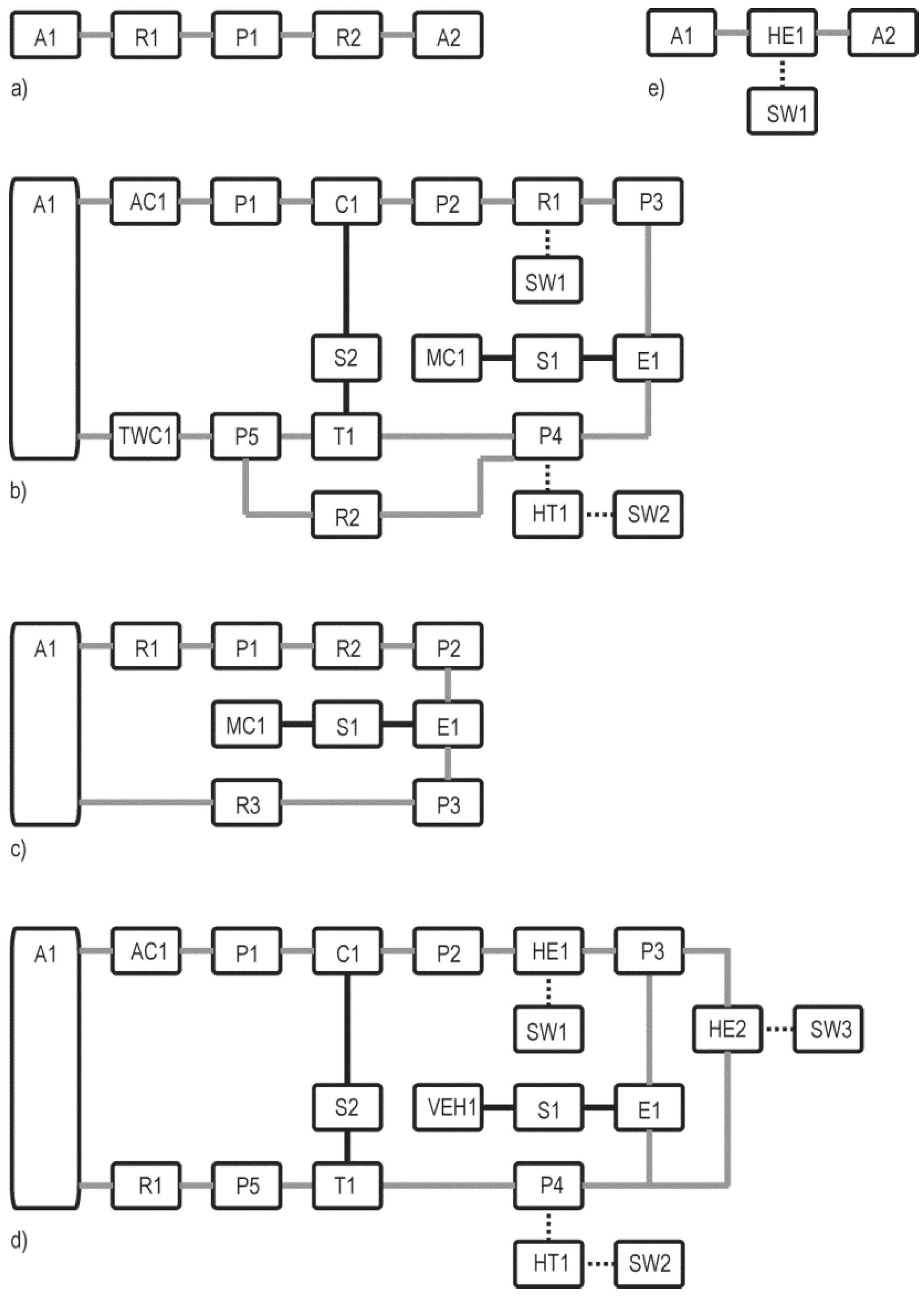
Figure 2. Topologies of: (a) the serially connected A1-R1-P1-R2-A2 (A-Ambient, R-Restriction, P-Plenum); (b) the 1.6 l turbocharged direct-injection spark-ignition engine equipped with the throttle valve (R1) and the turbine waste-gate valve (R2) (AC-Air Cleaner, E-Engine Block, MC-Mechanical Consumer, S-Shaft, TWC-Three Way Catalytic converter); (c) the naturally aspired 1.6 l spark-ignition engine equipped with the throttle valve (R2); (d) the 1.4 l turbocharged, intercooled diesel engine with cooled external EGR (HE2) and variable turbine geometry (VEH-Vehicle); and (e) the serially connected gas path A1-HE1-A2 (HE-Heat Exchanger) with attached SW1 (SW-solid wall). Grey connections denote exchange of the fluid, black dotted connections denote heat transfer and black connections denote the exchange of mechanical energy.

The results in Figure 3 are calculated without considering the TMB, i.e., by applying Equation (16). In Figure 3a–c large oscillations in all the variables are observed for the R scheme when applying the time step of 0.25 ms. Severe oscillations of the parameters originate from the interacting effects of the geometrical parameters, large time steps and the quasi-steady flow model of the restrictions, i.e., inertial effects arising from the time variation of the mass flow are not considered in the transfer elements. This leads to stiff systems, as indicated by the very large value of the stiffness ratio that is evaluated in Appendix A. As a result, oscillations of the Mach number with amplitude up to 0.8 are observed between the end time steps, i.e., within 0.25 ms, which is not physically meaningful. As the system exhibits oscillatory behaviour if a time step of 0.25 ms is used, there are no differences in the results between the cases wLF and woLF ([7] and Section 2.2). This is because the pressure oscillations in all the calculated steps are larger than the pressure threshold for entering the laminar flow calculations [${\mathrm{\Pi }}_{tr}$ = 0.98—Equation (22)] and thus the laminar-flow-calculation region is not entered. Unlike the R scheme, the H scheme does not feature oscillatory behaviour for this numerically unstable case, but the values for the end time steps are very far from the numerically converged solution, which is shown in Figure 4c,d or also in Figure 3d–f for the cases wLF.

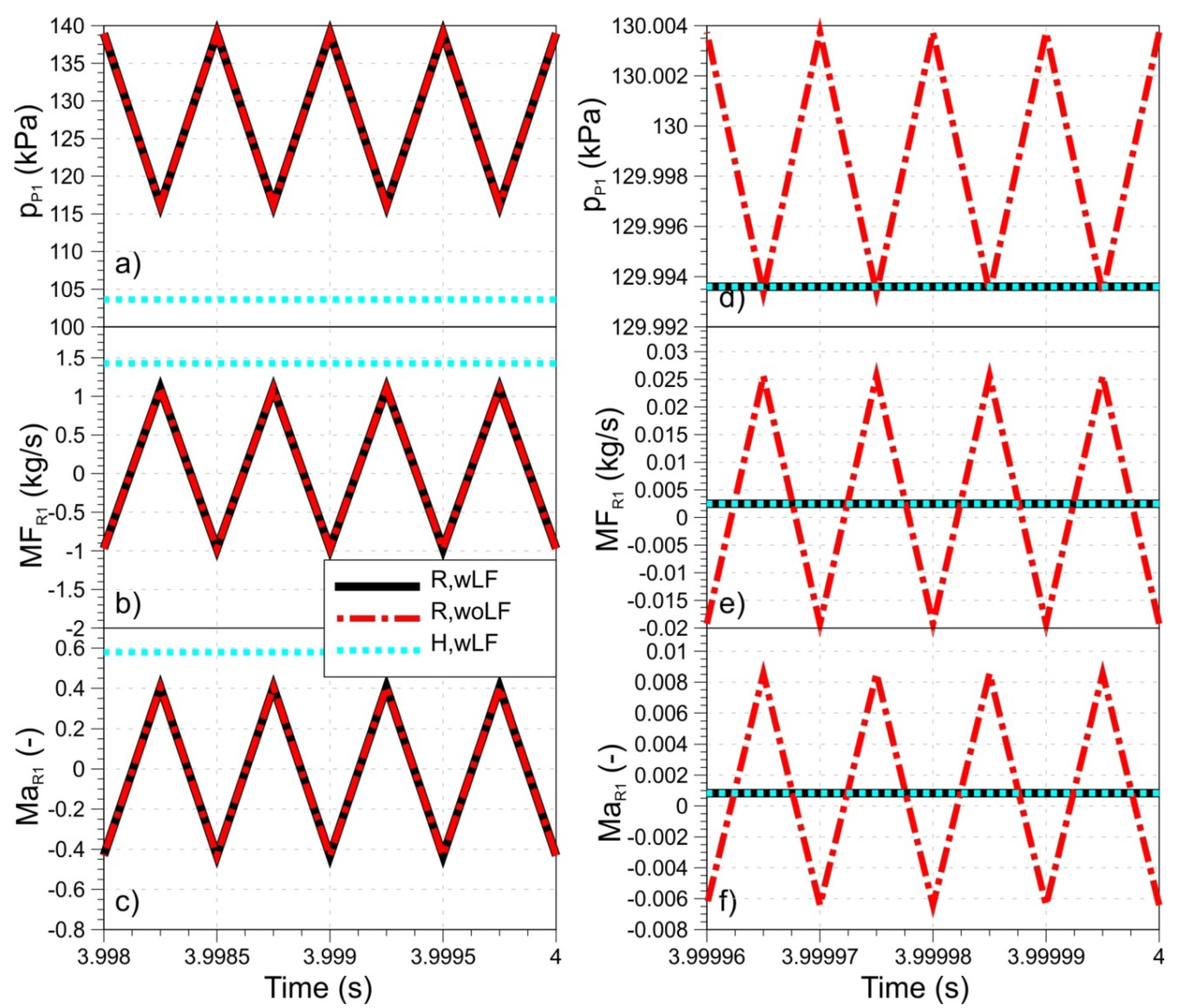
Figure 3. A1-R1-P1-R2-A2: pressure in P1 and the mass flow and the Mach number through the R1 for the time step 0.25 ms (a, b and c) and time step 0.005 ms (d, e and f). Results are calculated without considering the TMB for Ralston (R) and Heun (H) scheme. Results with (wLF) and without (woLF) assumed laminar flow conditions for very small pressure ratios are compared.

Figure 3. A1-R1-P1-R2-A2: pressure in P1 and the mass flow and the Mach number through the R1 for the time step 0.25 ms (a, b and c) and time step 0.005 ms (d, e and f). Results are calculated without considering the TMB for Ralston (R) and Heun (H) scheme. Results with (wLF) and without (woLF) assumed laminar flow conditions for very small pressure ratios are compared.

Figure 4. A1-R1-P1-R2-A2: pressure in P1 and mass flow through R1 for the time step 0.25 ms (a and b) and time step 0.005 ms (c and d). Results are calculated considering the TMB for Ralston (R) and Heun (H) scheme. Results with (wLF) and without (woLF) assumed laminar flow conditions for very small pressure ratios are compared.

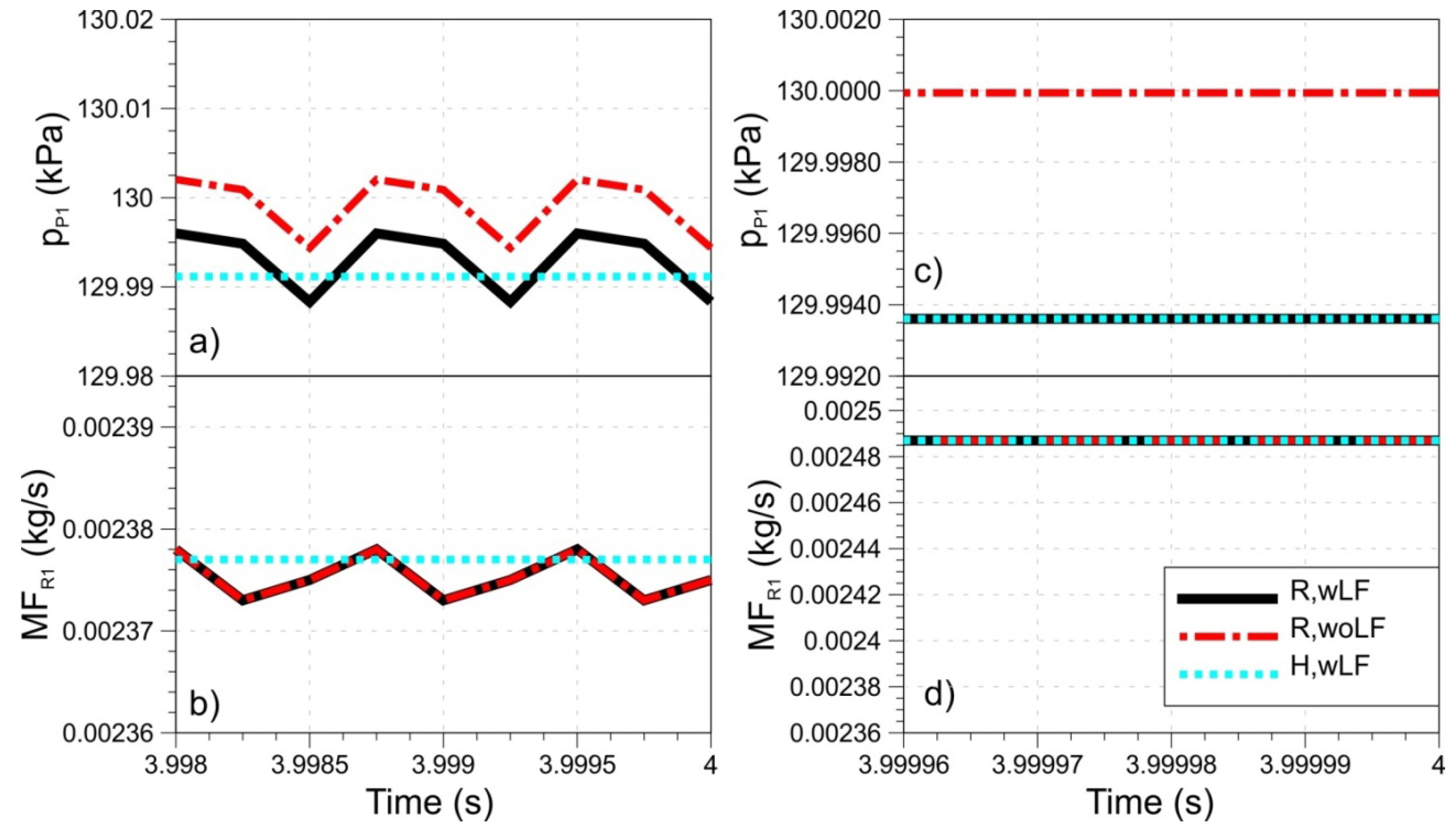
Figure 4. A1-R1-P1-R2-A2: pressure in P1 and mass flow through R1 for the time step 0.25 ms (a and b) and time step 0.005 ms (c and d). Results are calculated considering the TMB for Ralston (R) and Heun (H) scheme. Results with (wLF) and without (woLF) assumed laminar flow conditions for very small pressure ratios are compared.

With the time step reduced to 0.005 ms it is clear that the quality of the results has improved significantly for the case wLF as the stability of the system is enhanced under these conditions. Figure 3d–f show that for both integration schemes all the results are stable and identical for the case wLF. However, the maximum time step that still provides oscillation-free results is 0.05 ms for the R scheme, which does not comply with the realtime constraint. For the case woLF and the integration time step 0.005 ms oscillations of the pressure in the P1 are still observed; however, their amplitudes decrease with the decreasing time step, as discernible from the comparison of Figure 3a,d. Although the value of the pressure in P1 is very close to the correct value for the case woLF (Figure 3d) and the pressure oscillations in P1 are very small, it is clear that the pressure in P1 still features values that are higher than the upstream pressure in A1 for particular integration steps. This causes problems of flow reversals through the R1, which is shown in Figure 3e,f for the case woLF. Unphysical backflows between plenums with different species concentrations can cause problems when the flow signal from such a restriction is used as a controller input to steer, for example, the fuelling, since the mass-flow signal can be wrong even after filtering.

Figure 4 shows the results for the same configuration with the considered TMB. To ensure the same flow characteristics for the restriction as those shown in Figure 3, the flow through the restriction is modelled by Equation (32). The length of the restriction is generally not given; therefore, it is assumed that the length of the gas column (L) is equal to three hydraulic diameters of the cross-sectional area of the restriction. Figure 4 shows the pressure in P1 and the mass flow through R1 for the time step 0.25 ms (Figure 4a,b) and time step 0.005 ms (Figure 4c,d).

The stability analysis presented in Appendix A indicates that the addition of the gas columns with relatively short lengths can significantly reduce the stiffness of the system within the modelling framework applied in this paper. Therefore, unlike for the case without the TMB, no mass-flow reversals are observed in Figure 4b for a large integration time step of 0.25 ms. It is discernible that the pressure in P1 still reaches values that are higher than the upstream pressure in A1 for the scheme R and the case woLF. However, due to the consideration of the flow history and due to the consideration of the inertial effects arising from the time variation of the mass flow, pressure overshoots do not result in mass-flow reversals but only in a variation of the slope of the mass-flow trace [Equation (32)]. Variations of the slope of the mass-flow trace are also observed for the R scheme and consideration of wLF. It is clear that the mass flows coincide well for scheme R and the cases wLF and woLF, whereas a slightly smaller pressure in P1 is predicted in the case R,wLF. The trend observed with the R scheme is correct, as in the case wLF laminar flow conditions were assumed for the pressure ratios larger than ${\mathrm{\Pi }}_{tr}$ = 0.98 [Equation (22)] and thus a slightly larger pressure drop is needed to drive similar mass flow as in the case woLF (more details are given in [7]). In addition, it can be observed that both schemes R and H yield similar results for this integration increment. It is also discernible from the figure that for the integration time step of 0.005 ms the results are fully stable and that there are absolutely no oscillations of the mass flow through R1 and of the pressure in P1 for all the solution methods. Again, the same difference in pressure P1 is observed for the cases wLF and woLF due to the modified flow characteristics of the inflow boundary. These results clearly indicate that consideration of the TMB significantly contributes to the stability of the simulation system, which is particularly pronounced for larger integration time steps. This conclusion is also confirmed by the stability analysis presented in Appendix A.

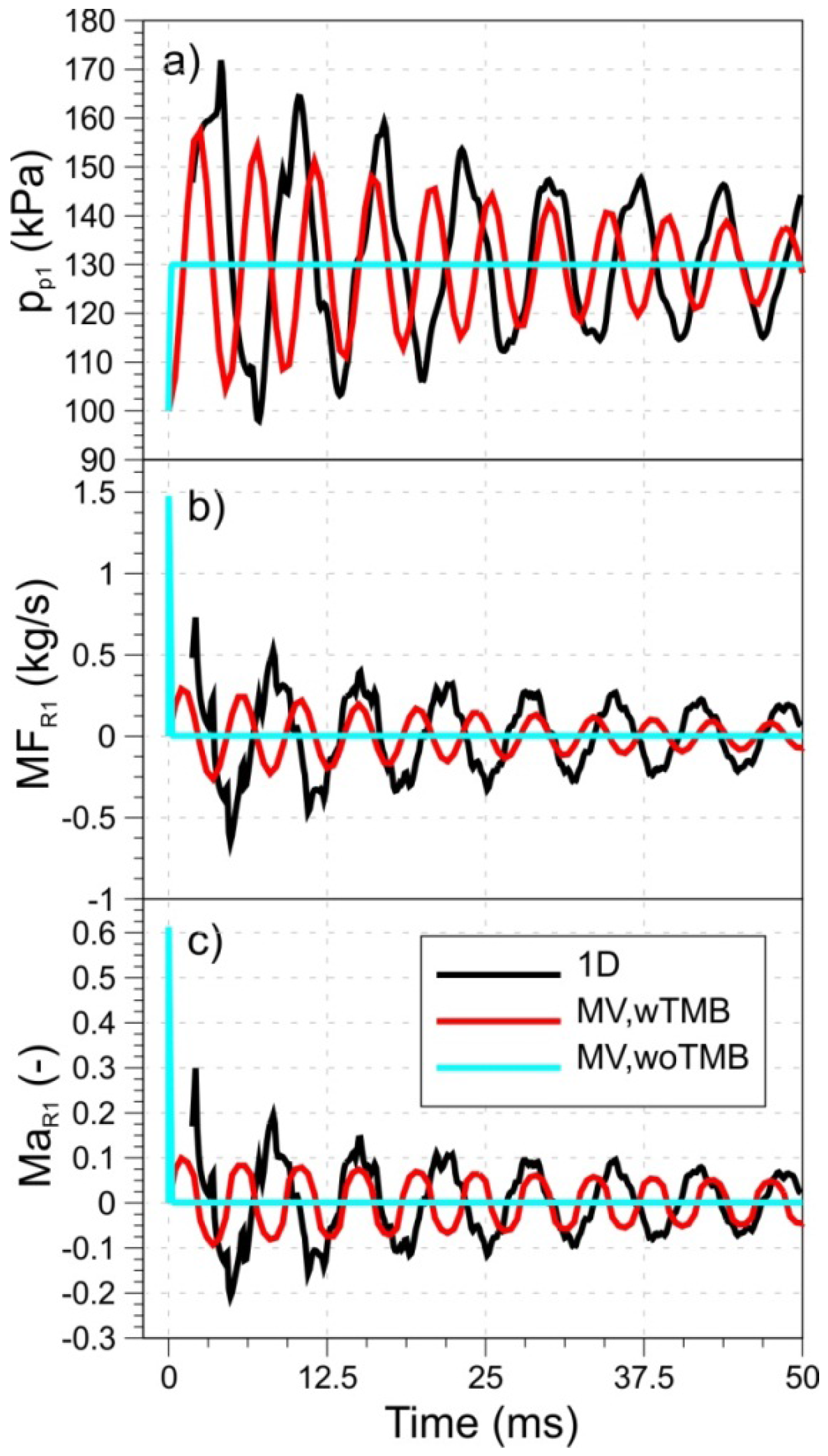
It is also meaningful to analyse the first part of the transient after time t₀ = 0 s for the same configuration, i.e., Figure 2a, and the same boundary and initial conditions. Figure 5 shows a comparison of the transient results for the first 50 ms. These results are calculated with: (a) the mean-value model without the TMB (MV,woTMB—time step of 0.005 ms was used); (b) the mean-value model with the TMB (MV,wTMB—time step of 0.5 ms was used); and (c) the commercial 1D simulation tool AVL BOOST [32] that is capable of capturing the wave dynamics in pipes (1D). Both results of the mean-value model were calculated using the R scheme and by considering the wLF. In the 1D simulation the same value of L was used as in the case of the MV,wTMB. The length L was discretized with 96 cells in the 1D model.

In the model without the TMB (MV,woTMB) mass flow (Figure 5b) and thus Mach number (Figure 5c) increase instantaneously to a very high value as this approach does not consider inertial effects arising from the time variation of the mass flow. Consequently, the pressure in P1 (Figure 5a) reaches a steady-state value nearly instantly in this case, since the cross-section of R1 is relatively large related to the volume of P1. In this numerically stable case, all parameters remain constant after this initial transient phase.

On the other hand, the results predicted by the 1D simulation tool reveal physically meaningful flow evolution in R1 and pressure oscillations in P1. Due to the spatial 1D discretization, 1D simulation tool resolves for wave dynamics in the R1. This means that at t₀ the pressure wave starts traveling from the boundary towards the P1 thereby accelerating the flow. After reaching the P1, the pressure wave is reflected at the open end as the rarefaction wave. This complex interaction of the pressure waves in R1 that drive the mass flow can be seen in highly dynamical traces of the mass flow and Mach number for the 1D case (Figure 5b,c). As a result, a highly oscillating pressure is characteristic for P1 (Figure 5c). It can be observed that pressure in P1 frequently reaches higher values compared to the pressure at the boundary, i.e., A1, which is the consequence of combined inertial effects arising from the time variation of the mass flow and wave dynamics. The former effect namely increases the pressure due to inertial forces that are needed to decelerate the flow.

Figure 5. A1-R1-P1-R2-A2: traces of (a) pressure in P1 and (b) the mass flow and (c) the Mach number through the middle of the R1 calculated with: (1) the mean-value model without the TMB (MV,woTMB); (2) the mean-value model with the TMB (MV,wTMB); and (3) the 1D simulation tool capable of capturing the wave dynamics in the pipes (1D).

Figure 5. A1-R1-P1-R2-A2: traces of (a) pressure in P1 and (b) the mass flow and (c) the Mach number through the middle of the R1 calculated with: (1) the mean-value model without the TMB (MV,woTMB); (2) the mean-value model with the TMB (MV,wTMB); and (3) the 1D simulation tool capable of capturing the wave dynamics in the pipes (1D).

Figure 5 shows that consideration of the TMB also makes it possible to model pressure pulses in the P1, which is related to the inertial effects arising from the time variation of the mass flow that are inherent to Equations (30) and (32). Here it is worth recalling that TMB approach relies on a single momentum equation applied to the complete transfer element, whereas in the 1D model, R1 is discretized with 96 cells. Therefore, results of the 1D and MV,wTMB models do not coincide fully as 1D model considers also wave dynamics in addition to the consideration of the inertial effects arising from the time variation of the mass flow. This difference is discernible through the following phenomena. Mass flow and thus Mach number in R1 as well as resulting pressure in P1 feature more pronounced dynamics in the 1D model as wave propagation phenomena are superimposed on the mass flow variation pattern driven by the inertial effects arising from the time variation of the mass flow. Therefore also frequencies of the oscillations of all parameters do not coincide fully as in the MV,wTMB case frequency is mainly defined by the pipe parameters and the pressure difference [Equation (32)] as well as by the volume of P1, whereas in the 1D case it is also influenced by wave dynamics. Although 1D models feature a more profound modelling depth, it is promising that the pressure pulses modelled with consideration of the TMB mimic similar trends. If desired, frequency of the pulses might be tuned by varying L in Equation (30) or (32). This example shows that consideration of the TMB makes it possible to model an additional dynamic effect of the system within the mean-value framework. These effects are for example of particular importance after sudden openings of the throttle valve.

5.2. Turbocharged Engine Example

In this section an experimentally validated model of a series production 1.6 L turbocharged direct-injection spark-ignition engine equipped with a throttle, a turbine with waste-gate valve and a camshaft phasing of the intake valves is analysed (Figure 2b). In this engine model heat transfer is considered in the exhaust manifold (P4) and in the throttle (R1), the latter also acting as the intercooler to optimize the computational expenses of the engine model. For the TMB case it was again assumed that the length of the gas column (L) is equal to three hydraulic diameters of the cross-sectional area of the restriction.

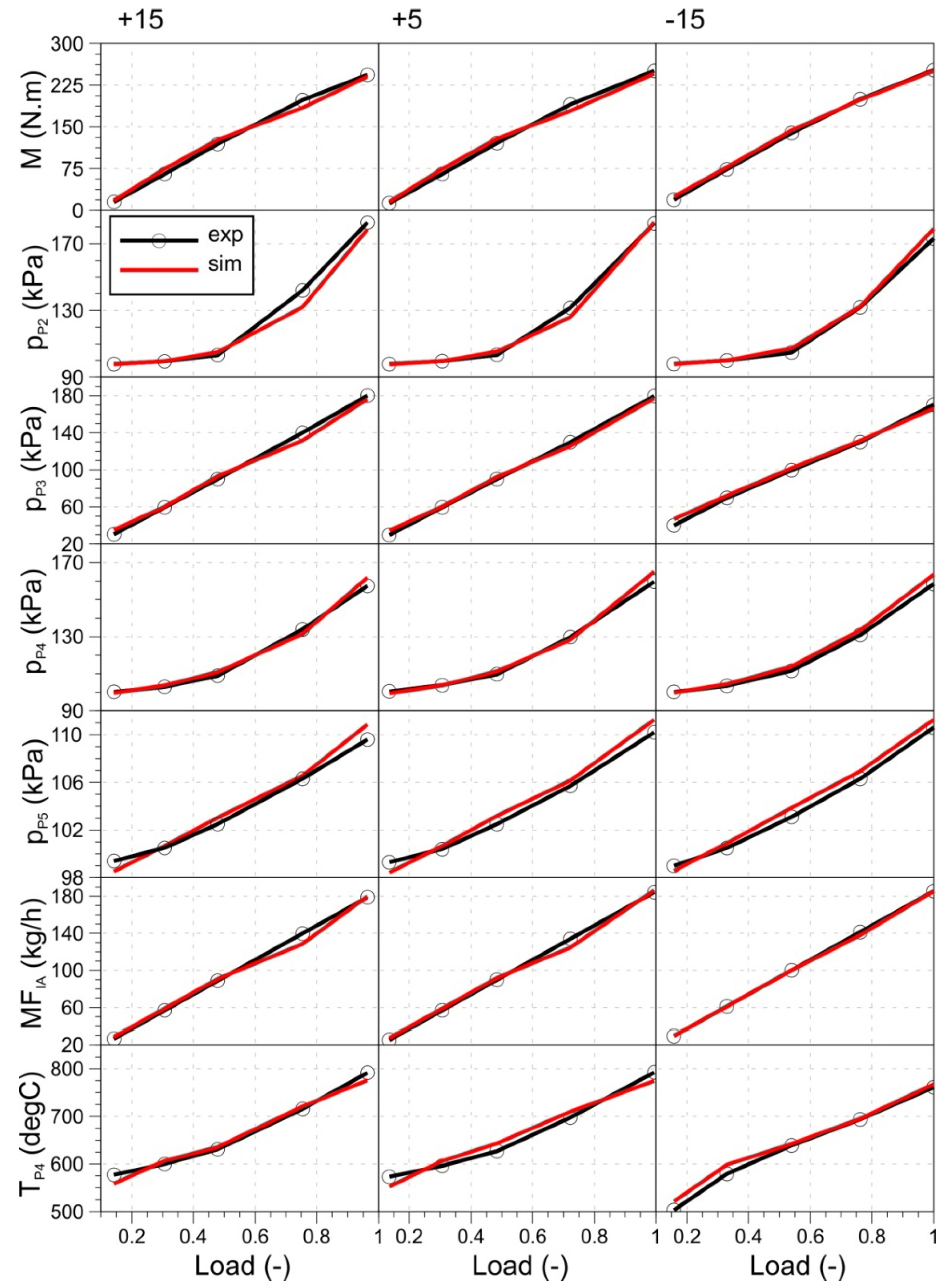
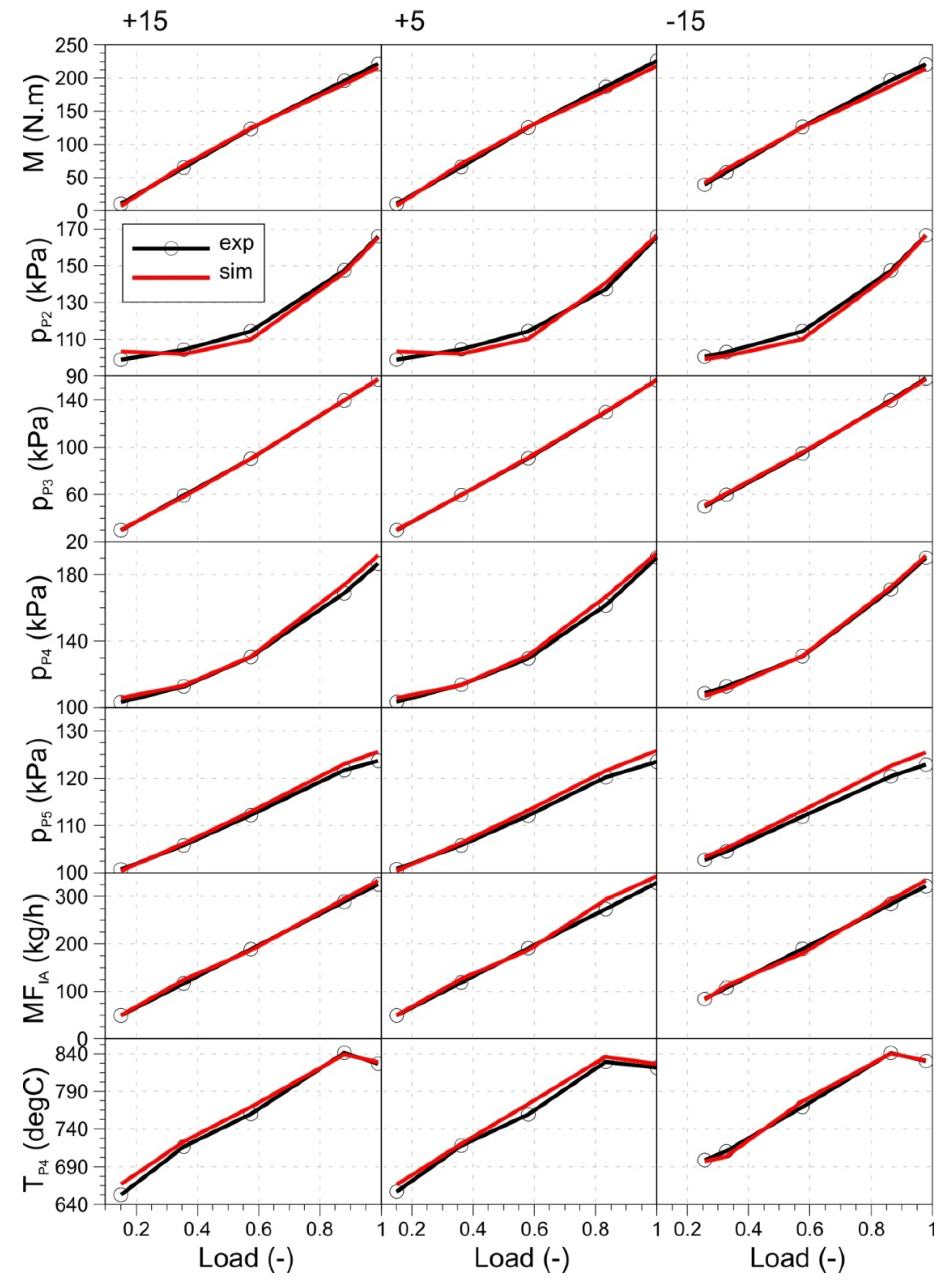
The surrogate engine-block model is embedded in the overall gas path model as a transfer element, which calculates mass, enthalpy and species fluxes as well as the engine torque with trained surrogate models (Figure 2b). The training of the models is done via Relevance Vector Machines [33] using experimental data. Each such surrogate model features different input variables and can thus be used very flexible. The air mass flow surrogate features the following inputs: engine speed, intake manifold pressure and camshaft phasing of the intake valve. Exhaust enthalpy and torque surrogate features the following inputs: engine speed, air mass flow and spark advance. Exhaust species flows were balanced considering mass flows of air and fuel. All engine models analysed in this paper are transient and thus steady-state operation was achieved by running the model for sufficient time at constant speed and load until convergence of the observed parameters was achieved. In the analysed case a simple mechanical consumer is therefore attached to the engine to ensure that the engine runs at a steady speed. The experimental validation of the model is presented in Appendix B.

A full-load operating point at 3000 rpm was analysed to show the stability of both mean-value approaches (with and without the TMB), since full-load cases represent the most severe test for the stability of the model due to low pressure ratios across the throttle. At a numerically stable operating point the model with and the model without the TMB return identical results. The maximum time step that allows an evaluation of stable results if the TMB is not considered is 1.3 ms for the R and 1.1 ms for the H scheme. For larger time steps, stability issues in terms of mass-flow reversals through the throttle, i.e., R1, were observed. If the TMB is considered stable results are obtained with a much larger time step of 4.5 ms for the R and 3.9 for the H scheme. It should be noted that the difference in the maximum time steps for the case when the TMB is considered or the case when the TMB is not considered decreases at part loads where the throttle is only partially opened, since in this case the pressure ratio across R1 is increased and the mass flow is reduced. However, consideration of the TMB always enables the use of larger integration time steps and thus shorter computational times.

The CPU time to calculate one complete integration step on a single core of the Intel i7 950 3.07 GHz processor is 0.258 ms (R) and 0.189 ms (H) for the case with the TMB and 0.209 ms (R) and 0.146 ms (H) for the case without the TMB. The difference between the cases with and without the TMB arises from the extra computational load associated with the more complex computation procedure when the TMB is considered. At this point it should be noted that the computational time of the heat exchanger routine is very similar with and without a consideration of the TMB; however, more operations are needed when evaluating the restriction when the TMB is considered as given in Section 2.2 and Section 2.3. Based on the above facts it can be concluded that much faster computational times can be achieved when considering the TMB, since it enables utilization of significantly larger integration time steps at only slightly increased CPU time needed to calculate one complete integration step. For the analysed case the ratio between the real-time factors (RT = CPU time/physical time) of the cases with and without the TMB, i.e., RT_wTMB/RT_woTMB, equals 0.356 for the R and 0.366 for the H scheme.

5.3. Naturally Aspired Engine Example

The naturally aspired engine model (Figure 2c) is derived from the turbocharged model presented in Section 5.2 by omitting turbocharging components and adequately simplifying the engine gas path topology while retaining the engine-block model. This example is analysed to expose the impact of including the compressor and the turbine components on the maximum time steps of the engine model, which are imposed by the stability criteria.

The full-load operating point at 3000 rpm was also analysed to maintain consistency with the analysis in the previous section. Like in Section 5.2, the stability issues of the naturally aspired engine are also indicated by the mass-flow reversals through the throttle, i.e., R2. Again, at a numerically stable operating point the model with and the model without the TMB give identical results. The maximum time step that allows an evaluation of stable results if the TMB is not considered is 0.4 ms for R and 0.3 ms for H scheme. If the TMB is considered stable results are again obtained with a much larger time step of 2.9 ms for R and 1.6 ms for the H scheme.

It is evident that maximum time steps of the naturally aspired engine are much shorter compared to the ones of the turbocharged engine analysed in the previous section. This is mainly related to the application of the turbocharger. Typically, intake or exhaust plenum and related transfer elements are the most prone to instabilities. In the case of the turbocharged engine the compressor forces and the turbine restricts the flow significantly more than the wide-open transfer elements where no mechanical work is added to or extracted from the flow, e.g., throttle, heat exchanger, air cleaner or the exhaust after-treatment devices. Therefore, simulation models of the turbocharged engine typically allow for larger integration time steps compared to similar naturally aspired engines.

The CPU time to calculate one complete integration step of a naturally aspired engine on a single core of the Intel i7 950 3.07 GHz processor is 0.13 ms (R) and 0.09 ms (H) for the case with the TMB and 0.1 ms (R) and 0.075 ms (H) for the case without the TMB. Again, the difference arises from the extra computational load associated with the more complex computation procedure when the TMB is considered. In this case the ratio between real-time factors for the cases with and without the TMB, i.e., RT_wTMB/RT_woTMB, equals 0.18 for the R and 0.23 for the H scheme, and thus the model with the TMB again allows for significantly faster computational times.

5.4. Transient Engine Example

In this section an experimentally validated model of a series production 1.4 L turbocharged, intercooled, diesel engine with a cooled external EGR and a variable turbine geometry is analysed (Figure 2d). In this case engine block-model features input of the fuel injection instead of the spark timing and camshaft phasing of the intake valve is not considered as engine features constant valve timings. In this engine model the intercooler and the EGR cooler that also acts as the EGR valve are modelled with heat transfer elements to ensure that both elements feature correct lengths. The engine powers a 1.3-ton vehicle that is equipped with a 6-speed manual gearbox. The vehicle is modelled by a longitudinal vehicle model that consists of the following driveline components: clutch, gearbox, final gear and differential, brakes, wheels and chassis. The complete engine and vehicle model is a forward-facing model. The results are shown for segments of the NEDC, where vehicle is driven on a chassis dynamometer. All results related to the transient engine operation were calculated using the R scheme and an integration time step of 1ms to avoid differences due to different integration time steps. This integration time step ensures numerical stability for both models, i.e., with and without the TMB. Due to the fact that the computational expenses of the heat exchanger are similar in the case with [Equation (30)] and associated equations] and without [Equations (25)–(27)] the TMB the computational time of the case with the TMB was only 1% longer over the complete NEDC compared to the case without the TMB.

Comparison of the results with and without consideration of the TMB is of particular importance, since consideration of the TMB is aimed at improving stability of the engine plant model while simultaneously preserving a high degree of its dynamic characteristics. Therefore it is intended to prove that results of both models are very similar for the integration time step that ensures numerical stability for both models, whereas the model with consideration of the TMB certainly possesses the potential to retain numerical stability also at larger integration increments as analysed in the previous sections. Here it is worth recalling that diesel engine analysed in this section does not feature any variable flow restrictions in the intake manifold, which might provoke effects presented in Figure 5.

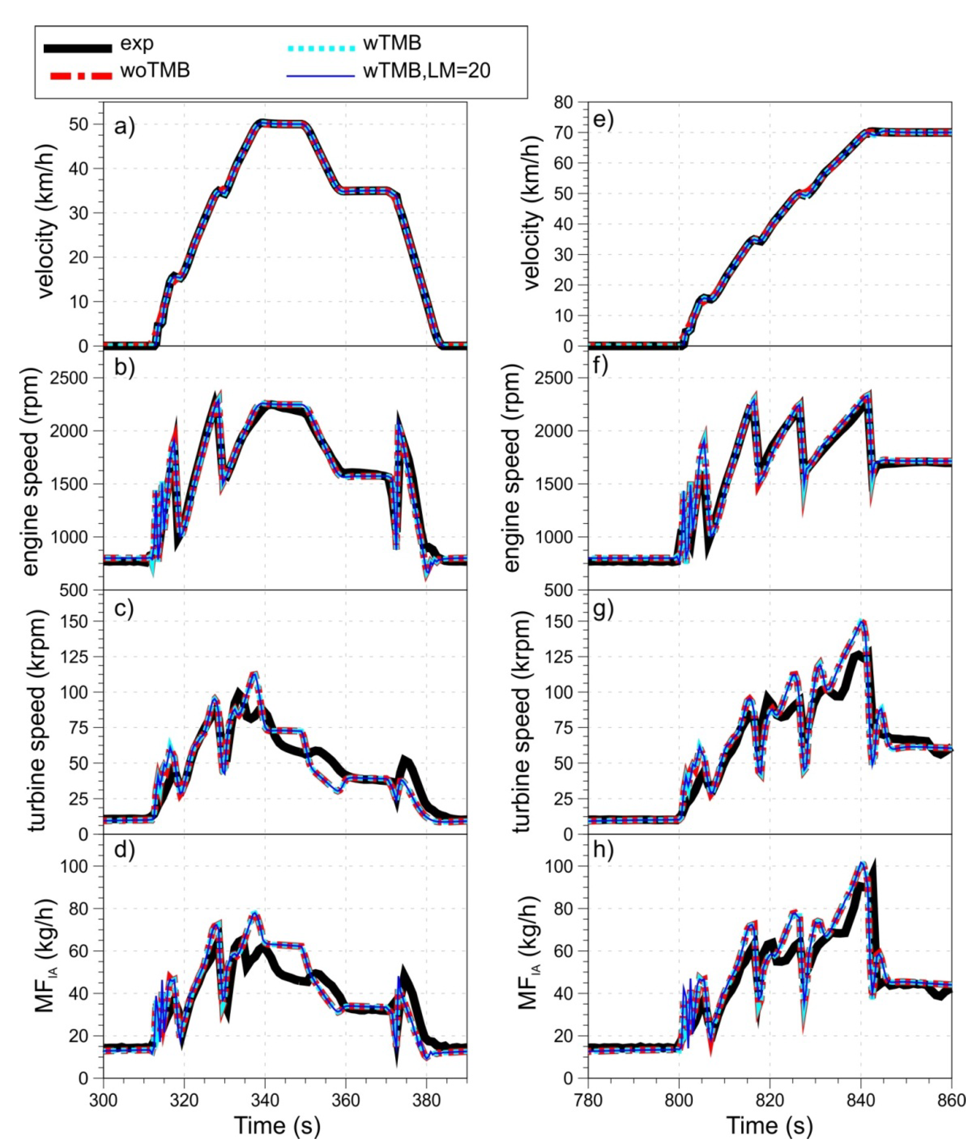
Figure 6 shows comparison between the experimental data and the simulation results without (woTMB) and with (wTMB) consideration of the TMB. An additional case, where all the lengths in the transfer elements were multiplied by an excessively high factor of 20 (wTMB,LM = 20), is also shown in the figure to demonstrate the influences of the increased inertial effects arising from the time variation of the mass flow on the engine results. It is clear from the figure that all the simulation results agree relatively well with the experimental results. The minor differences can mainly be explained by two facts. First, a simplified controller model that mimics the functionality of the real controller was used to control the engine. Although the applied controller works relatively well it does not feature all the functionality of the real engine controller, which certainly leads to some discrepancies between the experimental and the simulation results. Second, the real driver and the driver model do not behave identically, which leads to differences in the engine input and thus these discrepancies are added to the ones arising from the simplified controller model.

Figure 6. Results of the two NEDC segments showing a comparison of the experimental results (exp) to the results without the TMB (woTMB), with the TMB (wTMB) and with the TMB where all the lengths in the transfer elements were multiplied by an excessively high factor of 20 (wTMB,LM = 20) for vehicle velocity (a–e), engine speed (b–f), turbine, i.e., turbocharger speed (c–g) and intake mass flow (d–h).

Figure 6. Results of the two NEDC segments showing a comparison of the experimental results (exp) to the results without the TMB (woTMB), with the TMB (wTMB) and with the TMB where all the lengths in the transfer elements were multiplied by an excessively high factor of 20 (wTMB,LM = 20) for vehicle velocity (a–e), engine speed (b–f), turbine, i.e., turbocharger speed (c–g) and intake mass flow (d–h).

More important in the light of the topic presented in the paper is the fact that all the simulation results, i.e., those without and those with the TMB, coincide nearly perfectly for all the engine parameters. This can be explained by analysing the response times that are presented in Figure 5 and Figure A3 (Appendix C). There it is shown that for the geometrical characteristics of the components that are in the range of those used in the automotive application, the typical response times, due to consideration of the TMB, are of the order of a few milliseconds. Due to the fact that the typical response times of the engine manifolds, i.e., the plenums, are approximately two orders of magnitude longer, it is not even possible to observe any differences due to excessive prolongation of the elements, i.e., the case wTMB,LM = 20, on the time scale used in Figure 6.

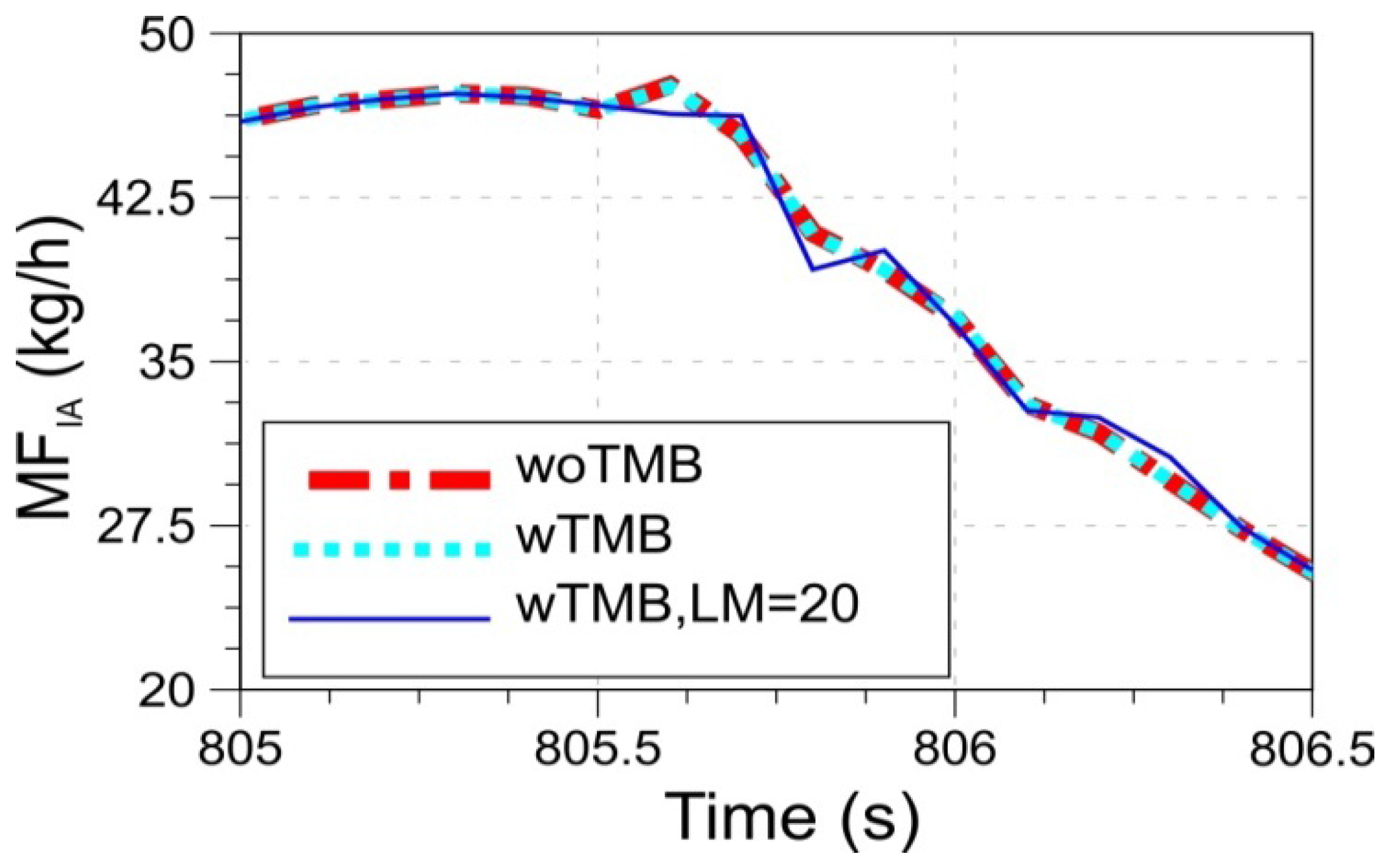
Only if a zoom-in into the segment of the gear shift from the first to the second gear (around second 805.5) is analysed (Figure 7) can some minor differences between simulation results be observed. In this interval the engine speed and thus also the mass flow change significantly due to the gear shift (Figure 6). Figure 7 indicates that up to the gear shift the results of all the models coincide, perfectly. Moreover, the results of the cases woTMB and wTMB also coincide perfectly throughout the complete transient phase, since the response time due to a consideration of the TMB is much smaller compared to the one of the plenum dynamics when realistic component lengths are considered. If the elements are excessively prolonged (wTMB,LM = 20) their response time is increased, whereas prolonged lengths also increase the amplitudes of the pressure fluctuations during fast transients. This is caused by the fact that in long elements more time is needed to accelerate the gas column with the same pressure difference leading to a lower frequency and a higher amplitude of the mass-flow oscillations. This phenomenon can be explained by a combined consideration of Equation (30) [or also Equation (32)] and Figure 5. These small, low-frequency, mass-flow oscillations can be observed in the fast transient region for the case wTMB,LM = 20.

Figure 7. Zoom-in into the segment of the NEDC, which exposes minor differences of the intake mass flow calculated with the wTMB,LM = 20 compared to ones calculated with the woTMB and wTMB.

Figure 7. Zoom-in into the segment of the NEDC, which exposes minor differences of the intake mass flow calculated with the wTMB,LM = 20 compared to ones calculated with the woTMB and wTMB.

Transient results thus indicate that a consideration of the TMB preserves dynamic characteristic of the engine model as the response times of the elements due to a consideration of the TMB are significantly below the response times of the engine manifolds within the framework of the MVEMs. Results also indicate that it is possible to slightly prolong the lengths of the elements without notably influencing dynamic characteristic of the model if this is needed to improve the stability of the model. However, these prolongations should certainly not be excessive. These results confirm that enhanced stability of the engine model is preferably achieved with the application of the TMB, as alternative frequently used technique that relies on increasing volumes of the plenums (rationale can be deduced from Appendix A) more significantly alters dynamic characteristic of the engine model.

6. Conclusions

The analytical framework of a novel approach to modelling the flow through the transfer elements of MVEMs is presented. In addition to the analytical rationale of the approach its applicability is confirmed by illustrative numerical models. It is shown in the paper that consideration of the TMB equation in the transfer elements of the MVEMs makes it possible to optimise the performance of the MVEMs as it enhances stability of the model. This fact results in two benefits arising through the consideration of the TMB: (1) it enables utilization of larger integration steps and thus increases computational speed of the model; and (2) for a comparable computational speed, i.e., comparable integration steps, it makes possible to model smaller plenums, which improves the fidelity of the simulation model. It was confirmed in the paper that the consideration of the TMB preserves dynamic characteristic of the engine model, which is of high importance in transient engine simulations. In addition, the consideration of the TMB can enable more adequate modelling of the highly transient phenomena in the engine gas path components within the mean-value modelling framework, since a more realistic description of the inertial effects more closely resembles the phenomena in the physical model.