1. Introduction
The attempt to fully understand the mechanics of extraction of energy from tidal currents is a challenging engineering problem. Conventional tidal stream energy devices take the form of an axial flow turbine using hydrofoils that generate lift and drag. Two aspects need to be considered: the effect of the flow on the turbine and the effect of the turbine on the flow field.
We may regard the torque that drives the rotation of the turbine as a function of the hydrodynamic forces that arise due to relative motion between the fluid and the rotating blades. Describing this relative motion, and thereby estimating the hydrodynamic forces, is therefore the primary requirement of a numerical scheme that models a tidal stream turbine (TST). One CFD approach is to utilise a moving reference frame containing the rotating turbine blades, which we describe in this paper. Difficulties in implementing this scheme may occur at the boundary of the moving part of the mesh, which manifests itself as a pressure discontinuity. More computationally-efficient schemes treat the rotor as an actuator disk, blade element disk or actuator line. These schemes are also discussed, with a focus on the blade element disk approach, which we refer to as BEM-CFD (blade element momentum-CFD). Finally, the least computationally-intensive numerical scheme is a blade element momentum theory (BEMT) approach, which is widely used for the analysis of propellers and other rotors. In this scheme, the flow field is assumed, and the computation reduces to a 1D treatment of the blade elements, comparing tabulated lift and drag coefficients with axial and rotational induction factors.
The BEMT scheme is computationally very fast, for instance running a tip speed ratio (TSR) sweep (roughly 400 individual simulations) in plug flow requires only around twenty minutes on a desktop computer, and can be used to study in detail time-varying effects, such as the effects of waves and rotor control strategies. By contrast, a TSR sweep in the BEM-CFD model takes around five days on a 32-core cluster. CPU times for coastal area models vary significantly based on the scale and resolution of the scenario being investigated.
The principal difficulty in validating these schemes is the lack of field data. Several sets of results are in the literature based on experiments with relatively small diameter rotors. Calculation of the Reynolds number based on the blade chord length shows that Reynolds numbers are significantly lower than those found in typical datasets for aerofoils in air [
1]. Computationally-efficient schemes, such as the BEMT and BEM-CFD approaches, rely on pre-determined lift and drag data and, thus, can only capture the effects of changes in sectional properties (e.g., as a result of biofouling or pitting) if these data are altered. We present a sensitivity study of these effects and propose some solutions to improve such schemes.
CFD models can be used to investigate the second aspect in the near-field: wake characteristics, recovery and interaction can all be modelled. Larger scale changes can be determined using coastal area models that can predict changes over hundreds of kilometres with much lower spatial resolution.
2. BEMT
The basic theory of BEMT is widely described in the literature [
2,
3], so we do not go into detail here. Briefly, one may describe the principle of the approach as reconciling two different models of a horizontal-axis turbine: a blade element (BE) model that treats the turbine as a collection of foil sections generating lift and drag forces in response to the oncoming flow and a momentum theory (MT) model that treats the turbine as a series of annular elements that absorb linear momentum (representing the slowing-down of the current due to the turbine) and impart angular momentum (representing the swirl induced in the turbine wake).
Two parameters are defined that capture the salient details in both models, and we obtain our solution by determining the values of these parameters that bring the two models into closest agreement. Our BEMT code [
4] incorporates several extensions to the classical theory, including tip/hub losses, high induction effects [
5] and the ability to model an arbitrary inflow. Here, we present its ability to capture the sensitivity of turbine performance to small changes in the hydrodynamic properties of the blade profiles.
We begin by considering three rotors for which experimental results have already been published. These turbines will be referred to by the institute at which the experimental work has been carried out. Thus, we have the rotors designed by Cardiff University [
6] and tested in the recirculating flume at Liverpool, which are reported in [
7,
8]; the IFREMER turbine, reported in [
9]; and the Manchester turbine, reported in [
10,
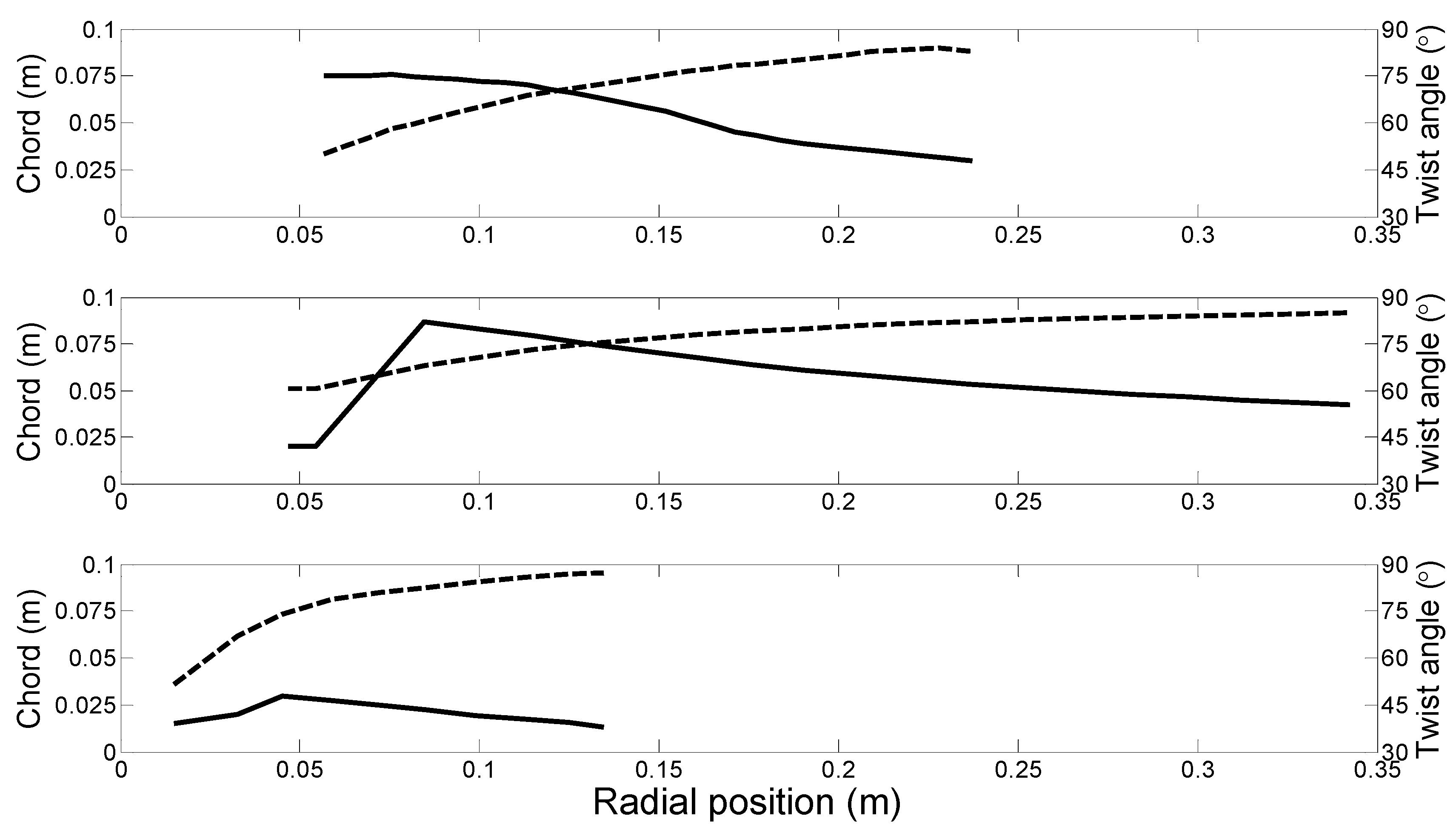
11]. All rotors have a three-bladed configuration, and the blade geometries for each are shown in
Figure 1.
Figure 1.
Blade geometries for the (top) Liverpool, (middle) IFREMER and (bottom) Manchester turbines. Chord length (distance from the section leading edge to the trailing edge) is shown with solid lines and the twist angle with dashed lines (90° meaning the section is parallel to the rotor plane).
Figure 1.
Blade geometries for the (top) Liverpool, (middle) IFREMER and (bottom) Manchester turbines. Chord length (distance from the section leading edge to the trailing edge) is shown with solid lines and the twist angle with dashed lines (90° meaning the section is parallel to the rotor plane).
The Liverpool rotor uses a Wortmann FX63-137 section for the entire blade length; the IFREMER rotor uses a NACA 63418 section; and the Manchester rotor uses a Göttingen 804 foil. BEMT relies on a table of lift and drag coefficients to calculate the forces generated by the blade elements, and the data for each of these foils were taken from different sources. The coefficients for the Wortmann foil were taken from a flume study carried out at Swansea [
12] at Re = 5 × 10
4; for the NACA 63418 section, data were taken from standard tables [
1] for moderate angles of attack with Re = 9 × 10
6, with flat-plate theory used for extreme angles of attack; for the Göttingen foil, data were taken from a wind tunnel study [
13] at Re = 3 × 10
4. Data for the Göttingen foil are much less complete than those for the other sections; additionally, the section stalls very abruptly and at an unusually low angle of 8°. To ensure a fast runtime, the data are not smoothed, and linear interpolation is used to estimate lift and drag between data points. As a result of the sparse data and the interpolation, the BEMT results contain many small discontinuities, since in many cases, a relatively small change in inflow angle results in a large jump in the lift and drag properties of the foil. This is also noticeable in the BEMT work carried out at Manchester, as can be seen in the studies that report their experimental results [
10].
As we mention above, the purpose of the work presented here is to investigate the sensitivity of turbine performance to small changes in the lift and drag properties of the hydrofoils used in the rotor blades. For each rotor, we calculated four sets of performance data: One with the original geometry, one with decreased lift (
i.e., C
L decreased by 10% at all inflow angles), one with increased drag (
i.e., C
D increased by 50% at all inflow angles) and one with both lift and drag altered. These cases are intended as a simple representation of the degradation of section performance due to factors such as biofouling or surface pitting due to cavitation, and the magnitude of the changes are in line with those found in experimental investigations [
14]. Note that an earlier numerical investigation by Batten
et al. [
15] treated drag in a similar fashion, but did not consider the effects of roughness on lift. These results are presented graphically in
Figure 2, along with experimental data for the IFREMER and Manchester turbines.
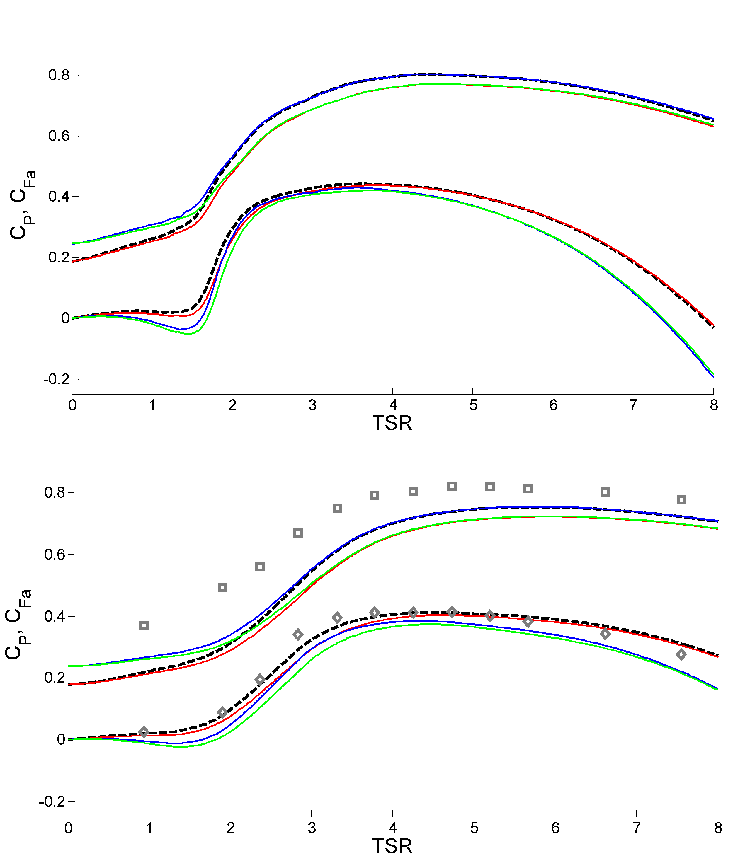
Figure 2.
Power (C
P) and axial force (C
Fa) coefficients for (top) Liverpool, (middle) IFREMER and (bottom) Manchester turbines. In all cases, the upper cluster of lines shows C
Fa, and the lower shows C
P. Black dashed lines show original turbine performance; red lines show the 90% C
L case; blue lines show the 150% C
D case; green lines show the combined lift decrease and drag increase case. Experimental results are also shown for the IFREMER and Manchester turbines (in grey), with data taken from [
9,
11], respectively. Note that for the range of TSR values investigated, both the Liverpool and Manchester turbines go beyond the freewheeling state (
i.e., C
P = 0); in a real turbine, this operating condition cannot be reached.
It is immediately apparent that there are few large changes in turbine performance as a result of lift/drag changes of this magnitude. This is reassuring from an operational point of view, as it implies that relatively small changes to the blade characteristics that may occur as a result of biofouling or blade erosion/pitting are unlikely to cause a large drop in performance.
The details of the performance changes vary between rotors: we tabulate the most important parameters in
Table 1. In C
P terms, the IFREMER rotor is more sensitive to lift/drag changes than the Liverpool rotor, although their C
Fa sensitivities are very similar. The Manchester rotor C
P drops more significantly with degradation of section performance, particularly when drag is increased. It should be remembered that the Manchester rotor was designed in order to replicate full-scale thrust characteristics, rather than power characteristics, and so, changes in its C
P curve are likely to be atypical. It is clear from this table, and from
Figure 1, that across all rotor geometries, C
P is more affected by an increase in sectional drag, whereas sectional lift has a greater influence on C
Fa.
It is not only the value of the optimum CP that is altered by these changes in blade profile properties, but also the TSR at which this optimum is attained. An increase in sectional drag coefficient always results in a downwards shift of the optimum TSR, while a decrease in lift has different effects: for the Manchester rotor, the optimum TSR shifts slightly downwards, but for the IFREMER and Liverpool rotors, the shift is upward. A sophisticated control scheme, then, may be able to use sensitivity analyses, such as those presented here, to partially compensate for blade degradation by altering the TSR at which the turbine is operated.
Table 1.
Changes to maximum power and thrust coefficients and optimum TSR for Liverpool, IFREMER and Manchester turbines in response to small changes in the lift and drag properties of blade sections.
Table 1.
Changes to maximum power and thrust coefficients and optimum TSR for Liverpool, IFREMER and Manchester turbines in response to small changes in the lift and drag properties of blade sections.
| | | Liverpool | IFREMER | Manchester |
|---|
| Max CP | Original | 0.4431 | 0.4122 | 0.3350 |
| CL − 10% | 0.4377 (−1.22%) | 0.4035 (−2.12%) | 0.3119 (−6.88%) |
| CD + 50% | 0.4287 (−3.26%) | 0.3848 (−6.66%) | 0.2157 (−35.62%) |
| Both | 0.4213 (−4.92%) | 0.3736 (−9.37%) | 0.1866 (−44.3%) |
| Max CFa | Original | 0.8018 | 0.7531 | 0.9761 |
| CL − 10% | 0.7707 (−3.88%) | 0.7224 (−4.07%) | 0.9175 (−6.00%) |
| CD + 50% | 0.8024 (+0.08%) | 0.7540 (+0.13%) | 0.9643 (−1.21%) |
| Both | 0.7714 (−3.79%) | 0.7234 (−3.95%) | 0.9185 (−5.90%) |
| Optimum TSR | Original | 3.64 | 4.52 | 4.64 |
| CL − 10% | 3.84 (+5.50%) | 4.62 (+2.21%) | 4.54 (−2.15%) |
| CD + 50% | 3.52 (−3.30%) | 4.32 (−4.42%) | 4.10 (−11.64%) |
| Both | 3.70 (+1.65%) | 4.50 (−0.44%) | 4.40 (−5.17%) |
We can also see that the agreement between the BEMT code’s predictions of the unmodified rotor performance and the experimental data for the IFREMER and Manchester turbines is good throughout the range of experimental TSR values. Taking the peak values as representative, for the Manchester results, power agrees to within 2.9% and thrust to within 3.0%; for the IFREMER turbine, power agrees to within 0.3%. The apparent exception is the axial force coefficient for the IFREMER turbine, but this discrepancy is attributable to the fact that the measured axial force included the force on the supporting structure and not simply the rotor disc itself. Despite this difference, it can nevertheless be seen that the trend of axial force’s dependence on TSR matches the experimental observations. Note that the IFREMER results have been corrected for blockage using the method of Glauert [
2]. In order to apply this correction, the power and thrust coefficients must correspond to the same TSR values; the experimental values provided by Stallard
et al [
11] do not satisfy this condition, and thus, the correction cannot be carried out in this case. However, the blockage in this experiment was only 2.5% and, thus, would not greatly alter the results reported. In fact, we can specify upper bounds on its influence for this blockage ratio: no C
Fa value would change by more than 1.4%, and no C
P value by more than 2.2%. Overall, the agreement between BEMT predictions and experimental results allows us to be confident in our numerical model.
3. CFD and BEM-CFD
The most complete computational model of a full-scale tidal turbine that can feasibly be run is a large eddy simulation (LES) [
16], although unsteady RANS remains more common [
17,
18]. Such a model will necessarily rely on a moving mesh to account for blade rotation. The moving boundary in the mesh may present difficulties, manifesting as a pressure discontinuity and greater computational costs. An alternative method is the BEM-CFD model in which the flow properties are resolved by interaction of the BEM and CFD methods [
19,
20,
21,
22]. As BEM by itself does not provide any useful information about the effect of a turbine in the far-field, we use CFD to resolve the full domain [
23]. In other words, the BEM method is used to model the turbine, and CFD is employed to model the flow properties elsewhere in the domain, thus giving us a time-averaged estimate of the turbine wake while significantly reducing the computational cost compared to a geometry-resolved CFD model. Here, we will present two sets of results from a BEM-CFD model validated against CFD and against experimental measurements.
We start by modelling a single tidal turbine configuration in both the BEM-CFD method and a blade-resolved geometry (BRG) CFD method. In the comparison between these two models, we are primarily interested in the velocity deficit in the turbine wake. An understanding of turbine wakes is vital if tidal turbines are to be deployed in arrays [
24] (as turbine wakes will inevitably impinge on other turbines located downstream), and such arrays are the only way tidal turbines can be economically viable [
25].
The CFD finite volume model is constructed and set up in ANSYS Fluent. This was provided by the Marine Energy Research Group of Cardiff University. The turbine used in this model is the based on the Liverpool rotor described in
Section 2, but scaled up to a diameter of 10 m. The details of this blade, including the performances and mesh details, are provided in [
6,
17,
18]. The computational domain has dimensions 506 m × 50 m × 50 m, in which the turbine is located 104 m from the inlet to allow the flow to settle before reaching the turbine. This domain is chosen based on the studies published previously, which have shown that with this distance from the side walls, there would be minimum effects from the boundary on the turbine [
6]. The inlet boundary condition is set as a uniform flow of 3.086 m/s (equivalent to six knots, a typical flow speed of a potential TST deployment site), and a no-slip condition is imposed at the bed and blade surfaces. For all of the side walls and the top of the domain, symmetry boundary conditions have been enforced. At the outlet boundary, a zero diffusion flux condition for all flow variables is imposed. The rotational speed of the blade was set to 2.25 rad∙s
−1 or TSR 3.64, the design optimum rotational speed for the rotor in normal operation. Note that this is identical to the optimum TSR found in BEMT simulations of the Liverpool rotor (see
Table 1). The zone that represents the rotation of the rotor is set to have a 17 m diameter and a 6 m width. The properties of the mesh for this model are discussed in detail in [
6].
An equivalent model has also been implemented using the BEM-CFD method. The domain geometry is the same and is meshed with 6.03 million tetrahedral elements. The mesh sizing for the both cases is different in the vicinity of the blades. Unstructured tetrahedral elements have been adopted in a way to be able to capture the geometry of the blade properly for the BRG-CFD model. The boundary conditions are the same as those used in the Fluent model. Rather than representing the geometry of the turbine directly as in the CFD model, we treat the rotor as a momentum source/sink in the domain based on the geometry and hydrodynamic properties of the blade. This BEM-CFD method has been validated in the previous research of the group, together with a mesh independence study [
25].
Both the BRG-CFD and BEM-CFD models employ a standard finite volume approach with a k-ε turbulence model. Note also that in both cases, we are modelling only the rotor itself: no support structure (nacelle, tower, etc.) is included. The rotors rotate clockwise in both models viewed from upstream.
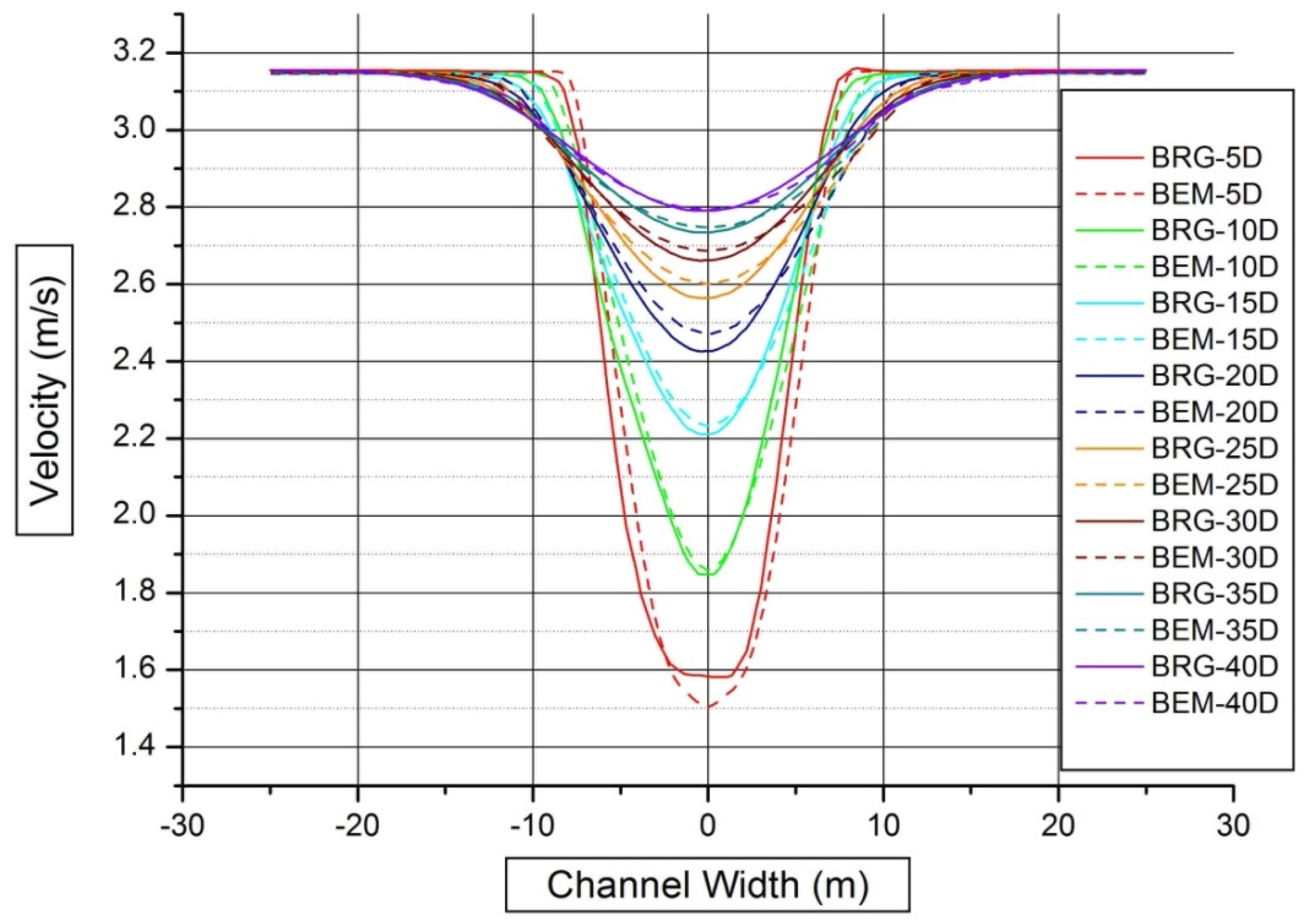
In
Figure 3, we compare the two models’ predictions of velocity deficit at five diameter (5D) intervals between the distances of 5D and 40D behind the turbine. The values are extracted along the horizontal line passing behind the turbine at the hub level. We see that the models agree well throughout most of the wake. Five diameters downstream of the rotor, the velocity has dropped by more than 50% in comparison to the inlet velocity, although on the centreline, the BRG predicts a higher wake velocity than the BEM-CFD. Further downstream, the wake profiles are very similar across the span of the domain, both in terms of the magnitude of velocity deficit and wake spreading. The results also show that the wake shape for the BEM-CFD method is symmetric, while the BRG method’s wake is slightly asymmetric. The lower minimum velocity observed in the BEM-CFD method could be linked to relative over-prediction of turbine power in the BEM-CFD method compared to the BRG model. Comparison of C
P and C
Fa for both models shows that the BEM-CFD method predicts a slightly higher C
P value of 0.44 compared to 0.40 for the BRG-CFD, and the C
Fa for the BEM-CFD and BRG-CFD is 0.81 and 0.83, respectively. The BRG-CFD results are published in [
18] and also have good agreement with the BEMT results shown in the top panel of
Figure 2. It should be borne in mind that for simplicity, this comparison is done in a uniform flow above a flat bed; in the real environment, non-uniform flows and sloped surfaces will influence the results [
9,
26].
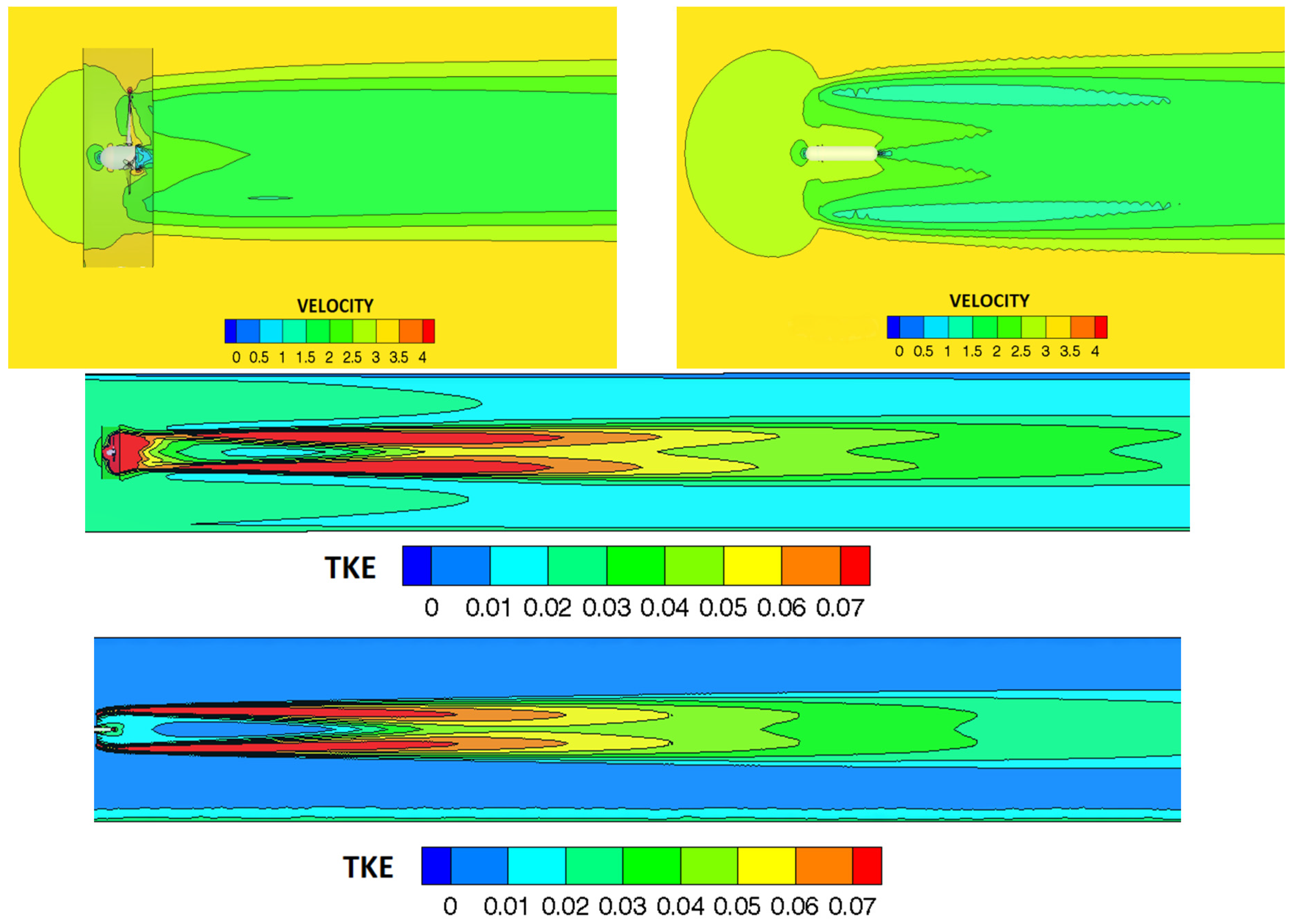
Figure 4 shows the velocity deficit and the turbulent kinetic energy for each of the models.
Figure 3.
Comparison of the velocity deficit in the rotor wake from BEM-CFD and blade-resolved geometry (BRG) models at a range of downstream locations.
Figure 3.
Comparison of the velocity deficit in the rotor wake from BEM-CFD and blade-resolved geometry (BRG) models at a range of downstream locations.
In addition to validating the BEM-CFD model against the BRG-CFD results, we have also carried out a comparison with experimental results carried out in the IFREMER flume, the same results used as one of the test cases for the BEMT simulations reported in
Section 2.
Figure 5 demonstrates that results from the BEM-CFD method match experimental measurements well, in comparison to
Figure 9a of [
9]. A comparison of BEM-CFD and BEMT methods is also conducted using the rotor geometry from the IFREMER experimental study.
Figure 6 and
Figure 7 demonstrate the coefficient of power and coefficient of axial thrust plotted against TSR. The results show that BEMT under-predicts power in comparison to BEM-CFD. This under-prediction is largest near the optimum, with the model predictions varying by 5.4%.
Figure 4.
Comparisons of the velocity deficit between BRG (top right) and BEM-CFD (top left) and between turbulent kinetic energy (TKE) for BRG (middle) and BEM-CFD (bottom) in the Cardiff 10-m rotor wake.
Figure 4.
Comparisons of the velocity deficit between BRG (top right) and BEM-CFD (top left) and between turbulent kinetic energy (TKE) for BRG (middle) and BEM-CFD (bottom) in the Cardiff 10-m rotor wake.
In comparing the BEMT, BEM-CFD and experimental results, it is important to bear in mind the effects of blockage and how this differs between the three cases. BEMT results always reflect a turbine operated in a theoretically perfect blockage-free state, whereas both experiments and CFD introduce a flow constriction (flume walls for experiment, domain boundaries for CFD) that forces more fluid through the turbine than in an equivalent unblocked condition. Thus, it is to be expected that we would find better agreement between BEMT and experiment when the blockage of the experiment is corrected, as is seen in the second panel of
Figure 2, but better agreement between BEM-CFD and experiment if this correction is not applied, as is seen in
Figure 7 and
Figure 8. A slight complication arises in that, although the BEM-CFD simulations replicated almost all of the conditions of the experiments reported in [
9], the mast on which the turbine was mounted was omitted for reasons of computational cost. The experimental measurements of thrust in fact included the drag on this mast, as well as the rotor thrust (as mentioned in
Section 2), which explains the offset between numerical predictions of thrust and the corresponding measured values. Furthermore, the additional thrust on the mast means that blockage was more significant in the experiments than the BEM-CFD simulations. Thus, the changes in the experimental power and thrust curves due to the correction are larger. This is why we have better agreement between unblocked experiment and BEMT, and between blocked experiment and blocked BEM-CFD, than we see between unblocked BEM-CFD and BEMT.
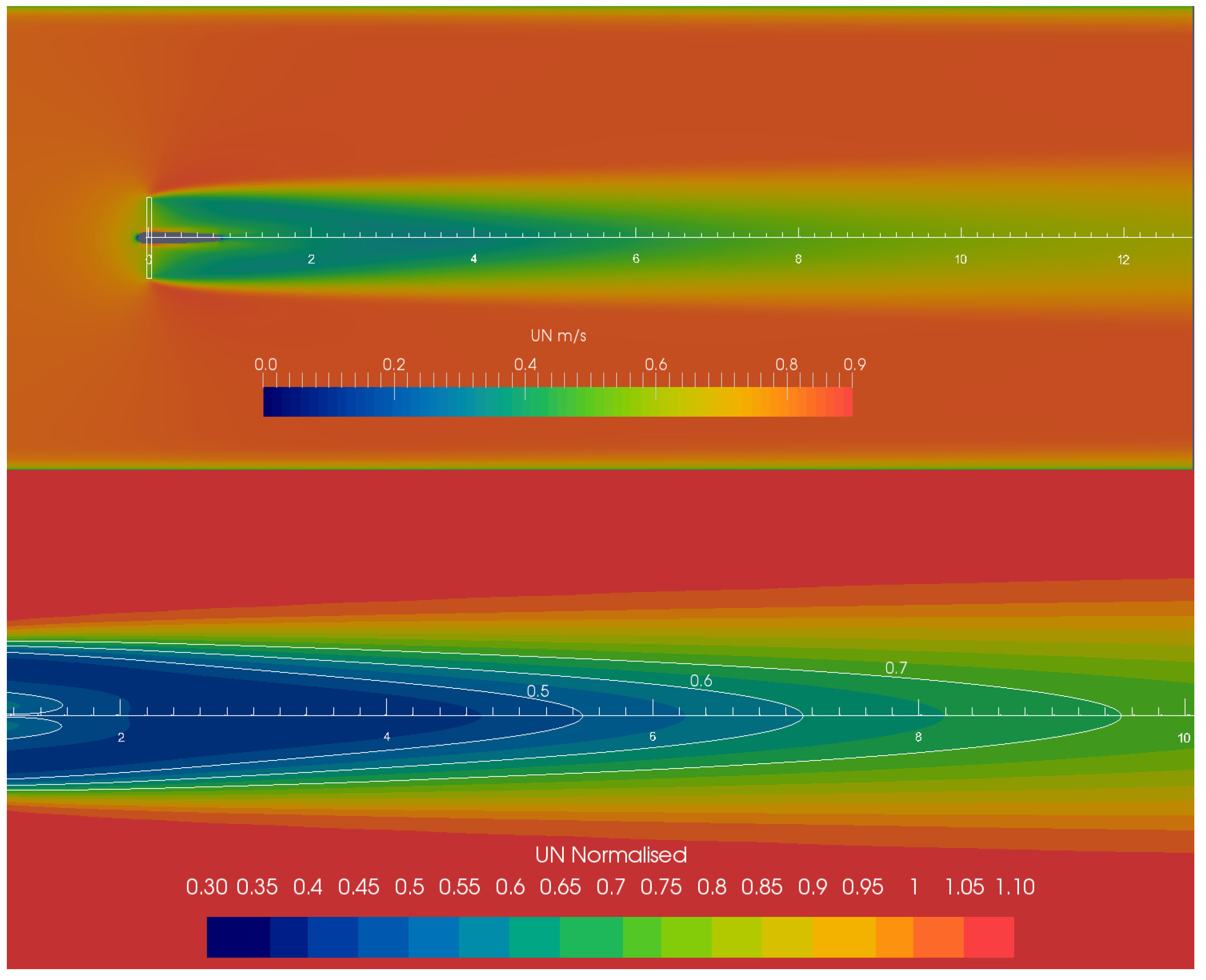
Figure 5.
BEM-CFD model of IFREMER wake characteristics: axial velocity slice taken at the hub centre. Free stream velocity is 0.8 m·s
−1; TSR is 3.67; and background turbulence intensity is set at 3%. The top panel shows the full wake to the end of the domain, while the bottom panel is staged to compare with
Figure 9a from [
9] and includes isolines at 0.5, 0.6 and 0.7 normalised axial velocity.
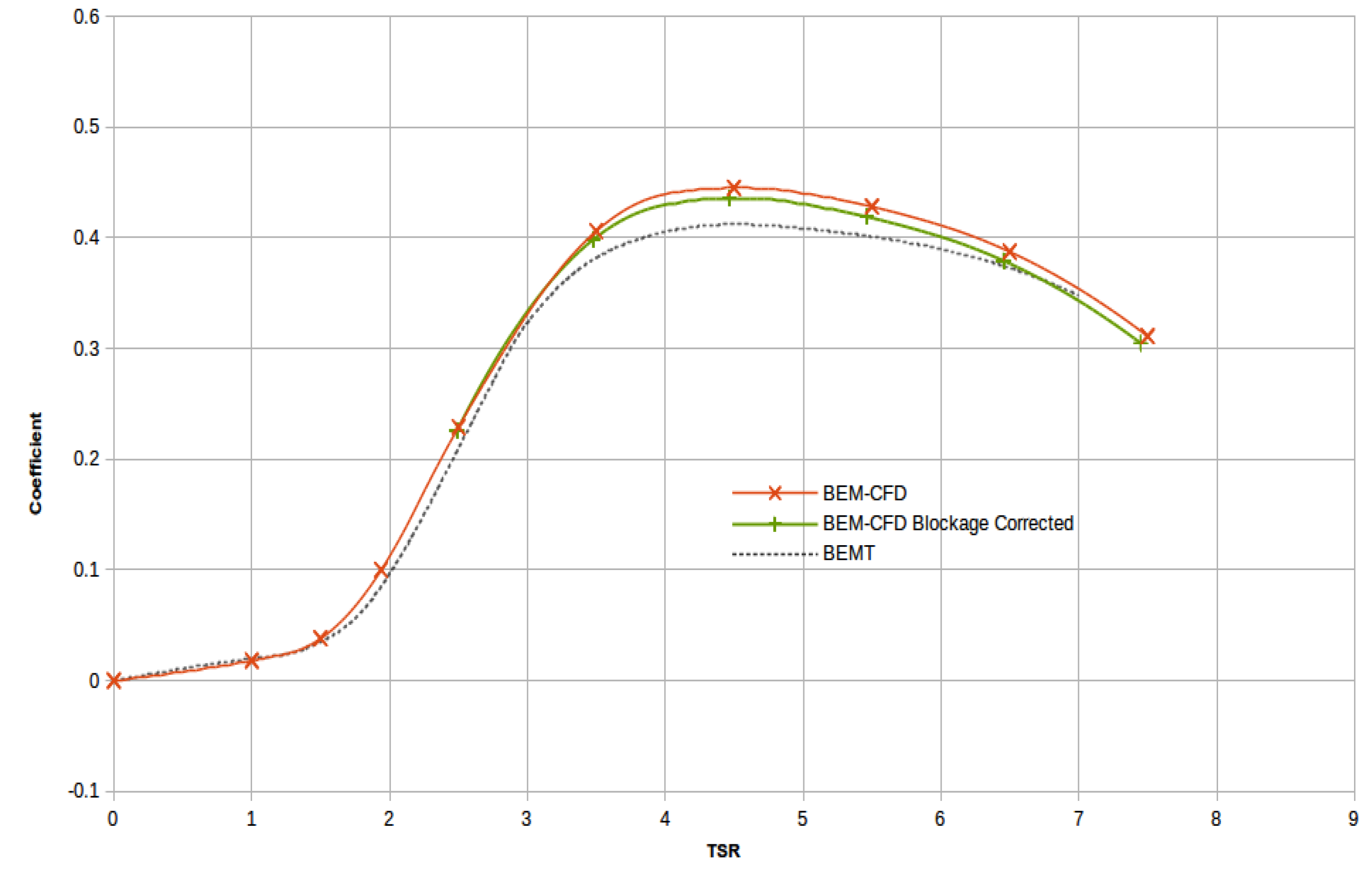
Figure 6.
Comparison of IFREMER rotor results for CP (coefficient of power) between BEM-CFD and BEMT for a range of TSRs. Blockage corrected BEM-CFD results are included for reference.
Figure 6.
Comparison of IFREMER rotor results for CP (coefficient of power) between BEM-CFD and BEMT for a range of TSRs. Blockage corrected BEM-CFD results are included for reference.
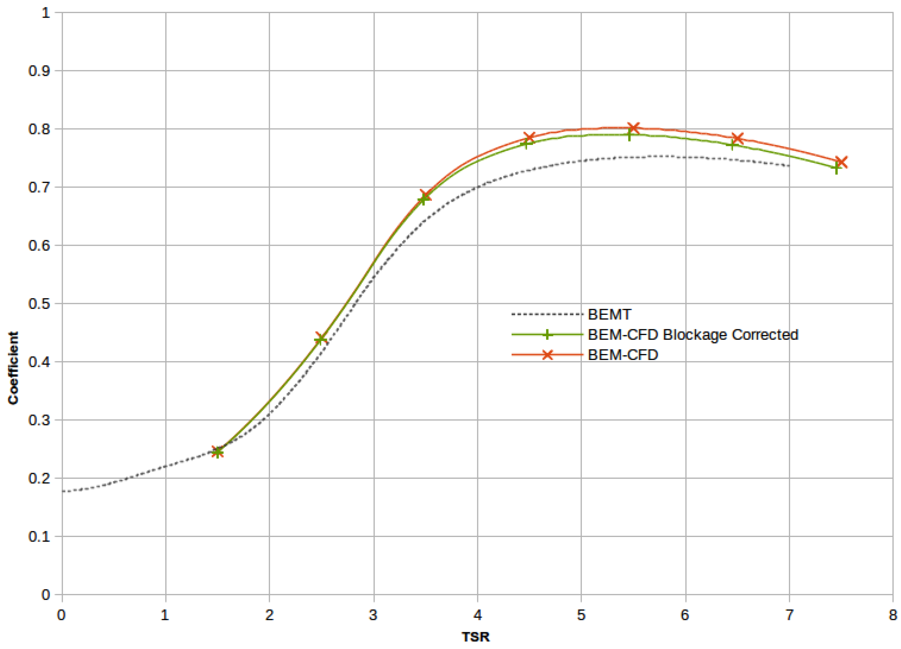
Figure 7.
Comparison of IFREMER rotor results for CFa (coefficient of axial thrust) between BEM-CFD and BEMT for a range of TSRs. Blockage-corrected BEM-CFD results are included for reference.
Figure 7.
Comparison of IFREMER rotor results for CFa (coefficient of axial thrust) between BEM-CFD and BEMT for a range of TSRs. Blockage-corrected BEM-CFD results are included for reference.
4. Coastal Area Modelling
While CFD and BEMT approaches are focused very much on the turbine itself, whether in terms of structural loading, blade performance or detailed wake structures and intra-array interactions, computational limitations mean that different techniques are required for the modelling of larger-scale impacts or for long time period simulations. Coastal area models are therefore used, which typically solve the shallow water equations in two or three dimensions. Horizontal meshes are either rectangular or, increasingly, unstructured, and models are either 2D depth averaged or, in the 3D case, cater to vertical resolution with a series of layers. Model domain sizes for coastal area models range from the order of 10 km for site-specific modelling to the order to 1000 km for shelf-scale studies of multiple arrays or far-field impacts. Simulation durations typically range from a single tidal cycle to more than a year, with time steps of seconds to minutes and output periods of minutes to hours. Coastal scale modelling typically investigates available resource [
27,
28] or the impacts of energy extraction on the wider environment for array or inter-array scenarios. Resource modelling is conducted to provide greater spatiotemporal coverage than is achieved with field measurements [
29].
Impacts on the hydrodynamic regime can be observed over a much larger area than covered by CFD. Hydrodynamic responses can be noticed on an ocean scale for tidal barrages and on a regional to shelf-sea scale for tidal stream turbines [
30,
31]. Changes to hydrodynamic regime can lead to second-order effects. Researchers have also investigated impacts on sediment transport and associated changes to morphology [
32,
33,
34,
35]. Wave-current interactions [
36] can also be an important process, both in affecting the tidal resource and the changes to currents impacting the wave climate [
37,
38,
39], the water quality [
40] or aquatic organisms. More recently, optimal siting for power production over a large area has been considered [
41].
A variety of methods have been used for the implementation of turbines in coastal array models: in two-dimensional models, the impact of turbines is often included as an additional component of bottom friction within the array footprint, either averaged over the whole array or as individual turbines [
33,
34,
42]. The value used is often based on actuator disk theory with correction factors applied when array scale extraction is considered [
43,
44]. In three-dimensional models, such an approach would give unrealistic vertical velocity profiles, and thus, an additional sink term must be introduced to the model [
35]. A review of the commonly-used methods is presented in [
45]. Many coastal area models only consider the reduction in momentum; however, the rotor also generates additional turbulence, which some studies have also included to increase the realism of the impact of turbines on flow. Roc
et al. [
46] show that excluding turbulence reduces the accuracy in the simulation of wake recovery; thrust only leads to a faster recovery of the wake than shown in measurements, while inclusion of turbulence matches measurements well.
Currently, few turbines are installed in the real world, and no turbine arrays have been deployed. This means that few full-scale data exist on the impact of turbines on flow in the natural environment, and what data do exist re commercially sensitive. Therefore, it is not currently possible to conduct full-scale model-measurement comparisons relevant to coastal area models. This means that the two options to increase confidence in turbine formulations in coastal area models are comparison with scaled experiments, e.g., [
47], or model-model comparison. In order to demonstrate the contrast between BEM-CFD and a coastal area model (Danish Hydraulic Institute’s MIKE3), the two techniques were used to model a simplified case of a fence of six turbines at an idealised headland. Such comparisons are useful to demonstrate the difference in outputs between the two techniques, to determine areas in which the coastal area model will give unrealistic results and to give credence to the simpler coastal area model approach given the lack of real full-scale turbine wake data available for model validation.
Both models use finite volume techniques to solve the incompressible Reynolds-averaged Navier–Stokes equations, but mesh resolution and turbine implementation is different. The other key differences are: the difference between time-stepping (coastal area model) and steady state (BEM-CFD) simulations; the free surface for the coastal area model; and that MIKE3 invokes the assumption of hydrostatic pressure, whereas the BEM-CFD considers dynamic pressure given the smaller mesh spacing. In the coastal area model, the Boussinesq assumption is invoked and turbulence catered to with eddy viscosity based on the Smagorinsky formulation. The BEM-CFD model used was that described in
Section 3, and the coastal area model used was MIKE3 by the Danish Hydraulic Institute [
48]. MIKE3 was chosen as the tested model, because it is a commercial piece of code regularly used in renewable energy applications.
The scenario tested in this paper was based on [
49] and the BEM-CFD case more fully described in [
25]. The domain was 770 m wide for both cases with the headland extending by 230 m. The offshore boundary was set to full slip condition in both cases. The bathymetry was set to be a constant 30 m, and the six turbines had a hub height of 15 m and a rotor diameter of 10 m. Turbine hub spacing was set at 20 m. The BEM-CFD case extended 450 m upstream and downstream of the headland centreline, whereas the coastal area model extended to 7000 m downstream. This difference is due to the lack of a similar boundary condition for the downstream boundary in the coastal area model compared to the BEM-CFD model. The BEM-CFD model implemented a zero pressure downstream boundary, whereas one could not specify this in the coastal area model, and hence, the extended domain with the same downstream boundary conditions as the upstream boundary. For both models, the upstream boundary was a plug flow with 3 m·s
−1 velocity parallel to the shoreline and a still water level of zero (hence, a water depth of 30 m). The BEM-CFD model has a fixed lid at the zero water level, whereas the coastal area model has a free surface apart from the specified level at the boundary. In both models, bed resistance is set to zero.
In both the coastal area model and BEM-CFD simulations, only the rotor was considered with no support structures or nacelles included. MIKE3 has an inbuilt turbine tool based on actuator disk theory [
38]. The drag force
FD is calculated as:
where ρ
w is the density of water, α is a correction factor that is equal to one in this study,
CD is the drag co-efficient,
Ae is the effective area of the turbine and
V is the velocity. A constant drag co-efficient was specified as 0.9, which was equivalent to the thrust coefficient reported from the BEM-CFD simulation results. This co-efficient varied between devices in the BEM-CFD results, and thus, the average value across the fence was used in the coastal area model. The drag force, calculated by Equation (1), is then used to implement a sink in the momentum equations using an extra source term. No additional turbulence is generated by the energy extraction process in the coastal area model. Conversely, the BEM-CFD mesh has sufficiently fine resolution to capture the turbulence generation [
26]. Full details of the representation of the turbines in the BEM-CFD model are described in
Section 3.
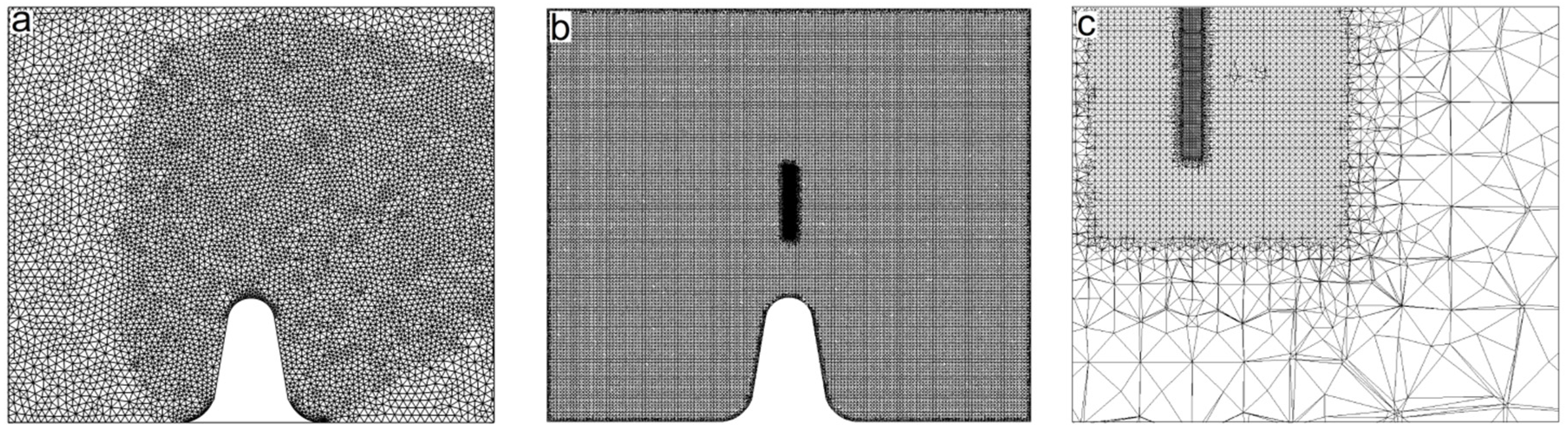
The meshes used are shown in
Figure 8 to demonstrate the difference in resolution. Since the BEM-CFD model is a fully-3D mesh, the figures show slices through the mesh at hub height, whereas the coastal area model uses a layered approach, and thus, the displayed mesh is the actual mesh. In the coastal area model, the turbines are implemented as sub-grid structures, and the triangular horizontal mesh in the fence region has an area of 68 m
2, such that a 10-m diameter rotor fits within one triangle. By contrast, the BEM-CFD model has 50,000 elements representing each rotor.
Figure 8.
Meshes used in the headland case example: (a) the coastal area model; (b) the BEM-CFD model; and (c) a close up of the BEM-CFD mesh showing the gradation to finer regions around the turbines.
Figure 8.
Meshes used in the headland case example: (a) the coastal area model; (b) the BEM-CFD model; and (c) a close up of the BEM-CFD mesh showing the gradation to finer regions around the turbines.
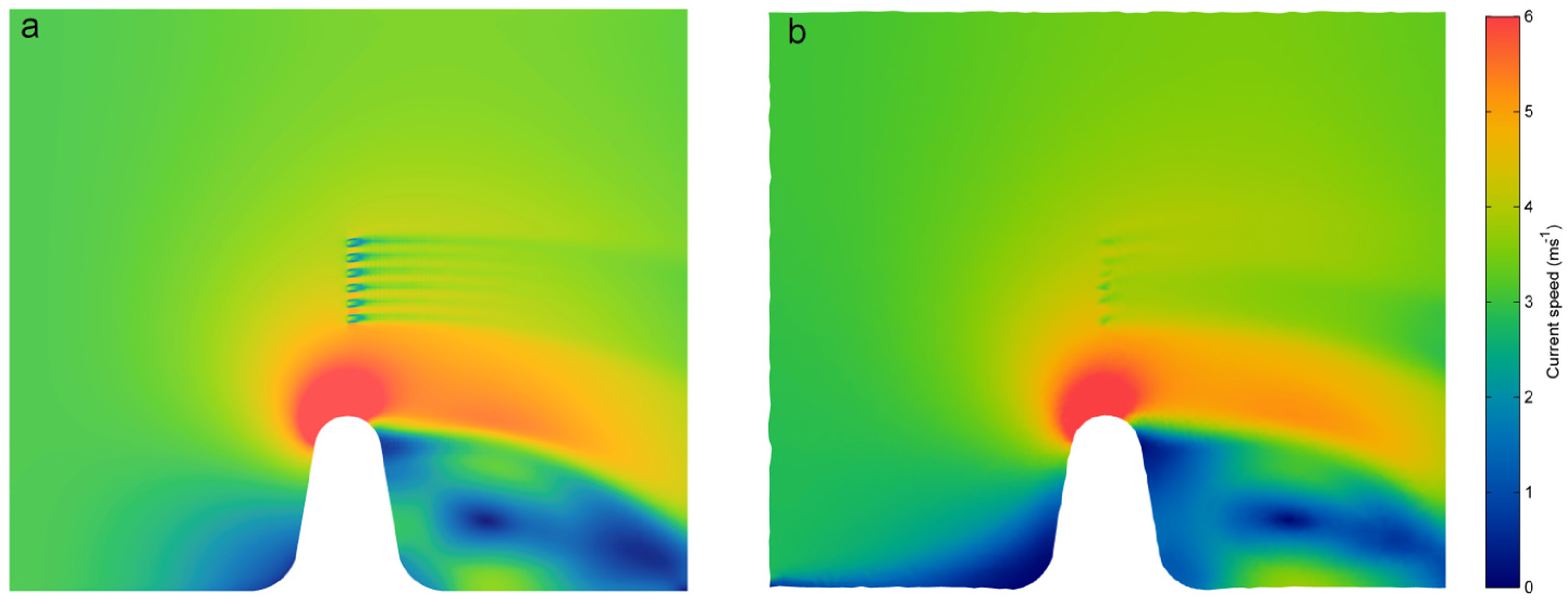
Figure 9 shows the velocity field at hub height for both simulations. Clearly, the BEM-CFD model resolves the turbine wakes in much greater detail; however, in the far-field, flows are similar.
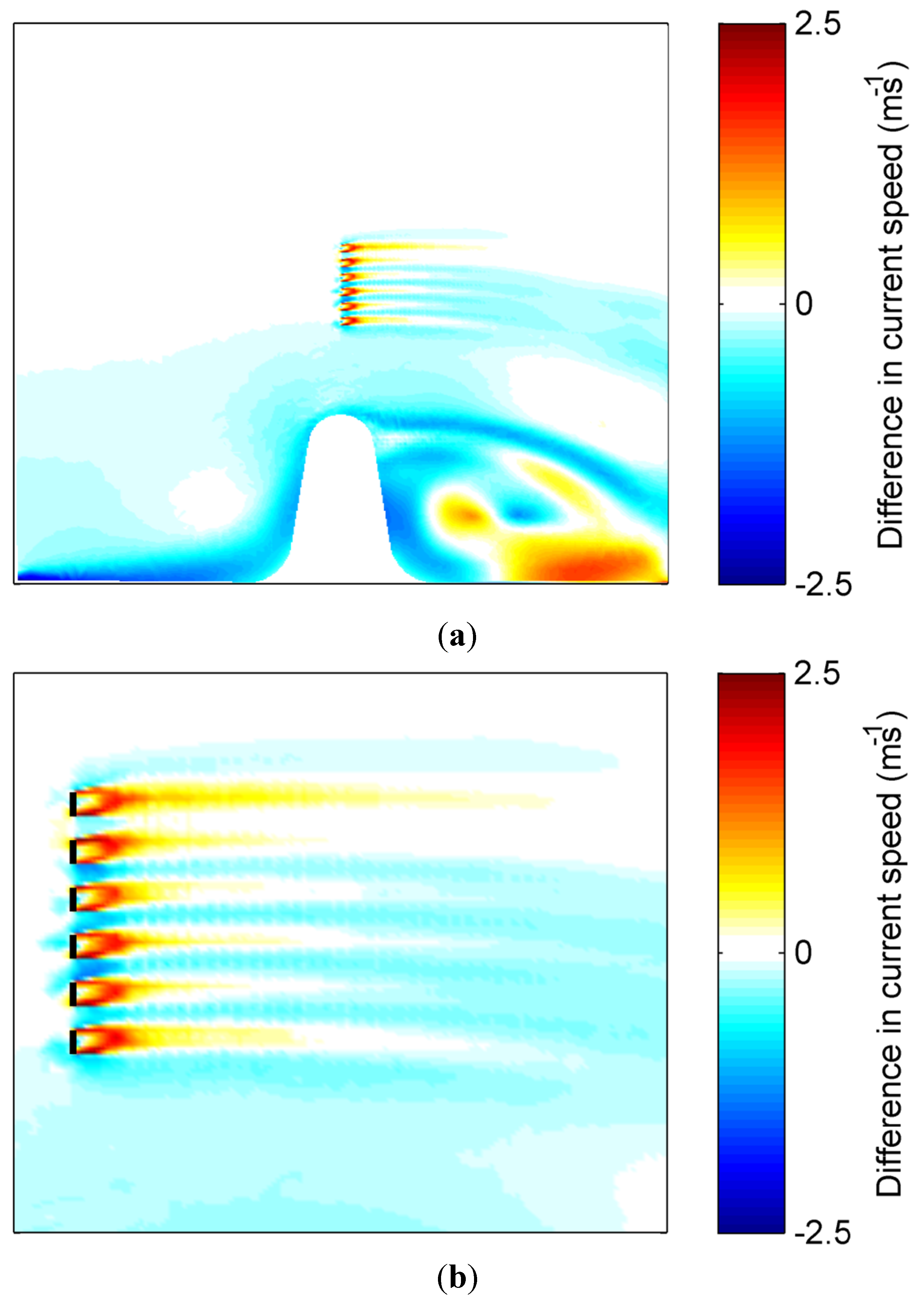
Figure 10 shows the difference in flow speeds between the two cases. Lower velocities are observable close to the land on the upstream side for the coastal area model. In both tests, the land boundary is specified as zero velocity; however, for the CFD case, the much finer mesh means that velocity can increase in greater proximity to the boundary. Within 1–2 cells away from the boundary, the coastal area model gives similar results. Flow velocities in the far-upstream and offshore of the turbine fence can be seen to be very similar. Flows between the headland and the turbine fence are slightly lower for the coastal area model than for the BEM-CFD. In this area, the difference in water level between the fixed lid of the BEM-CFD and the free surface of the coastal area model is greatest (
Figure 11).
The shape and location of the vortex in the lee of the headland is visually similar for the selected time step, although
Figure 10 shows that there are some large differences in magnitude. Comparison of a steady-state and time-varying model is somewhat arbitrary, since a method of selecting the appropriate time step to consider is not obvious. If the coastal area model is run for a long time period, a vortex develops and propagates downstream before a new vortex forms. Similar flow behaviour has been reported by [
45]. Therefore, in this case, the time step where visually the vortices looked similar was chosen so that differences in vortex location did not affect the wake structures.
Figure 9.
Horizontal flow fields for the headland fence case: The images show velocity magnitude at hub height from: (a) the BEM-CFD model; and (b) the coastal area model. Flow is from left to right in the images.
Figure 9.
Horizontal flow fields for the headland fence case: The images show velocity magnitude at hub height from: (a) the BEM-CFD model; and (b) the coastal area model. Flow is from left to right in the images.
Figure 10b shows a close up of the turbines. The coastal area model has very slightly lower velocities in front of the turbine for some areas. This may in part be due to the different treatment of pressure in the two models. Additionally, the triangular shape of the differences suggests that mesh resolution may be a contributing factor. Velocities are lower in the gaps between the turbines for the coastal area model. In the near wake, velocities are generally higher for the coastal area model, meaning that less energy is extracted from the flow in the coastal area model. The velocity minima behind the turbine is 76% of the upstream velocity for the coastal area model compared to 52% for the BEM-CFD. There are small areas of comparatively lower velocity directly behind the turbine locations; this is may be due to insufficient resolution in the MIKE mesh to capture the very near-field turbine effects, although differences in model formulation are also likely to affect the results. It is hypothesized that the difference in velocity deficit is partly due to the omission of the tangential component of drag. Swirl in the wake means that there are components of drag in both the axial and tangential directions. Wake rotation is not represented in the coastal area model, and hence, only drag in the axial direction was considered in defining the drag co-efficient used in the coastal area model.
Figure 10.
Differences in horizontal flow for the headland fence case: the images show the difference in velocity magnitude at hub height for: (a) the BEM-CFD model domain; and (b) a close up around the six turbines. Negative values indicate that velocity magnitude is lower in the coastal area model and positive values that velocity magnitude is higher in the coastal area model. Black lines indicate the turbine locations in (b).
Other researchers [
50] have recently shown that energy extraction in coastal area models is under-represented in coastal area models as mesh sizes are reduced. In Equation (1), actuator disk theory shows that the free stream velocity should be used; however, in the model formulation, the cell velocity is used instead. For situations where the cell size is very much greater than the turbine, this approximation is valid. As the cell size becomes comparable to the turbine, the cell velocity is no longer close to the free stream velocity due to the effect of the turbine. Hence, the force is underestimated, and so, the flow reduction is also under-represented.
The domain of the BEM-CFD model does not extend sufficiently far downstream to establish whether differences between coastal area model and BEM-CFD return to zero in the far-field. Differences in techniques mean that convergence in results may never occur. At the downstream extent of the BEM-CFD domain, the coastal area model results are at most 0.4 m·s
−1 lower than the BEM-CFD results in the wake region. This is still a substantial difference given that the input boundary velocity is 3 m·s
−1. It is uncertain how much of this difference is due to differences in the vortex affecting the wake structure: differences in wake velocities approach zero for the wakes of the two turbines located furthest from the headland at around 20 diameters downstream of the turbines. Given that the vortex is not identical in the two simulations, flows landward of the turbine array are dissimilar, which provides different lateral conditions and, hence, will affect wake recovery.
Figure 11 shows that the difference at the downstream extent is unlikely to be due to the free surface given that the difference in water depth in this region of the domain is less than 2% of the total water depth.
Figure 11.
A plot showing the difference in water level between the coastal area model and the BEM-CFD model (fixed lid at a 30-m water depth).
Figure 11.
A plot showing the difference in water level between the coastal area model and the BEM-CFD model (fixed lid at a 30-m water depth).
In terms of comparison between the two techniques, the primary complicating factors are the differences in spatial and temporal scales. The difference between steady-state and time-varying simulations makes comparison between results for scenarios with highly time-varying flow features difficult in terms of determining appropriate time steps of the unsteady model for comparison. The other shortfall of this comparison is that computational limitations on the size of the BEM-CFD domain means that the downstream section does not extend far enough to determine the point at which differences in flow velocities become negligible. The mesh size dependency on the applicability of the model formulation as raised by [
50] is believed to be the key difference in the level of energy extraction.
Importantly, the complexity and detail available in coastal area modelling for near-field wake and wake interactions will always be lower than for CFD or similar techniques, meaning that the two methodologies are complementary given coastal area modelling’s greater ability to consider larger areas, complex bathymetries and long time period simulations. Coastal area models also routinely have the capability to include other phenomenon, such as wave action, sediment transport and morphological change.
5. Conclusions
Computer modelling has always been a compromise between three issues: the numerical description, computational resources and experimental validation. We have presented here several numerical schemes to describe the extraction of useful energy from a tidal turbine and the interaction that it has with the flow. The most appropriate choice of scheme depends on the physical scale where answers are required and the computational resources available.
It is clear that reasonable characterisation of lab-scale flows can be achieved with good instrumentation, and the experiments used for validation can be replicated with reasonable accuracy using the BEMT, BEM-CFD and BRG approaches. As noted in
Section 2, there is good agreement between experiment and BEMT models of the Manchester and IFREMER rotors; as measured by optimum C
P, the differences between the numerical model and empirical measurements are only 2.9% and 0.3%, respectively. This gives us confidence in our predictions regarding the effects of hydrofoil degradation on rotor performance, which we can briefly summarise by saying that rotor thrust is more sensitive to decreases in sectional lift and rotor power more sensitive to increases in sectional drag. The BEM-CFD has been shown to capture the wake dynamics well, both in comparison to experimental results (
Figure 5, bottom panel) and to BRG-CFD (
Figure 3 and
Figure 4). In addition, the direct comparison of the BEMT and BEM-CFD models is reasonably satisfactory, with predictions of peak C
P differing by only 5.4%.
However, attempts to model real flows have a very high uncertainty in the physical geometry of the problem and characterisation of the boundary conditions, and care should be taken when making comparisons to real turbines in real channels. For instance, although BEM-CFD and BRG-CFD show agreement in the distribution of turbulent kinetic energy (compare the last two panels of
Figure 4), it is difficult for RANS-CFD to maintain a realistically high level of turbulence when compared to real flows [
16].
Comparison between BEMT and the different CFD and experimental approaches is simpler than comparison between CFD and coastal area models due to the greater differences between CFD and coastal area modelling in terms of scale, mesh resolution and temporal discretisation. It is also important to understand the effects of flow blockage when selecting a tool for analysing performance characteristics. For instance, correcting the results of the IFREMER turbine for blockage in
Section 2 meant that the BEMT and experimental results showed remarkably good agreement (to within 0.3%); however, as we discuss at the end of
Section 3, the inclusion or omission of rotor support structures in the BEM-CFD model had a noticeable effect on the agreement between results of the experiment, BEMT and BEM-CFD, and it is incumbent on investigators to be careful in how they quantify blockage.
The coastal area model under-represented energy extraction compared to the BEM-CFD test (velocity minima of 76% and 52% of the upstream velocity, respectively). This is primarily caused by the use of cell velocity in the drag force calculation and the requirement for small cell sizes to resolve the wake. As has been reported by other researchers [
50], small cell sizes mean that the cell velocity is reduced by the presence of the turbine, whereas theory requires the free-stream velocity to be used. Therefore, an incorrectly low velocity is used, reducing the implemented momentum sink term and, hence, the velocity deficit.
The choice of model will depend strongly on the availability of computational resources. The existence of efficient models is due to the limits on computational power available on a day to day basis to the turbine modelling community. While very large models are possible, they are not practical and may not add value when the uncertainties in boundary conditions are taken into account. The comparison presented here allows the reader to make more informed choices about the value of the modelling tools that are available to them.


