2.1. Conventional RAPID Algorithm
The RAPID algorithm is identified as a critical probabilistic method for reconstructing damage images, which can characterize the difference between the signals interacting with damage and the baseline signals without damage [
17]. The signal comparison is mostly on account of damage characteristic parameters, which can sense the subtle change in transmitted signal and evaluate the damage severity of the detected area [
17], such as signal difference coefficient (SDC), root mean squared error (RMSE), damage index based on signal energy
E1,
E2,
E3 and normalized correlation moment (NCM). All of them can be applied to the RAPID algorithm to identify the signal difference, which are calculated as follows respectively:
Signal Difference Coefficient [
18]:
Root Mean Squared Error [
19]:
Damage index based on signal energy
E1 [
20]:
Damage index based on signal energy
E2 [
21]:
Damage index based on signal energy
E3 [
22]:
Normalized Correlation Moment [
23]:
Here,
is the mean of the corresponding signal,
is the health signal from the transmitter
i and receiver
j sensor pair, and
is the damage signal from the transmitter
i and receiver
j sensor pair.
N is the sampling length.
is the cross-correlation function between health signal and damage signal.
is the auto-correlation function of health signal.
k is the order of statistical moment, and its value can be any positive number; when 0.01 is taken, the damage sensitivity is the highest [
23].
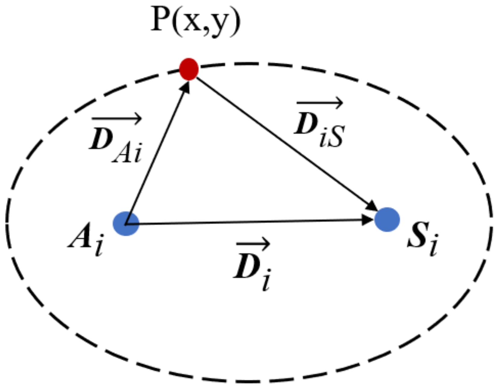
After the damage index values of all sensor paths are calculated, the second step of this algorithm is image reconstruction. The shape factor
can measure the size of the elliptical distribution, which is usually greater than 1.0 [
24]. The spatial distribution function
is expressed as [
17]:
where (
) are the coordinates of each point in a sensor array.
As shown in
Figure 1,
is the ratio of the sum of
and
to the distance between transmitter–receiver pairs
, which is expressed as [
17]:
Finally,
is defined as the damage characteristic parameters at each pixel, which represents the value of SDC, RMSE,
E1,
E2,
E3 and NCM. So, the damage probability of each point (
) of the detected area is calculated as follows [
17]:
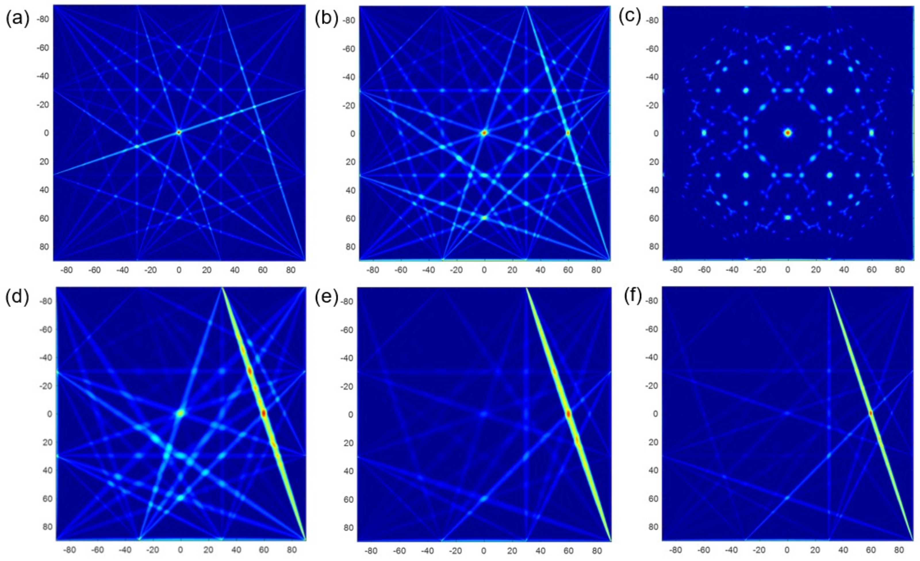
In the following study, we try to characterize the behavior of SDC, RMSE, E1, E2, E3 and NCM on monitoring pitting corrosion with the RAPID algorithm. In addition, in this work, we tried to distinguish a clear cognition to the effect of various corrosion damage characteristic parameters on image reconstruction so as to determine the best monitoring method.
2.2. Sensor Path Weighting RAPID Algorithm
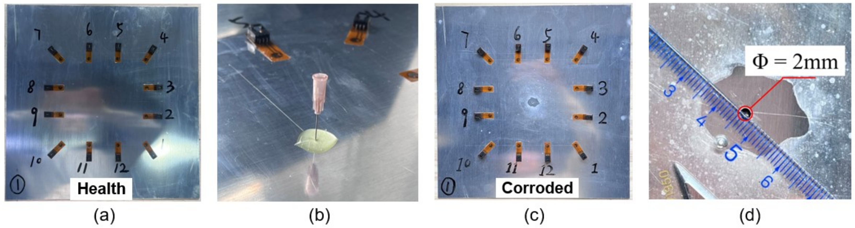
Generally speaking, the S0 mode and A0 mode have a similar effect on identifying multiple structural damage. However, the size of pitting corrosion in this paper is too tiny, and corrosion damage leads to the change of aluminum plate thickness. As we know, the Lamb wave A0 mode is sensitive to thickness variations, which is superior to that of S0 mode [
25]. Another essential property is that the A0 mode outperforms the S0 mode with a shorter wavelength and larger signal magnitude at relatively low frequencies (such as 110 kHz), which is beneficial to detect tiny damage [
26]. So, the A0 mode is selected to detect the signal differences caused by pitting corrosion.
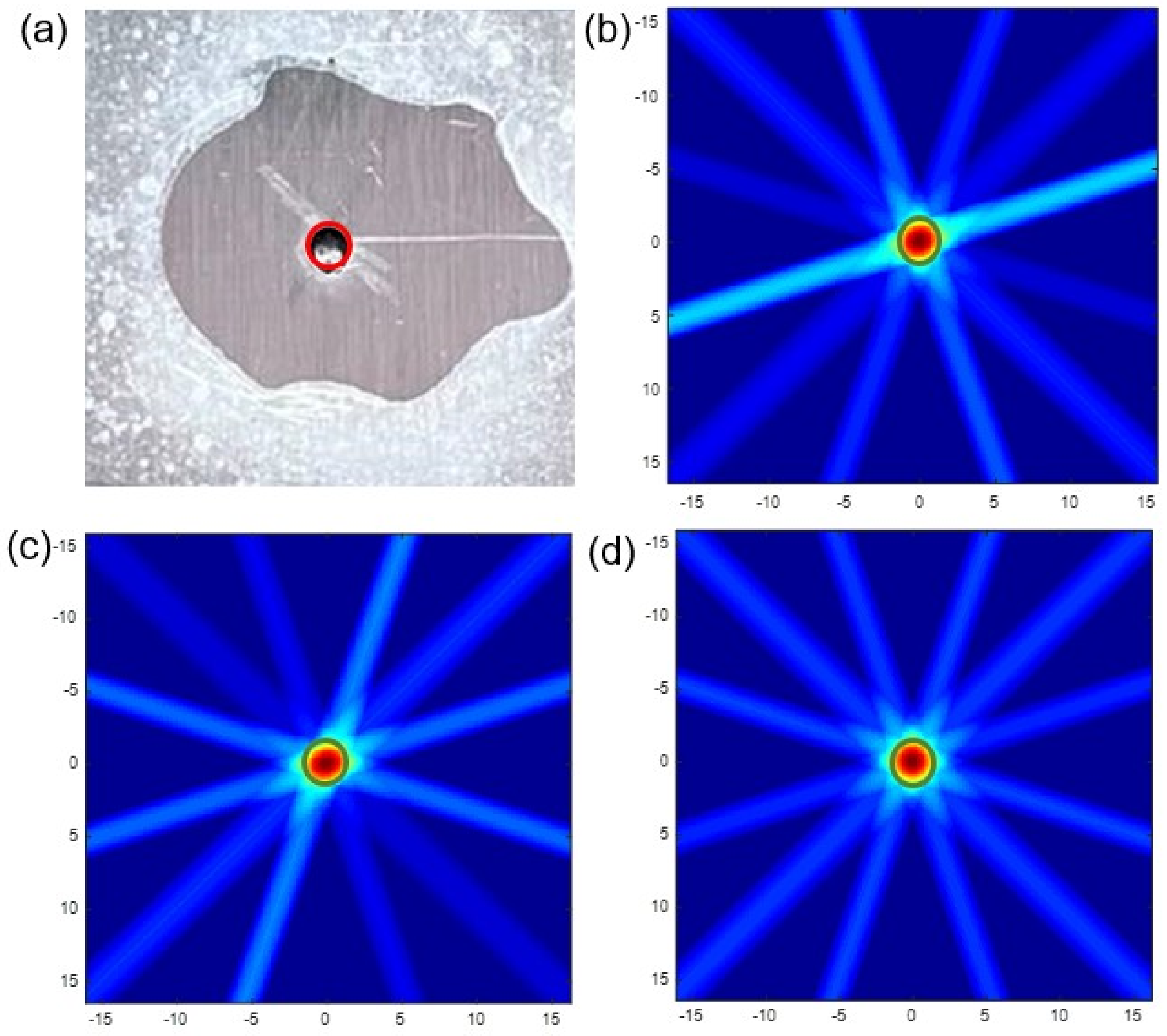
In the process of extracting damage feature information from the signal, two considerable factors are used to study the effect on the results, and both of them are related to the status of the sensor path. The first factor is whether the sensor path directly passes through the corrosion damage. Because when encountering damage, the ultrasonic signals will obtain different waves, such as reflected waves, diffracted waves, energy-attenuated waves and mode-converted waves [
27]. Subsequently, the amplitude and phase of signals are changed. So, it finally can represent whether a Lamb wave propagating on the sensor path carries effective damage feature information or not. On those paths not directly crossing through the corrosion part, the damage cannot interact with signals, which has a subtle effect on the A0 mode. Simultaneously, with the increase of the distance between sensor path and corrosion damage, the impact of damage on A0 mode gradually decreases. Therefore, the linear distance from sensor paths to pitting corrosion is established as
, which can evaluate how sensor paths are affected by corrosion damage.
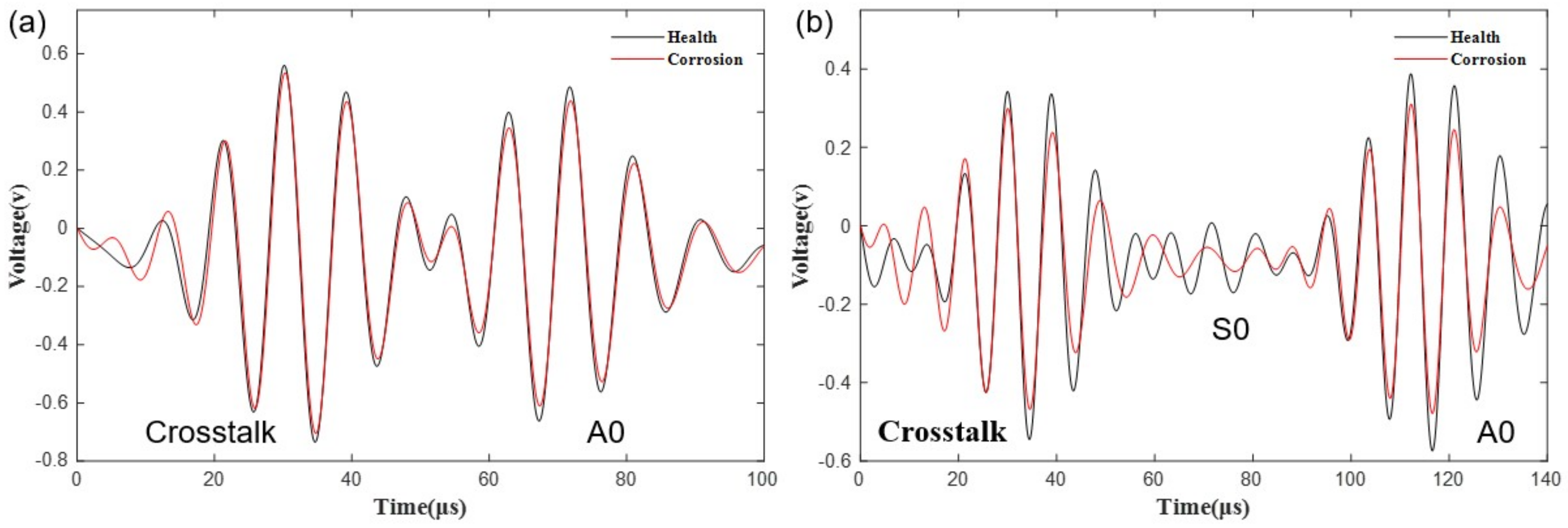
The second factor is the length of sensor path, which means the distance between sensor pairs. As expected, if sensor paths meet the condition that different Lamb wave modes can separate completely, it is convenient to obtain the damage feature information in signals. On the contrary, short sensor paths cannot provide sufficient propagation distance for signals, so the crosstalk in front, S0 mode and A0 mode will overlap with each other, making it difficult to obtain the important part of scattered signals [
28]. However, the existing RAPID algorithm does not take into account these two factors. Based on this problem, the algorithm needs to be modified.
The sensor path weighting RAPID (SPW-RAPID) algorithm is proposed on the basis of the RAPID algorithm. The sensor path weight from the transmitter
i and receiver
j sensor pair is established as
, which can modify and optimize the values of corrosion damage characteristic parameters. In addition, the value coefficient of sensor path from transmitter
i to receiver
j is proposed as
, which can describe how the sensor path is affected by pitting corrosion based on the first factor. The impact factor of the sensor path from the transmitter
i to receiver
j is put forward as
, which can evaluate the behavior of sensor path length to pitting corrosion identification based on the second factor. Finally, the sensor path is given a certain weight, which is defined as the product of value coefficient and impact factor on each sensor path, which is expressed as follows:
where
i represents the excitation sensor, and
j represents the receiving sensor.
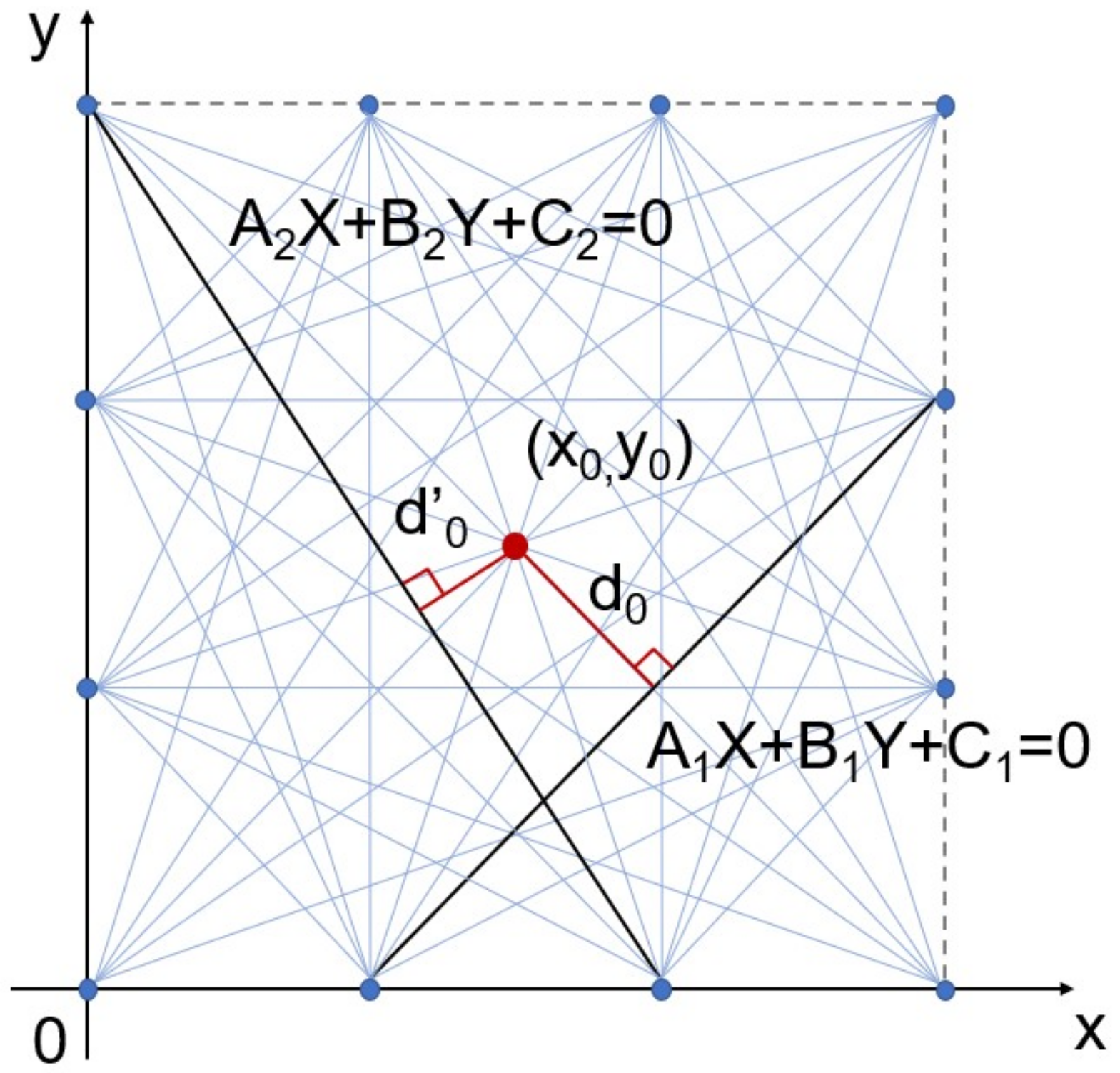
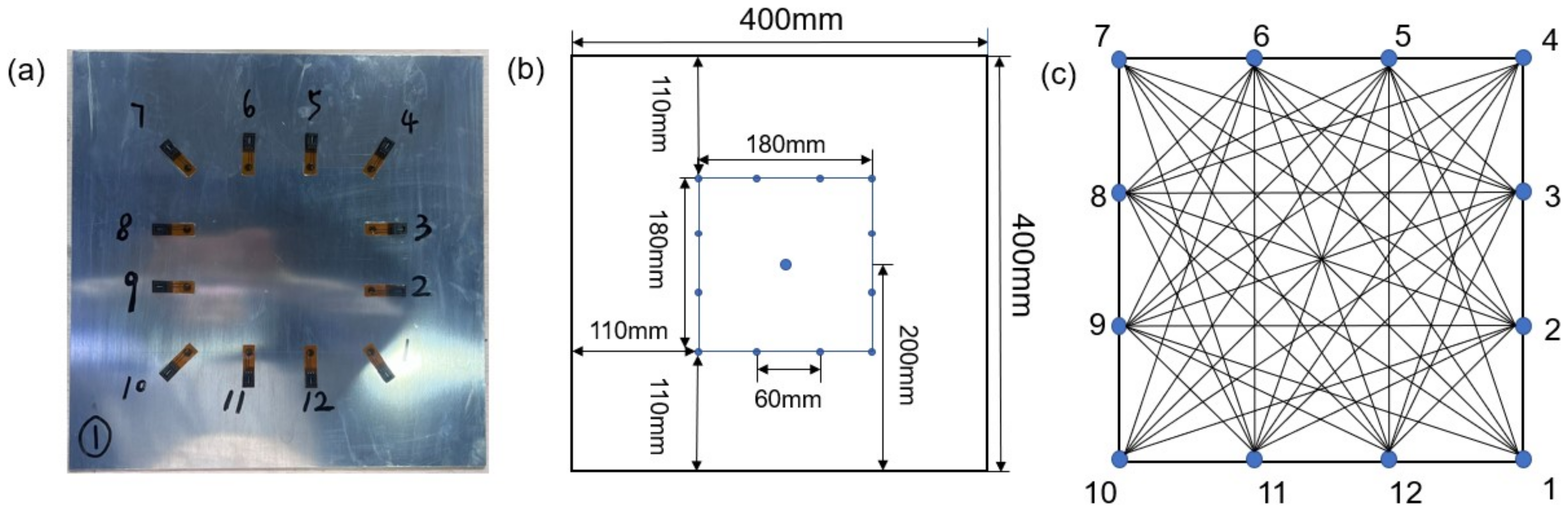
First of all, the value coefficient
needs to be determined. As we know, the traditional RAPID algorithm can roughly locate the pitting corrosion in the detected area and obtain the original pitting location
. A rectangular coordinate system is established based on the sensor network. Then, the linear expression of each sensor path in the coordinate can be obtained. According to the original pitting corrosion location
, the perpendicular distance from pitting corrosion to any sensor path can be calculated, as shown below:
where
A,
B and
C represent the coefficients of the linear equation in a rectangular coordinate system,
represents the horizontal ordinate of pitting position, and
represents the longitudinal ordinate of the pitting position.
Secondly, the sensor path value is established as
f, which describes the value level of sensor paths according to
and finally defines the
. The range of
is 0 to 1, where 1 represents the highest value and 0 represents no value. For instance, when
is equal to 0, the sensor path directly passes through the damage, where the signals can carry the most useful damage feature information, so its value is very high and
can be assigned as 1. With the increase of
, the damage is gradually away from the path. So, the damage feature information carried by signals reduces correspondingly, which devalues the sensor path and decreases the value of
. Additionally, those paths with a value coefficient of 0 are mostly located at the boundary of the sensor network. There is little important damage feature information in signals on the boundary path, which are vulnerable to plate edge reflection [
29].
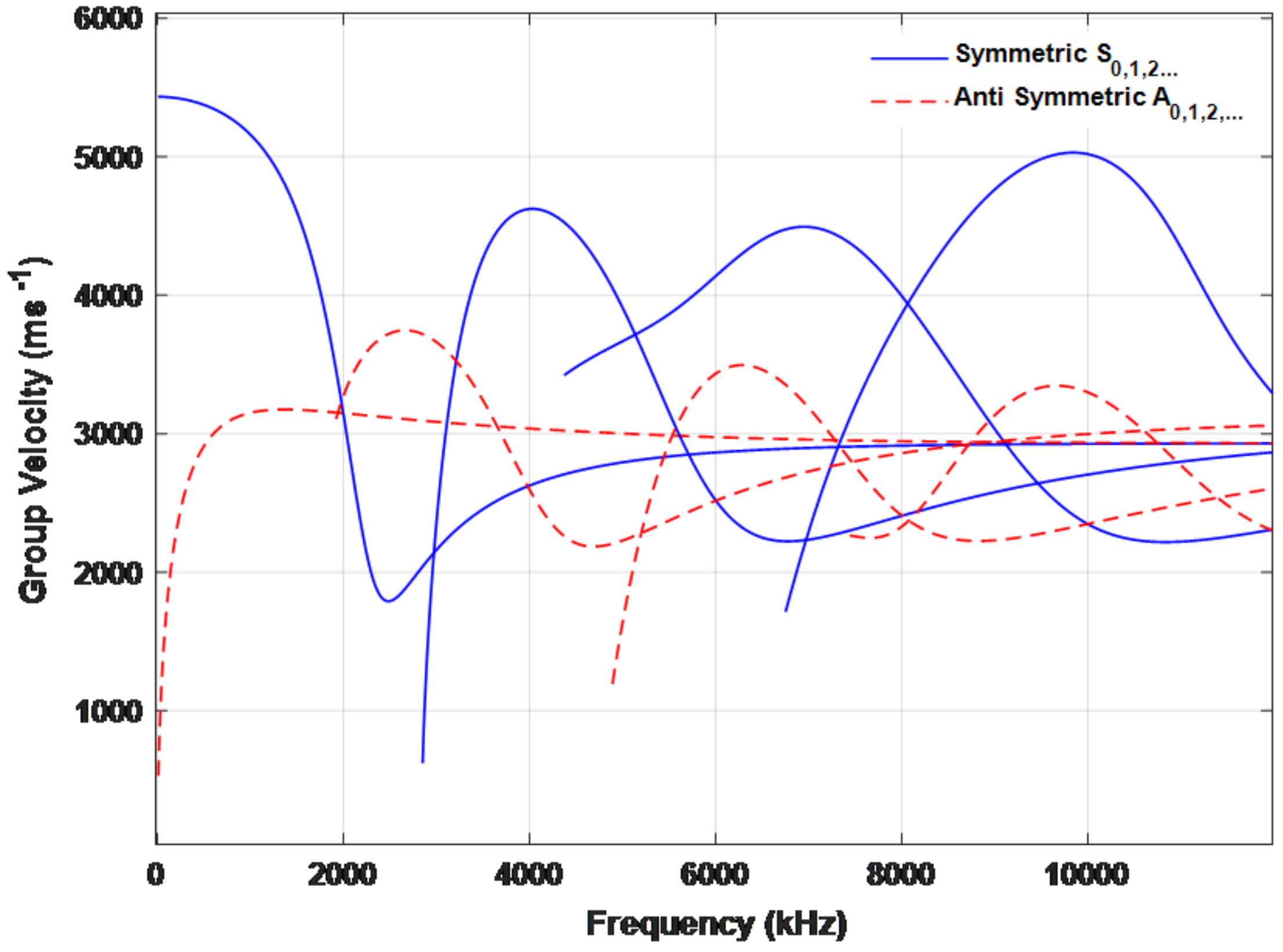
The third step is to determine the impact factor, whose range is 0 to 1 as well, and 1 represents that the influence of sensor path is great. Instead, 0 represents that there is no influence, because it is necessary to set a certain distance between sensors in order to extract an integral A0 mode. The distance between sensor pairs needs to satisfy as follows [
30]:
where
,
is the group velocity of the A0 mode and S0 mode, respectively;
is the central frequency of the excitation signal;
n indicates the number of cycles of the excitation signal;
L is the distance between sensor pairs.
The
from transmitter
i to receiver
j is expressed as:
Finally, the weight on each sensor path and the original corrosion damage characteristic parameters are multiplied to obtain the new corrosion damage characteristic parameters. The spatial distribution function and the damage probability are calculated as usual.
In order to evaluate the quality of imaging results, the accuracy and precision are put forward. Accuracy is the degree of closeness of barycentric coordinates between real damage and predicted damage. Distance Root Mean Squared (DRMS) is a good indicator to measure the distance between two points, as shown in Equation (
16). The bigger the DRMS value is, the larger the localization error is. Meanwhile, precision is the degree of imaging clarity, which can be obtained by enlarging the images for comparison.
where
represents the deviation of horizontal ordinate between real damage and predicted damage in a sensor network, and
represents the deviation of longitudinal ordinate between real damage and predicted damage in a sensor network.


