FADIT: Fast Document Image Thresholding


1
Northwest Institute of Eco-Environment and Resources, Chinese Academy of Sciences, Lanzhou 730000, China
2
National Cryosphere Desert Data Center, Lanzhou 730000, China
3
University of Chinese Academy of Sciences, Beijing 100049, China
*
Author to whom correspondence should be addressed.
Algorithms 2020, 13(2), 46; https://doi.org/10.3390/a13020046
Submission received: 8 February 2020
/
Revised: 18 February 2020
/
Accepted: 20 February 2020
/
Published: 21 February 2020
Abstract
:We propose a fast document image thresholding method (FADIT) and evaluations of the two classic methods for demonstrating the effectiveness of FADIT. We put forward two assumptions: (1) the probability of the occurrence of grayscale text and background is ideally two constants, and (2) a pixel with a low grayscale has a high probability of being classified as text and a pixel with a high grayscale has a high probability of being classified as background. With the two assumptions, a new criterion function is applied to document image thresholding in the Bayesian framework. The effectiveness of the method has been borne of a quantitative metric as well as qualitative comparisons with the state-of-the-art methods.
1. Introduction
Document image analysis (DIA) is an important area of pattern recognition [1]. Degraded document image restoration has become active research topic [2,3,4]. Restoration is difficult for document images suffering from various degradations such as faded ink, bleed-through, folding marks, show-through, uneven illumination, etc.
Image thresholding can be applied to the preprocessing of document image restoration because of its simplicity of implementation and relatively constant contrast of document images [5]. The role of thresholding is to remove the background as much as possible without modifying the text. Two of the most popular techniques for this purpose are Otsu’s method [6] and Kittler et al.’s method [7]. The comparison study of image thresholding obtains a conclusion that Kittler et al.’s method gives a better performance than others [8]. Kittler et al.’s optimum threshold is achieved by a criterion function related to average Bayesian classification error probability. Otsu’s method is the other thresholding that produces relatively good results [9,10]. Otsu’s threshold is determined by maximizing a discriminant function, but it tends to split the larger part when the sizes of object and background are unequal [11]. These well-known global thresholding methods have been widely applied to document image analysis [12,13,14,15,16].
Besides these global thresholding techniques, there are many local thresholding methods. Local thresholding is handled by applying different thresholds in different spatial regions. Sauvola et al. propose a sliding window-based method for document image thresholding [17]. Sauvola et al.’s method has a good performance [8], but has a high computational cost. A grid-based adaptive method is proposed to speed up Sauvola et al.’s [18]. With the grid-based technique, spatial discontinuity in the local gray-level information can be avoided by interpolation over the entire image to yield a smooth surface. With the grid-based technique, the performance of Saulova et al.’s is greatly improved [18]. The performance of these local thresholding methods depends heavily on the window or grid size and hence the character stroke width.
This paper presents a new thresholding technique called fast document image thresholding (FADIT) that selects the threshold by using a new criterion function under two assumptions. The two assumptions are proposed by using the relation and properties of text and background of document images to improve the performance of thresholding. When a threshold is determined by a classifier, the pixels with lower grayscales than the threshold are classified into text and the others are background, so we assume that (1) both of the text and background are uniform with constant probabilities and (2) pixels with lower grayscales have a larger probability to be classified as text and pixels with higher grayscales have a larger probability to be classified as background.
FADIT has been compared and benchmarked against classic methods and has shown better levels of efficiency and performance. Besides FADIT is compared with the two classic methods in this paper, we also conduct experiments to compare the FADIT with some state-of-the-art methods. Additionally, we apply the grid-based technique to FADIT and realize a grid-based FADIT scheme. The comparisons indicate the efficiency of FADIT and the grid-based FADIT by using two performance measures. Experimental results show that FADIT achieves a better performance than others in terms of visual quality and quantitative evaluations.
2. FADIT
2.1. Bayesian Framework
Suppose that the grayscale of an image is defined in the range , and the grayscale value is denoted by n. If an image is classified by the threshold into two classes that denote as and , the probability of occurrence of each grayscale n in the image is given by,
For a given grayscale n, is a constant that is determined by an image, the actual conditional probabilities and are able to be obtained after the threshold is determined, and and are easily to be calculated after the threshold is determined too.
Kittler et al. [7] assumed that each of the two components and is normally distributed. If the assumed and are substituted into Equation (1), the equation returns a new probability which is no longer equal to the actual . is related to the threshold , but is a constant that is determined by the image. As finding the optimized with respect to minimizing the Bayesian classification error probability is equivalent to maximizing correct classification probability, [7] adopt the average correct performance as the criterion function [7,19],
Kittler et al.’s method is not only in consideration of the Bayes minimum error probability, but also trying to approximate the actual through , which means that the maximum of the function Equation (2) over the threshold has the other explanation that is the maximum correlation of and ,
where the column vector is , and the column vector is .
We see from the first line in Equation (2) that is the mathematical expectation of the correct classification probability. With Bayes’ theorem [20], the posterior probabilities take the form of
Thus, the criterion function Equation (2) can be written also as
In next section, we propose two assumptions for the probability and the posterior probabilities and to obtain a new simple criterion function.
2.2. Criterion Function
Suppose that we select a threshold , and use it to threshold the document image into two classes, i and j, where i consists of all the pixels with grayscales in the range of and j consists of the pixels with grayscales in the range of . The black dark text belongs to class i and the white bright background belongs to class j in a document image. In this paper, we propose two assumptions for document images:
- Because both the dark text and the bright background are uniform in an ideal document image, we assume the probabilities of grayscales of the text and the background are two constants and respectively and the probabilities of other grayscales are 0. It means that once an image is segmented with threshold the image only have pure text and background. Under this assumption, a degraded document image is easily to be restored because Equation (3) implies that the actual probability tries to approximate the probability of the ideal document image. As Equation (2) is obtained by the maximum correct classification probability, and are given by the cumulative sum,The probabilities satisfy the constraint,
- A lower threshold makes its text pixels with lower grayscales, and a lower grayscale has larger posterior probability to be classified into text. The lower grayscale a pixel has, the larger probability it is classified into dark text, and the higher grayscale a pixel has, the larger probability it is classified into bright background, so we assume that the posterior probability of the dark text is a decreasing function of the threshold and the posterior probability of the bright background is an increasing function . The probabilities satisfy the constraint,
Based on the two assumptions, a new criterion function is given by,
which is obtained by substituting , and into Equation (6). Most values of are 0 except and , and we use and instead of and , respectively.
2.3. Posterior Probability Function
Generally, there are two facts in a document image:
- The mean of an image can be used to measure the average intensity of the image, and the average intensity of a document image mainly related with the bright background.
- If a document image is degraded, the text is still dark but the background tends to become tarnished. The background of a degraded document image is not very bright.
Based on the two facts, posterior probabilities functions and need to have the properties as the curves shown in Figure 1. We use the decreasing function of the following form,
where is the mean of the image.
The increasing function has the form of,
After a number of tests, is given by
The function decreases fast and the function increases fast too. Given two degraded document images with different mean, the intensity of background in the larger-mean image is larger than the smaller, so a pixel with high intensity in the smaller-mean image is more probable to be classified into background than the same gray value in the larger-mean image. For a pixel with a high intensity, the curve of corresponding to a smaller-mean image (right side of curve B) should always be above on the curve of corresponding to a larger-mean image (right side of curve D). According to Equation (10), the curves of have the opposite relationship. Consequently, the crossing point of and increases with increasing.
2.4. Speed-up Algorithms
Suppose that an image is denoted by I, and its grayscale variable is n. is the optimization variable and the optimal value is obtained by a criterion function.
The image histogram and the total pixel number N are computed by using the image to obtain the probability of occurrence of each grayscale n,
The global mean of the image is calculated by,
Using the threshold , , that the text assigned to class i is given by Equation (7). The background assigned to class j is given by,
The criterion function is computed easily and finding its maximum is a simple algorithm as shown in Algorithm 1.
| Algorithm 1: The FADIT algorithm. | |
| 1: | Compute the criterion function, , |
| 2: | for to do |
| 3: | , |
| 4: | , |
| 5: | , |
| 6: | end for |
| 7: | Obtain the FADIT threshold, . |
Otsu’s method [6] selects the threshold that maximizes the between-class variance defined as
where and are the means of grayscale of the pixels assigned to class i and class j, respectively.
The between-class variance has been rewritten to obtain fast algorithm [21] as,
where is the cumulative mean grayscale up to threshold and it is given by,
Thus, the fast Otsu’s algorithm is given by Algorithm 2.
| Algorithm 2: The fast Otsu’s algorithm. | |
| 1: | Compute the between-class variance, , |
| 2: | for to do |
| 3: | , |
| 4: | , |
| 5: | , |
| 6: | end for |
| 7: | Obtain the Otsu’s threshold, |
The criterion function of Kittler et al.’s method is given by [7],
where and are the variances of grayscale of the pixels assigned to class i and class j, respectively.
The variances and are calculated by,
Before using Equations (22) and (23) to obtain the criterion function, and are calculated by,
where is similar to Equation (20) and is calculated by,
Thus, the Kittler et al.’s algorithm is given by Algorithm 3.
The effectiveness of a thresholding algorithm depends strongly on the statistical characteristics of the image, and FADIT only use the probability rather than the mean and variance as shown in Table 1.
| Algorithm 3: The Kittler et al.’s algorithm. | |
| 1: | Compute the criterion function, , |
| 2: | for to do |
| 3: | , |
| 4: | , |
| 5: | , |
| 6: | , |
| 7: | , |
| 8: | , |
| 9: | , |
| 10: | , |
| 11: | |
| 12: | |
| 13: | end for |
| 14: | Obtain the Kittler et al.’s threshold, . |
3. Grid-Based FADIT
As the sliding window-based method has a high computational complexity and the block-based method has the block effect, the grid-based method is a compromise between window-based and block-based method. The grid-based method can greatly improve the performance of original Sauvola et al.’s method [18].
A parameter of the grid-based method, scale s, is suggested to be set to an odd number [18], and the grid step is set to . The grid step means that number of pixels are overlap between a grid and one of its neighboring grid.
The threshold in each sliding grid is calculated and stored into a matrix. The threshold matrix is interpolated by a differential calculus approach to yield a smooth surface [18,22]. The details of the grid-based implementation have been given in Moghaddam et al.’s paper [18] and the code can be found at the website of Mathworks (http://www.mathworks.com/matlabcentral/fileexchange/27808).
We obtain each threshold in each sliding grid by Algorithm 1, and the threshold matrix is interpolated to the size of input image. By the same way, Kittler et al.’s algorithm can use the grid-based technique too.
4. Experimental Results
The first experiment is conducted to demonstrate that FADIT method achieves performance of the classic methods (see Section 4.2).
The second experiment is conducted to demonstrate that the grid-based FADIT scheme achieves the state-of-the-art thresholding performance (see Section 4.3).
4.1. Experimental Setup
The effectiveness of FADIT has been tested with several images (see the first column of Figure 2) from dataset DIBCO. These images suffer from different degradation, which makes the thresholding a difficult work. The dataset also comprises their corresponding ground-truth images (see the last column of Figure 2), which are used to qualitatively compare the results of different methods.
We use peak signal-to-noise ratio (PSNR) and misclassification error (ME) [23] to quantitatively evaluate different algorithms. Larger PSNR indicates that the test image is more similar to the original (ground-truth) image. The ME varies from 0 for a perfectly classified image to 1 for a totally wrongly binarized image [8].
For the two-class segmentation problem, ME can be expressed as:
where and denote the background and foreground of the original (ground-truth) image, and denote the background and foreground area pixels in the test image, and is the cardinality of the set •.
4.2. FADIT Compared with Classic Algorithms
In this section, experiments are conducted to demonstrate the effectiveness of FADIA by comparing FADIT method with two classic thresholding methods: Otsu’s method and Kittler et al.’s method, and the experimental results are shown in Figure 2.
In Otsu’s method, the between-class variance can also be written as,
The criterion function Equation (28) maximizes both the term and the term simultaneously. The term produces the maximum value when the object and background has same pixels. The other term determines the criterion function to be similar to the liner discriminant analysis. Although Otsu’s method is popular in image thresholding, it is not suitable for degraded document image. Kittler et al.’s method selects the global threshold corresponding to minimum thresholding error based on the assumption that each class is normally distributed, which limits its application because local regions do not always obey a normal distribution. FADIT method is based on two reasonable assumptions directly according to the inherent characteristics of degraded document image, so it obtains good thresholding results.
For image 1, the result of FADIT remains the least shadow in the right side and the difference can be easily seen in Figure 2b–d, so our result displays all the characters. After the comparison of the results of image 2, image 4 and image 5, we find that: (1) results of Otsu’s method render the handwriting thin and even discontinuous, (2) results of Kittler et al.’s method has many black points in the background, and (3) results of FADIT are quite close to the ground-truth images. Especially, the result of image 5 obtained by Kittler et al.’s method (see Figure 2w) preserves background texture and some characters of the back side. For image 3, Otsu’s and Kittler et al.’s methods produce the worst results (see Figure 2l,m), and in them dark blocks totally cover the text.
We quantitatively evaluate different methods with the five images and list the result in Table 2. For any image, FADIT method obtains the largest PSNR and the smallest ME, which means that the objective quantitative evaluation is consistent with the subjective visual effect of the thresholding results. Meanwhile, FADIT algorithm runs much faster than Otsu’s and Kittler et al.’s algorithm.
4.3. Grid-based FADIT Compared with Other Algorithms
The grid-based FADIT method is compared with Sauvola method [17], grid-based Sauvola method [18], and GLGM (gray-level and gradient-magnitude) histogram method [24]. We also present the results of grid-based Kittler et al.’s method. [18] obtain a conclusion that grid-based Sauvola et al.’s method is better than the grid-based Otsu’s method, so we do not show the grid-based Ostu method in this section.
In all of grid-based methods, is set to
where r and c denote numbers of row and column of the image, respectively.
The image results of the mentioned methods are in Figure 3. Different from Otsu’s, Kittler et al.’s or FADIT method, Sauvola method selects a threshold for each pixel, then obtains a thrshold matrix with the same size of the input image. Every threshold is calculated in the window centering on the corresponding pixel, so the algorithm runs quite slow, and the running time can been seen in Figure 3. From Figure 3a,f,k,p,u, we can see that the method can successfully extract the characters but can not obtain good result for the whole image as the background contains so much black noise. Moghaddam et al. [18] have demonstrated that the grid-based technique greatly improved the results of Sauvola et al.’s method, which can be seen from Figure 3b,g,l,q,v. As such, we apply grid-based technique into Kittler et al.’s and FADIT method. Figure 3 shows that grid-based technique indeed improves the results of Kittler et al.’s and FADIT method. However, grid-based Kittler et al.’s method still suffers from the problem in Figure 2m (see Figure 3m) while grid-based FADIT method obtains results all quite close to ground-truth images. GLGM method is a novel thresholding method which selects a global threshold based on the GLGM histogram, and it obtains satisfying results with natural images [24] while not with document images (see Figure 3x).
The quantitative evaluation result of different methods with the five images is listed in Table 3. According to the metrics, a grid-based FADIT method have outperformed the above methods.
5. Conclusions
Segmentation of text from degraded document images is a very challenging task. Experimentally, FADIT is compared against Otsu’s and Kittler et al.’s thresholding techniques. Although image thresholding has been popular in image segmentation for over 50 years, the classic Otsu’s and Kittler et al.’s methods still produce relatively better results than others [8]. FADIT obtains a better segment results than two classic methods and has a lower computational complexity. FADIT is a nonparametric technique to find the optimal threshold through the optimization of a new criterion function, and is a simple and robust algorithm for document image thresholding. Experimental results of FADIT can properly segment out text from background and they are quite close to the ground-truth images.
Since it does well in binary segmentation, FADIT can be applied to some specific applications, e.g., saliency detection. Most saliency detection tasks use a very clear object in an image and the image is captured by focusing the object in attention. FADIT can be used to produce a reference results for training a neural network in unsupervised way. Furthermore, FADIT can be used to generate pseudo labels for weakly labeled segmentation tasks. Since FADIT is good at segmenting binary targets and many medical image segmentation tasks only need to segment a specific organ, and medical images can be segmented by FADIT, at least it can obtain pseudo labels for training a neural networks.
Author Contributions
Y.M. did the experimental results and wrote the manuscript. Y.Z. discussed with Y.M. and gave many useful suggestions. All authors have read and agreed to the published version of the manuscript.
Funding
This work was supported by the 13th Five-year Informatization Plan of the Chinese Academy of Sciences, Grant Nos. XXH13506 and XXH13505-220, aAnd Data sharing fundamental program for Construction of the National Science and Technology Infrastructure Platform (Y719H71006). Technical support was provided by the National Cryosphere and Desert Scientific Data Center of China.
Conflicts of Interest
The authors declare no conflicts of interest.
References
- Nagy, G. Twenty years of document image analysis in PAMI. IEEE Trans. Pattern Anal. Mach. Intell. 2000, 22, 38–62. [Google Scholar] [CrossRef]
- Lelore, T.; Bouchara, F. FAIR: A Fast Algorithm for Document Image Restoration. IEEE Trans. Pattern Anal. Mach. Intell. 2013, 35, 2039–2048. [Google Scholar] [CrossRef] [PubMed] [Green Version]
- Rowley-Brooke, R.; Pitie, F.; Kokaram, A. A Non-parametric Framework for Document Bleed-through Removal. In Proceedings of the IEEE Conference on Computer Vision and Pattern Recognition (CVPR), Portland, OR, USA, 23–28 June 2013; pp. 2954–2960. [Google Scholar]
- Su, B.; Lu, S.; Tan, C.L. Robust document image binarization technique for degraded document images. IEEE Trans. Image Process. 2013, 22, 1408–1417. [Google Scholar] [PubMed]
- Solihin, Y.; Leedham, C. Integral ratio: A new class of global thresholding techniques for handwriting images. IEEE Trans. Pattern Anal. Mach. Intell. 1999, 21, 761–768. [Google Scholar] [CrossRef]
- Otsu, N. A threshold selection method from gray-level histograms. IEEE Trans. Syst. Man Cybern. 1979, SMC-9, 62–66. [Google Scholar] [CrossRef] [Green Version]
- Kittler, J.; Illingworth, J. Minimum error thresholding. Pattern Recognit. 1986, 19, 41–47. [Google Scholar] [CrossRef]
- Sezgin, M.; Sankur, B. Survey over image thresholding techniques and quantitative performance evaluation. J. Electron. Imaging 2004, 13, 146–168. [Google Scholar]
- Lee, S.U.; Chung, S.Y.; Park, R.H. A comparative performance study of several global thresholding techniques for segmentation. Comput. Vis. Graph. Image Process. 1990, 52, 171–190. [Google Scholar] [CrossRef]
- Trier, B.D.; Jain, A.K. Goal-directed evaluation of binarization methods. IEEE Trans. Pattern Anal. Mach. Intell. 1995, 17, 1191–1201. [Google Scholar] [CrossRef]
- Kittler, J.; Illingworth, J. On threshold selection using clustering criteria. IEEE Trans. Syst. Man Cybern. 1985, SMC-15, 652–655. [Google Scholar] [CrossRef]
- Cheriet, M.; Said, J.N.; Suen, C.Y. A recursive thresholding technique for image segmentation. IEEE Trans. Image Process. 1998, 7, 918–921. [Google Scholar] [CrossRef] [PubMed] [Green Version]
- Zhan, K.; Zhang, H.; Ma, Y. New spiking cortical model for invariant texture retrieval and image processing. IEEE Trans. Neural Netw. 2009, 20, 1980–1986. [Google Scholar] [CrossRef] [PubMed]
- Nina, O.; Morse, B.; Barrett, W. A recursive Otsu thresholding method for scanned document binarization. In Proceedings of the 2011 IEEE Workshop on Applications of Computer Vision (WACV), Kona, HI, USA, 5–7 January 2011; pp. 307–314. [Google Scholar]
- Moghaddam, R.F.; Cheriet, M. AdOtsu: An adaptive and parameterless generalization of Otsu’s method for document image binarization. Pattern Recognit. 2012, 45, 2419–2431. [Google Scholar] [CrossRef]
- Zhan, K.; Shi, J.; Li, Q.; Teng, J.; Wang, M. Image segmentation using fast linking SCM. In Proceedings of the 2015 International Joint Conference on Neural Networks (IJCNN), Killarney, Ireland, 12–17 July 2015; Volume 25, pp. 2093–2100. [Google Scholar]
- Sauvola, J.; Pietikäinen, M. Adaptive document image binarization. Pattern Recognit. 2000, 33, 225–236. [Google Scholar] [CrossRef] [Green Version]
- Moghaddam, R.F.; Cheriet, M. A multi-scale framework for adaptive binarization of degraded document images. Pattern Recognit. 2010, 43, 2186–2198. [Google Scholar] [CrossRef]
- Ye, Q.Z.; Danielsson, P.E. On minimum error thresholding and its implementations. Pattern Recognit. Lett. 1988, 7, 201–206. [Google Scholar] [CrossRef]
- Bishop, C.M. Pattern Recognition and Machine Learning; Springer Science Business Media: New York, NY, USA, 2006; pp. 21–24. [Google Scholar]
- Gonzalez, R.C.; Woods, R.E.; Eddins, S.L. Digital Image Processing Using MATLAB. Available online: https://www.mathworks.com/academia/books/digital-image-processing-using-matlab-gonzalez.html (accessed on 21 February 2020).
- Kerr, M.; Burrage, K. New Multivalue Methods for Differential Algebraic Equations. Numer. Algorithms 2002, 31, 193–213. [Google Scholar] [CrossRef]
- Yasnoff, W.A.; Mui, J.K.; Bacus, J.W. Error measures for scene segmentation. Pattern Recognit. 1977, 9, 217–231. [Google Scholar] [CrossRef]
- Xiao, Y.; Cao, Z.; Yuan, J. Entropic image thresholding based on GLGM histogram. Pattern Recognit. Lett. 2014, 40, 47–55. [Google Scholar] [CrossRef]
Figure 1.
Posterior probabilities functions and with different parameters .

Figure 2.
The input images are shown in the first column: (a) image 1, (f) image 2, (k) image 3, (p) image 4 and (u) image 5. The second (b,g,l,q,v), third (c,h,m,r,w), and forth (d,i,n,s,x) columns are results obtained by Otsu’s, Kittler et al.’s, and FADIT methods, respectively. Images in the last column (e,j,o,t,y) are the corresponding ground-truth images.
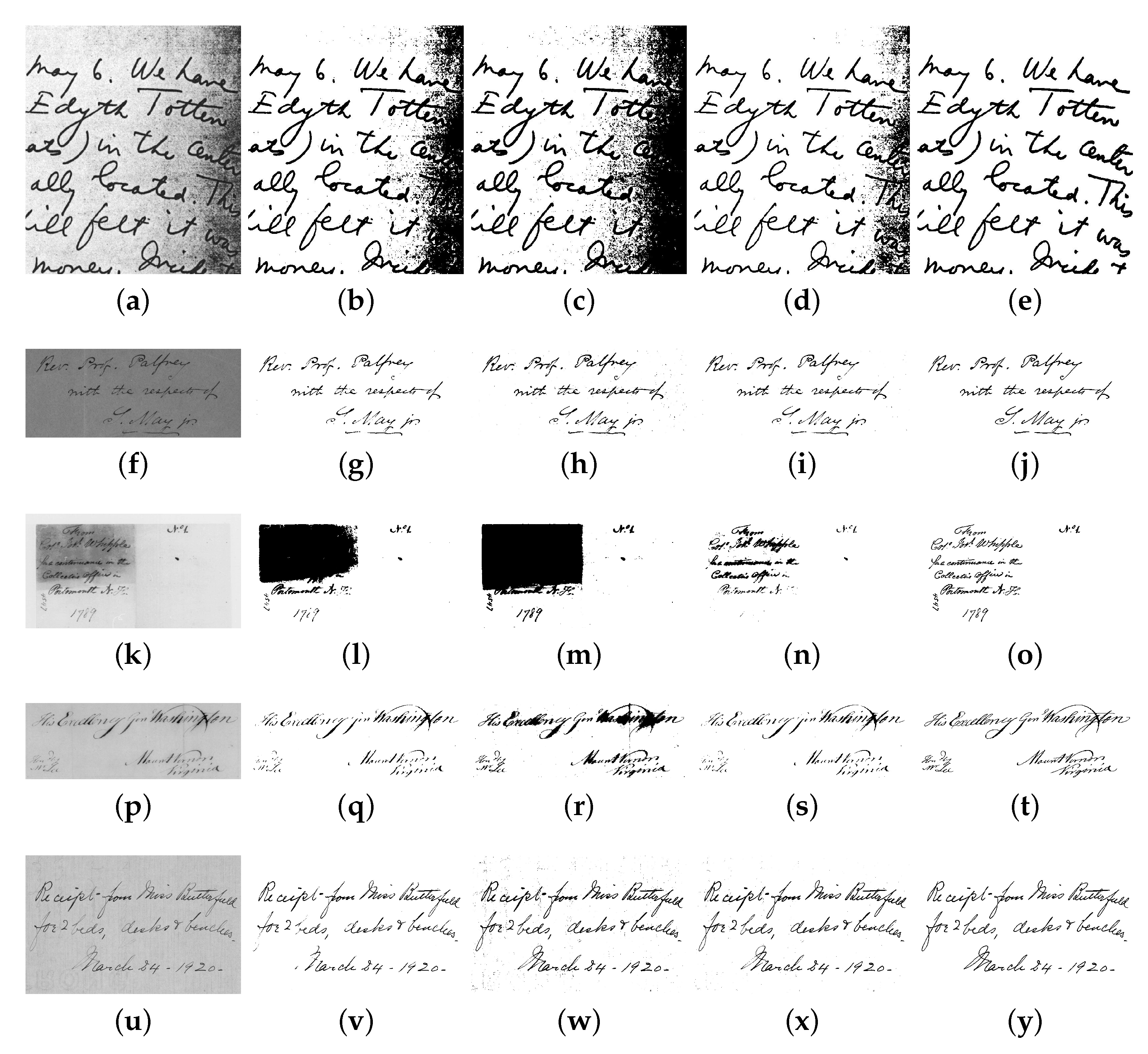
Figure 3.
Results obtained by different thresholding methods: Each column from left to right shows the results of Sauvola (a,f,k,p,u), Grid-based Sauvola et al.’s (b,g,l,q,v), Grid-based Kittler et al.’s (c,h,m,r,w), GLGM (d,i,n,s,x), and Grid-based FADIT method (e,j,o,t,y), respectively.
Figure 3.
Results obtained by different thresholding methods: Each column from left to right shows the results of Sauvola (a,f,k,p,u), Grid-based Sauvola et al.’s (b,g,l,q,v), Grid-based Kittler et al.’s (c,h,m,r,w), GLGM (d,i,n,s,x), and Grid-based FADIT method (e,j,o,t,y), respectively.


Table 1.
Comparison of FADIT, Otsu’s, Kitter et al.’s algorithms, “✓” denotes the corresponding item is necessary to be calculated while “×” denotes not.
Table 1.
Comparison of FADIT, Otsu’s, Kitter et al.’s algorithms, “✓” denotes the corresponding item is necessary to be calculated while “×” denotes not.
| FADIT | Otsu’s | Kitter et al.’s | |
|---|---|---|---|
| ✓ | ✓ | ✓ | |
| × | ✓ | ✓ | |
| × | × | ✓ | |
| × | × | × | |
| × | × | × | |
| × | × | ✓ |
Table 2.
Objective performance of different methods.
| Peak Signal-to-Noise Ratio (dB) | |||
| Otsu | Kittler | FADIT | |
| Image 1 | 9.2647 | 7.1802 | 11.5618 |
| Image 2 | 20.1543 | 20.3800 | 20.9538 |
| Image 3 | 7.2727 | 6.2408 | 16.0214 |
| Image 4 | 16.5733 | 13.1810 | 16.7075 |
| Image 5 | 20.3387 | 19.9889 | 21.5522 |
| Misclassification Error | |||
| Otsu | Kittler | FADIT | |
| Image 1 | 0.1184 | 0.1914 | 0.0698 |
| Image 2 | 0.0097 | 0.0092 | 0.0080 |
| Image 3 | 0.1874 | 0.2376 | 0.0250 |
| Image 4 | 0.0220 | 0.0481 | 0.0213 |
| Image 5 | 0.0092 | 0.0100 | 0.0070 |
| Running Time in MATLAB (Microsecond) | |||
| Otsu | Kittler | FADIT | |
| Image 1 | 2.5779 | 3.4130 | 1.6194 |
| Image 2 | 2.5601 | 3.3707 | 1.6029 |
| Image 3 | 2.5841 | 3.4544 | 1.6101 |
| Image 4 | 2.5750 | 3.4324 | 1.6071 |
| Image 5 | 2.5761 | 3.4037 | 1.6105 |
Table 3.
Objective performance of different methods.
| Peak Signal-To-Noise Ratio (dB) | |||||
| Sauvola | Grid-Sauvola | Grid-Kittler | GLGM | Grid-FADIT | |
| Image 1 | 7.3912 | 10.6198 | 8.1273 | 9.4828 | 13.0383 |
| Image 2 | 4.6402 | 16.4017 | 20.4056 | 19.9702 | 20.5779 |
| Image 3 | 3.6341 | 14.0252 | 6.2377 | 15.6426 | 17.6719 |
| Image 4 | 4.7587 | 14.4093 | 13.6244 | 14.0242 | 16.6563 |
| Image 5 | 4.7563 | 17.4495 | 20.0865 | 15.0982 | 21.5843 |
| Misclassification Error | |||||
| Sauvola | Grid-Sauvola | Grid-Kittler | GLGM | Grid-FADIT | |
| Image 1 | 0.1823 | 0.0867 | 0.1539 | 0.1126 | 0.0497 |
| Image 2 | 0.3435 | 0.0229 | 0.0091 | 0.0101 | 0.0088 |
| Image 3 | 0.4331 | 0.0396 | 0.2378 | 0.0273 | 0.0171 |
| Image 4 | 0.3343 | 0.0362 | 0.0434 | 0.0396 | 0.0216 |
| Image 5 | 0.3345 | 0.0180 | 0.0098 | 0.0309 | 0.0069 |
| Running Time in MATLAB (Second) | |||||
| Sauvola | Grid-Sauvola | Grid-Kittler | GLGM | Grid-FADIT | |
| Image 1 | 38.5553 | 3.7726 | 1.8631 | 0.7000 | 1.8401 |
| Image 2 | 32.3430 | 3.2322 | 1.6674 | 0.5537 | 1.5850 |
| Image 3 | 75.5198 | 7.4040 | 3.6795 | 1.3186 | 3.6751 |
| Image 4 | 87.3679 | 8.4955 | 4.2793 | 1.5257 | 4.2375 |
| Image 5 | 75.0670 | 7.3851 | 3.6802 | 1.3247 | 3.6703 |
© 2020 by the authors. Licensee MDPI, Basel, Switzerland. This article is an open access article distributed under the terms and conditions of the Creative Commons Attribution (CC BY) license (http://creativecommons.org/licenses/by/4.0/).
Share and Cite
MDPI and ACS Style
Min, Y.; Zhang, Y. FADIT: Fast Document Image Thresholding. Algorithms 2020, 13, 46. https://doi.org/10.3390/a13020046
AMA Style
Min Y, Zhang Y. FADIT: Fast Document Image Thresholding. Algorithms. 2020; 13(2):46. https://doi.org/10.3390/a13020046
Chicago/Turabian StyleMin, Yufang, and Yaonan Zhang. 2020. "FADIT: Fast Document Image Thresholding" Algorithms 13, no. 2: 46. https://doi.org/10.3390/a13020046
Note that from the first issue of 2016, this journal uses article numbers instead of page numbers. See further details here.