Linking Vegetation Diversity and Soils on Highway Slopes: A Case Study of the Zhengzhou–Xinxiang Section of the Beijing–Hong Kong–Macau Highway

Abstract

The rapid development of highways has caused a series of ecological problems, the restoration of which is an important part of highway construction. However, most related studies have focused only on the early stages of slope restoration. The present study investigated the Zhengzhou–Xinxiang section of the Beijing–Hong Kong–Macau Highway, which has been restored over more than 20 years, examining nine representative vegetation communities within this section and investigating their species diversity and soil physicochemical properties. Redundancy analysis and the grey correlation degree model were used to determine the relationship and coupling mechanism between vegetation diversity and soil physiochemical properties. The results showed some differences in the diversity of different vegetation communities and soil physicochemical properties; vegetation diversity was mainly influenced by organic material, total and available nitrogen, total and available phosphorus, slope, available potassium, and soil bulk density. Overall, environmental factors had a strong correlation with the Simpson dominance index and a weak correlation with the species richness index. The degree of coordination between vegetation community diversity and the soil coupling of the road slope remained on low and medium levels. Artificial vegetation restoration can regulate water and fertilizer resources and promote the restoration of highway slope vegetation.

1. Introduction

Highways form a broadly distributed network over the land, splitting and fragmenting the natural environment [1]. Thus, although highway construction brings huge economic benefits, it can also lead to a series of ecological problems. China’s highway construction is unique, usually with deep excavations and high fill levels along the sides, causing ecological damage along the route and directly or indirectly damaging the natural environment. These constructions form a large number of slopes with special fields, resulting in a sharp decline in the quality of the human environment, which greatly increases the expense of highway management [2,3,4,5]. Reconstruction and restoration of highway slope vegetation is the key and difficult point of highway ecological restoration, as well as an important measure for the protection of highway slopes. Highway slope vegetation restoration is mainly restricted by environmental factors such as terrain and soil, as soil is the material basis for plant growth, providing water and nutrients to vegetation communities and thus directly affecting plant growth. The presence of vegetation, particularly on slopes, reduces soil erosion and plays an important role in the restoration of target plant assemblages on slopes adjacent to highways [6,7]. In the process of vegetation restoration, changes in vegetation community and soil nutrient characteristics interact with each other [8,9,10,11,12]. As the mechanism of vegetation–soil interaction is complex, these effects can be positive or negative [13]. Therefore, vegetation communities and soils are the focus of research on the ecological restoration of slopes, and studying the relationship between them can provide theoretical guidance for future artificial intervention [14].

However, most studies have focused on the early stages of highway slope restoration [15,16], and relevant research on highway slopes that have been in the restoration process for more than 20 years is lacking. The target vegetation, vegetation community structure, and dominant species planned in the early stages of restoration changed significantly, and the coupling relationship between the vegetation community and soil is not clear. Therefore, the present study examined the slope of the Zhengzhou–Xinxiang section of the Beijing–Hong Kong–Macau Highway, which has been planted as part of its restoration for 24 years. We examined nine representative vegetation communities within this section and investigated their species diversity and soil physicochemical properties. Redundancy analysis (RDA) and the grey correlation degree model were used to determine the relationship and coupling mechanism between vegetation diversity and soil physiochemical properties. The purpose of this study was to address the following objectives: (1) to analyze the characteristics of species diversity and soil physicochemical properties in different vegetation communities; (2) to clarify the relationship between the environmental factors and species diversity of these vegetation communities; (3) to analyze the coupling between the species diversity and environmental factors in different vegetation communities. We hypothesize that (1) the indicators of species diversity and environmental factors of vegetation communities differ significantly; (2) the main factors affecting species diversity of vegetation communities can be distinguished; and (3) the coupling degree between species diversity and environmental factors of different vegetation communities can be clarified. Ultimately, we aim to provide scientific basis for vegetation community management, selection, as well as species diversity protection in the process of highway slope ecological restoration and reconstruction.

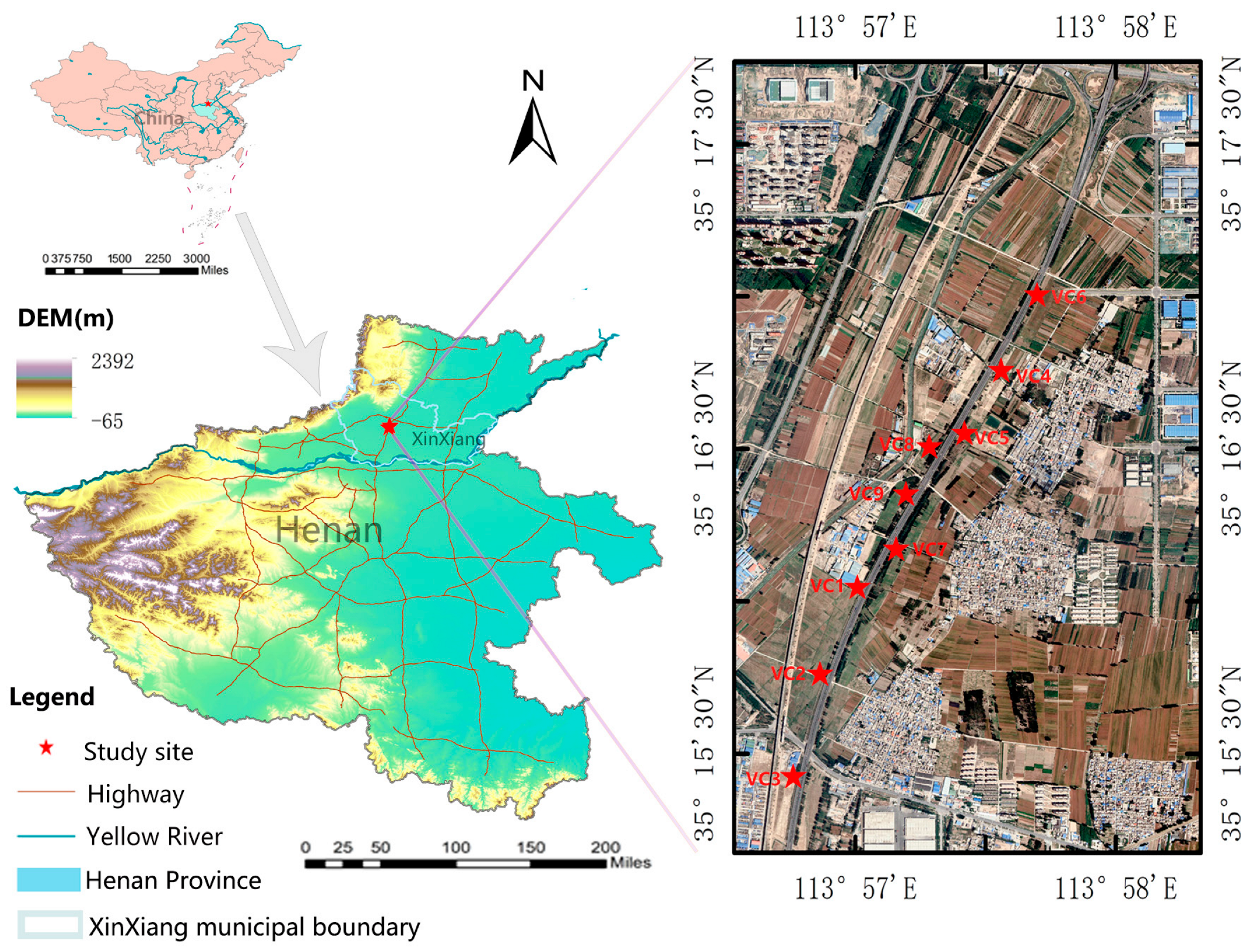
2. General Characteristics of the Study Area

The Beijing–Hong Kong–Macau Highway extends from Liuliqiao on the Third Ring Road in the southwest of Beijing in the north, passing through Hebei, Henan, Hubei, and Hunan. It is divided into two parts in Guangdong, leading to Hong Kong and Macau, with a total length of about 2285 km. It is one of China’s major north–south transportation arteries. The Henan section of the Beijing–Hong Kong–Macau Highway passes through Anyang, Hebi, Xinxiang, Zhengzhou, Xuchang, Luohe, Zhumadian, and Xinyang. As shown in Figure 1, the Zhengzhou–Xinxiang section was selected as the study area, with a total of 38 km of general survey coverage. After 24 years of vegetation restoration, we found that the study section has a large number of trees such as Broussonetia payrifera (Linn.) L’Hér. ex Vent. and Ulmus pumila L. as well as a small number of Melia azedarach, Populus tomentosa, and Styphnolobium japonicum (L.). The tree community was mainly concentrated in the Xinxiang section. The community structure type changed from shrub to trees + shrubs + grasses, shrubs + grasses, and trees + grasses. The early vegetation on the slopes of the studied highway was the native species Amorpha fruticosa L., with a planting density of 2–4 plants per meter. This section was opened to traffic in November 1997 and is located in Xinxiang City, which has a northern temperate continental climate with four distinct seasons: cold winter, hot summer, cool autumn, and early spring. The highest temperature is 42.7 °C, the lowest temperature is −21.3 °C, and the average annual temperature is 14 °C. July is the hottest month with an average temperature of 27.3 °C, and January is the coldest month with an average temperature of 0.2 °C. The average annual precipitation is 573.4 mm.

3. Materials and Methods

3.1. Vegetation Community Research

In October 2021, vegetation of the Zhengzhou–Xinxiang section of the Beijing–Hong Kong–Macau Highway was investigated. The main vegetation communities were the A. fruticosa, B. papyrifera, and U. pumila communities, among which the B. papyrifera and U. pumila communities were mostly concentrated in the Xinxiang section. Nine representative vegetation communities were selected, as shown in

Table 1. Names of vegetation communities in the study section and basic information regarding the sample plots.

VC	Name of Vegetation Community	Slope	Orientation
VC1	Guandi B. papyrifera	32°	West Slope
VC2	Guandi U. pumila + A. fruticosa	46°	West Slope
VC3	Guandi A. fruticosa + Artemisia annua	46°	West Slope
VC4	Zhangdi B. papyrifera + A. fruticosa	31°	East Slope
VC5	Zhangdi U. pumila + A. fruticosa	31°	East Slope
VC6	Zhangdi A. fruticosa	35°	East Slope
VC7	Yuandi B. papyrifera	30°	East Slope
VC8	Yuandi Humulus scandens + B. papyrifera	31°	West Slope
VC9	Yuandi Setaria viridis (L.) Beauv. + A. fruticosa	31°	West Slope

VC is short for vegetation community (the same below). Guandi, Zhangdi, and Yuandi are place names.

. The community structure included trees + shrubs + grasses, shrubs + grasses, and trees + grasses, and the communities were named according to the geographical location and dominant species. As shown in Figure 2, because the slope of the study section was protected by an arched skeleton, each sample plot was constructed with upper, middle, and lower three-arch frames (4 m × 10 m). The sampling of each vegetation community was repeated three times, with a total of 27 sample plots. For each tree species, the breast-height diameter, tree height, crown width, and number of trees were recorded. For the shrub species, species names, the height, crown width, and number of shrubs in each sample plot were determined. Three 1 m × 1 m quadrats were established along the diagonal of each sample plot, with a total of 81 quadrats. These quadrats were used to record the type, height, coverage, and number of herbaceous plant stands.

3.2. Determination of Vegetation Community Diversity

Species diversity can reflect the community structure and characteristics. The present study focused on α-diversity, and the selected indices included the species richness index (R), Shannon–Wiener diversity index (H), Pielou’s evenness index (E), and Simpson dominance index (D). The calculation methods were as follows [17,18]:

Richness index (R): number of vegetation species in a sample plot or quadrat.

$$\mathrm{R}=\mathrm{S}$$

(1)

The Shannon–Wiener diversity index (H) was calculated as:

$$\mathrm{H}=-{\sum }_{\mathrm{i}=1}^{\mathrm{S}}\left({\mathrm{P}}_{\mathrm{i}}\ln {\mathrm{P}}_{\mathrm{i}}\right) {{\mathrm{P}}_{\mathrm{i}}=\mathrm{N}}_{\mathrm{i}}/\mathrm{N}$$

(2)

Pielou’s evenness index (E) was calculated as:

$$\mathrm{E}=\mathrm{H}/\mathrm{l}\mathrm{n}\mathrm{S}$$

(3)

The Simpson dominance index (D) was calculated as:

$$\mathrm{D}=1-{\sum }_{\mathrm{i}=1}^{\mathrm{s}}{\mathrm{P}\mathrm{i}}^2$$

(4)

In the above equations, S denotes the number of species in the sample plot, N denotes the number of individuals of all species in the sample plot, Ni denotes the number of individuals of the i-th species in the sample plot, and Pi is the density of the i-th species in the sample plot.

3.3. Determination of Soil Physicochemical Properties

3.3.1. Soil Chemical Properties

Soil was extracted from each sample plot in accordance with the “S” shape using a soil drill [19], and the soil extraction depth was 0–20 cm. The soil from each sample plot was placed in zip-lock bags, thoroughly mixed, and brought back to the laboratory for the determination of chemical properties and particle composition, with a total of 27 (9 × 3) soil samples. Total nitrogen (TN), total phosphorus (TP), total potassium (TK), available nitrogen (AN), available phosphorus (AP), available potassium (AK), organic material (OM), and pH were determined using the semi-micro Kjeldahl method, the hydrofluoric acid-molybdenum-antimony colorimetric method, the flame photometer method, the alkali diffusion method, the combined dike-colorimetric method, the flame photometry method with neutral ammonium acetate extraction, the volumetric method with potassium dichromate, and the potentiometric method with a 2.5:1 water: soil ratio, respectively [20,21].

3.3.2. Soil Physical Properties

Soil bulk density (SBD), soil water capacity (SWC), and water moisture (WM) were determined using the ring knife method [22]. The composition of soil particles was determined using the traditional pipette and sieve method. The soil particles were categorized into four size classes according to the international standard: clay particles (CP), <0.002 mm; powder grains (PG), 0.002–0.02 mm; fine sand (FS), 0.02–0.2 mm; and coarse sand (CS), 0.2–2 mm.

3.4. Data Processing and Analysis

Combined with the data from the field survey, the experimental data were processed using Excel software. One-way analysis of variance (ANOVA) and least significant difference (LSD) tests were used to analyze the species diversity of different vegetation communities and differences in soil physicochemical properties using IBM SPSS Statistics ver. 19.0 (IBM Corp., Armonk, NY, USA) (p < 0.05).

3.4.1. Redundancy Analysis

RDA was performed using the CANOCO 5.0 software (Microcomputer Power, Ithaca, NY, USA), and R, H, E, and D indices were selected for studying vegetation community diversity. Sixteen indices, namely the slope gradient (SG), pH, TN, TP, TK, AN, AP, AK, OM, WM, SBD, SWC, CP, PG, SF, and CS, were selected as environmental factors to analyze the relationship between vegetation community diversity and environmental factors to determine the degree of explanation of the variation in community diversity by environmental factors [23,24].

3.4.2. Coupling Analysis

The grey correlation degree model was used to reveal the coupling relationship and degree of coordination between the characteristics of community diversity and soil physicochemical properties [25]. First, the data must be dimensionless. In this study, the interval standardization method was selected, and the correlation coefficient was calculated according to Equation (5):

$${\mathsf{\delta }}_{\mathrm{i}}\left(\mathrm{j}\right)\left(\mathrm{k}\right)=\frac{\underset{\mathrm{i}}{\mathrm{m}\mathrm{i}\mathrm{n}}\underset{\mathrm{j}}{\mathrm{m}\mathrm{i}\mathrm{n}}|{\mathrm{Z}}_{\mathrm{i}}^{\mathrm{L}}\left(\mathrm{k}\right)-{\mathrm{Z}}_{\mathrm{j}}^{\mathrm{I}}\left(\mathrm{k}\right)|+\mathsf{\rho }\underset{\mathrm{i}}{\mathrm{m}\mathrm{a}\mathrm{x}}\underset{\mathrm{j}}{\mathrm{m}\mathrm{a}\mathrm{x}}|{\mathrm{Z}}_{\mathrm{i}}^{\mathrm{L}}\left(\mathrm{k}\right)-{\mathrm{Z}}_{\mathrm{j}}^{\mathrm{I}}\left(\mathrm{k}\right)|}{|{\mathrm{Z}}_{\mathrm{i}}^{\mathrm{L}}\left(\mathrm{k}\right)-{\mathrm{Z}}_{\mathrm{j}}^{\mathrm{I}}\left(\mathrm{k}\right)|+\mathsf{\rho }\underset{\mathrm{i}}{\mathrm{m}\mathrm{a}\mathrm{x}}\underset{\mathrm{j}}{\mathrm{m}\mathrm{a}\mathrm{x}}|{\mathrm{Z}}_{\mathrm{i}}^{\mathrm{L}}\left(\mathrm{k}\right)-{\mathrm{Z}}_{\mathrm{j}}^{\mathrm{I}}\left(\mathrm{k}\right)|}$$

(5)

where $\mathsf{\delta }\mathrm{i}\left(\mathrm{j}\right)\left(\mathrm{k}\right)$ is the correlation coefficient of soil index i and the vegetation community diversity index j at the k-th sample point; ${\mathrm{Z}}_{\mathrm{i}}^{\mathrm{L}}\left(\mathrm{k}\right),{\mathrm{Z}}_{\mathrm{j}}^{\mathrm{I}}\left(\mathrm{k}\right)$ are the standardized values of soil index i and vegetation community diversity index j, respectively; ρ is the discrimination coefficient, which takes a value within [0,1] and generally equals 0.5. The correlation coefficient was averaged according to the number of samples, after which the m × n correlation matrix γ was obtained (where m represents the number of environmental factor indicators and n represents the number of diversity indicators). The correlation matrix γ can reflect the degree of correlation between the individual environmental factor indicator and individual vegetation community diversity indicator as a whole. Based on the matrix γ, the average value of rows or columns can identify the main influencing factors and feedback [26]. The relationship 0 < ${\mathsf{\delta }}_{\mathrm{i}}\left(\mathrm{j}\right)\left(\mathrm{k}\right)$ ≤ 1 indicates a correlation; when the value is closer to 1, the correlation between the two is greater and the coupling effect is stronger [27]. When 0 < ${\mathsf{\delta }}_{\mathrm{i}}\left(\mathrm{j}\right)\left(\mathrm{k}\right)$ ≤ 0.35, the correlation is low; when 0.35 < ${\mathsf{\delta }}_{\mathrm{i}}\left(\mathrm{j}\right)\left(\mathrm{k}\right)$ ≤ 0.65, the correlation is medium. When 0.65 <${\mathsf{\delta }}_{\mathrm{i}}\left(\mathrm{j}\right)\left(\mathrm{k}\right)$ ≤ 0.85, the correlation is strong, and when 0.85 < ${\mathsf{\delta }}_{\mathrm{i}}\left(\mathrm{j}\right)\left(\mathrm{k}\right)$ ≤ 1.0, the correlation is extremely strong.

To quantitatively evaluate the degree of coupled and coordinated development of community diversity on the highway slopes and soil physicochemical properties as a whole, a coupling degree model [28] between the two interrelationships was constructed. The coupling degree (C) was calculated as follows:

$$\mathrm{C}=\frac{1}{\mathrm{m}\mathrm{n}}{\sum }_{\mathrm{i}=1}^{\mathrm{m}}{\sum }_{\mathrm{j}=1}^{\mathrm{n}}{\mathsf{\delta }}_{\mathrm{i}}\left(\mathrm{j}\right)\left(\mathrm{k}\right)$$

(6)

The evaluation standard for ecosystem coupling coordination was obtained from the Organization for World Economic Cooperation and Development (2003), as shown in

Table 2. Standard of ecosystem linking coordination.

Coupling Degree (C)	0 ≤ C ≤ 0.4	0.4 ≤ C ≤ 0.5	0.5 ≤ C ≤ 0.6	0.6 ≤ C ≤ 0.7	0.7 ≤ C ≤ 0.8	0.8 ≤ C ≤ 0.9	0.9 ≤ C ≤ 1.0
Type of coordination	Serious incoordination	Middle incoordination	Light incoordination	Light coordination	Middle coordination	Favorable coordination	Superior coordination

.

4. Results

4.1. Species Composition and Vegetation Diversity of Different Vegetation Communities

A total of 33 plant species were recorded in the study area (Supplementary Table S1), primarily belonging to the families Compositae, Gramineae, Leguminosae, and Moraceae. Among them, the trees included B. papyrifera, U. pumila, Melia azedarach, and Populus tomentosa, with B. papyrifera being the most abundant. The shrubs included A. fruticosa, Lycium chinense Miller., and Periploca sepium Bunge, among which A. fruticosa was the most common. The vine species was Cynanchum chinense R. Br. The herb species included Festuca elata Keng ex E, Alexeev, A. annua, H. scandens, S. viridis, Digitaria sanguinalis (L.) Scop, Cynodon dactylon (L.) Pers, Sonchus oleraceus L., Leonurus artemisia, Artemisia scoparia Waldst. et Kit, Oxalis corymbosa GC., Bidens pilosa L., Ixeris polycephala Cass., Zoysia japonica Steud, and Medicago. Among them, F. elata, S. viridis, and C. dactylon were the most abundant.

As shown in

Table 3. Comparison of diversity indices of different vegetation communities.

VC	R	H	E	D
VC1	4.33 ± 1.53 cd	1.14 ± 0.25 c	0.80 ± 0.07 a	0.62 ± 0.09 b
VC2	8.00 ± 2.65 a	1.58 ± 0.33 abc	0.77 ± 0.04 ab	0.72 ± 0.07 ab
VC3	8.67 ± 2.31 a	1.48 ± 0.34 abc	0.71 ± 0.21 ab	0.66 ± 0.19 ab
VC4	4.67 ± 0.58 bcd	1.19 ± 0.15 bc	0.77 ± 0.04 ab	0.63 ± 0.05 b
VC5	4.67 ± 2.08 bcd	1.22 ± 0.40 bc	0.82 ± 0.09 a	0.65 ± 0.12 ab
VC6	6.67 ± 0.58 abc	1.62 ± 0.09 ab	0.85 ± 0.05 a	0.77 ± 0.01 ab
VC7	3.00 ± 1.00 d	0.65 ± 0.21 d	0.62 ± 0.09 b	0.37 ± 0.13 c
VC8	7.67 ± 2.52 ab	1.30 ± 0.37 bc	0.64 ± 0.08 b	0.64 ± 0.14 ab
VC9	9.67 ± 1.16 a	1.88 ± 0.06 a	0.83 ± 0.03 a	0.82 ± 0.02 a

Different small letters mean significant difference among different communities (p < 0.05).

, the R, H, E, and D indices of vegetation diversity significantly differed among the nine typical slope communities. The highest R index was observed for VC9, which was significantly higher than those of VC1, VC4, VC5, and VC7, whereas the lowest was observed for VC7, being significantly lower than those of VC2, VC3, VC6, VC8, and VC9. The highest H index was observed for VC9, which was significantly higher than those of VC1, VC4, VC5, VC7, and VC8, whereas the lowest was observed for VC7, which was significantly lower than that of the other communities. The highest E index was observed for VC6, which was significantly higher than those for VC7 and VC8, and the lowest was for VC7, which was significantly lower than those for VC1, VC5, VC6, and VC9. The highest D index was observed for VC9, which was significantly higher than those of VC1, VC4, and VC7, and the lowest was observed for VC7, which was significantly lower than those of the other communities.

4.2. Soil Physicochemical Characteristics of Different Vegetation Communities

4.2.1. Soil Chemical Characteristics

As shown in

Table 4. Analysis of soil chemical characteristics in different types of vegetation communities.

VC	AN/(mg/kg)	TN/(g/kg)	TP/((g/kg)	TK/((g/kg)	AP/(mg/kg)	AK/(mg/kg)	OM/(g/kg)	pH
VC1	43.22 ± 9.75 a	0.95 ± 0.15 a	0.62 ± 0.01 a	17.01 ± 0.23 cde	2.91 ± 0.58 ab	216.5 ± 17.52 a	23.2 ± 5.3 a	8.58 ± 0.03 e
VC2	32.65 ± 12.25 abc	0.74 ± 0.27 ab	0.53 ± 0.05 bc	17.22 ± 0.09 bcd	1.86 ± 0.93 bc	154 ± 13.7 bcd	17.39 ± 6.52 ab	8.75 ± 0.1 cd
VC3	24.49 ± 6.6 bcd	0.56 ± 0.13 bc	0.49 ± 0.03 c	16.78 ± 0.23 e	1.48 ± 0.74 c	128.5 ± 21.63 cd	12.82 ± 3.53 bc	8.67 ± 0.07 cde
VC4	23.29 ± 3.25 cd	0.52 ± 0.01 bc	0.54 ± 0.04 bc	17.45 ± 0.41 ab	1.38 ± 0.18 c	146.33 ± 7.08 cd	11.27 ± 0.36 bc	8.8 ± 0.09 bc
VC5	19.69 ± 7.93 cd	0.46 ± 0.14 c	0.5 ± 0.02 c	17.59 ± 0.07 ab	1.4 ± 0.05 c	135.17 ± 15.28 cd	9.94 ± 3.18 c	8.62 ± 0.13 de
VC6	24.25 ± 1.5 bcd	0.53 ± 0.08 bc	0.58 ± 0.01 ab	17.47 ± 0.25 ab	2.8 ± 0.67 ab	162.83 ± 17.28 bc	11.61 ± 1.36 bc	8.74 ± 0.03 cd
VC7	19.21 ± 2.73 d	0.47 ± 0.08 c	0.49 ± 0.02 c	17.6 ± 0.15 a	1.57 ± 0.61 c	117.33 ± 27.89 d	10.11 ± 1.74 bc	8.95 ± 0.09 a
VC8	23.05 ± 6.28 cd	0.56 ± 0.17 bc	0.54 ± 0.05 bc	17.37 ± 0.1 abc	1.93 ± 0.71 bc	152.83 ± 44.74 bcd	12.83 ± 4.28 bc	8.92 ± 0.08 ab
VC9	36.98 ± 10.55 ab	0.83 ± 0.22 a	0.6 ± 0.02 a	16.97 ± 0.2 de	3.07 ± 0.84 a	184.67 ± 9.57 ab	20.5 ± 7.21 a	8.64 ± 0.03 de

Different small letters mean significant difference among different communities (p < 0.05).

, the AN, TN, TP, TK, AP, AK, OM, and pH differed significantly among the vegetation communities (p < 0.05). The highest AN, TN, TP, AK, and OM contents were observed for VC1. The lowest AN content was observed for VC7, whereas the highest TP and AK contents were observed for VC5. The highest TK content and pH were observed for VC7. The lowest TK content was observed for VC3, whereas the highest and lowest AP contents were observed for VC9 and VC4, respectively. Notably, all vegetation communities were weakly alkaline, and their soil pH was greater than seven.

4.2.2. Soil Physical Characteristics

As shown in

Table 5. Analysis of soil physical characteristics of different vegetation communities.

VC	WM (%)	SBD (g/cm−3)	SWC (%)	CP (%)	PG (%)	FS (%)	CS (%)
VC1	9.17 ± 1.96 bcd	1.24 ± 0.06 b	1.21 ± 0.08 c	8.94 ± 0.54 a	44.61 ± 1.24 a	45.14 ± 1.75 b	1.32 ± 0.16 ab
VC2	5.51 ± 0.38 e	1.35 ± 0.09 a	1.1 ± 0.08 d	6.37 ± 1.65 b	35.33 ± 10.21 ab	55.65 ± 9.7 a	2.65 ± 2.16 ab
VC3	4.56 ± 0.05 e	1.38 ± 0.03 a	1.05 ± 0.02 d	6.63 ± 0.6 1 b	35.03 ± 2.58 ab	55.37 ± 3.12 ab	2.97 ± 0.34 ab
VC4	9.63 ± 0.39 bcd	1.4 ± 0.03 a	1.03 ± 0.03 d	8.11 ± 1.2 a b	42.13 ± 5.45 ab	48.57 ± 4.89 ab	1.19 ± 1.39 ab
VC5	6.59 ± 0.64 de	1.42 ± 0.04 a	1.02 ± 0.04 d	6.37 ± 0.85 b	33.94 ± 6.14 b	56.77 ± 6.55 a	2.92 ± 0.48 ab
VC6	15.76 ± 5.3 a	1.39 ± 0.06 a	1.06 ± 0.06 d	7.94 ± 1.33 ab	39.91 ± 5.26 ab	51.54 ± 5.4 ab	0.61 ± 1.01 b
VC7	10.38 ± 2.11 bc	0.99 ± 0.01 d	1.51 ± 0.01 a	6.56 ± 2.26 b	34.03 ± 10.7 ab	56 ± 10.19 a	3.41 ± 2.75 a
VC8	7.4 ± 1.16 cde	1.11 ± 0.06 c	1.36 ± 0.08 b	8.34 ± 0.23 ab	40.09 ± 2.21 ab	50.66 ± 1.04 ab	0.91 ± 1.37 b
VC9	12.18 ± 1.28 ab	1.21 ± 0.05 b	1.23 ± 0.07 c	7.11 ± 0.76 ab	40.86 ± 3.95 ab	50.93 ± 3.54 ab	1.1 ± 1.26 ab

Different small letters mean significant difference among different communities (p < 0.05).

, the WM, SBD, SWC, clay powder, powder grain, fine sand, and coarse sand contents significantly differed among the vegetation communities (p < 0.05). The highest and lowest WM were observed for VC6 and VC3, respectively. The highest SBD and fine sand contents were observed for VC5, the lowest SBD was observed for VC7, and the lowest fine sand content was observed for VC1. The highest SWC and coarse sand contents were observed for VC7, whereas the lowest SWC was observed for VC5 and the lowest coarse sand content for VC6. The highest clay grain and powder particles contents were observed for VC1, whereas the lowest were observed for VC5.

4.3. Analysis of the Relationship between Vegetation Community Diversity and Environmental Factors

As shown in Figure 3, although the SG and PG were positively correlated with the vegetation community species diversity index R, the effect of SG was more significant than that of PG. Furthermore, OM, TN, AN, AP, TP, AK, and SBD were clustered with AP at the center, indicating a strong positive correlation between these variables. They were also positively correlated with the vegetation community species diversity indices R, H, E, and D. WM and SF were positively correlated with E, with the effect of WM being more significant than that of SF, whereas SWC, pH, TK, and CS were significantly negatively correlated with the vegetation community species diversity indices R, H, E, and D.

4.4. Analysis of Vegetation Community Diversity Coupled with Environmental Factors

As shown in

Table 6. Coupling matrix of vegetation community diversity and environmental factors.

Correlation	R	H	E	D	MV
AN	0.739	0.728	0.705	0.724	0.724
TN	0.726	0.712	0.694	0.711	0.711
TP	0.685	0.744	0.741	0.757	0.732
TK	0.646	0.663	0.671	0.682	0.665
AP	0.693	0.713	0.726	0.728	0.715
AK	0.711	0.732	0.748	0.749	0.735
OM	0.726	0.703	0.695	0.715	0.710
pH	0.645	0.652	0.630	0.680	0.652
WM	0.659	0.683	0.731	0.729	0.701
SBD	0.661	0.743	0.773	0.773	0.738
SWC	0.690	0.665	0.658	0.681	0.674
SG	0.752	0.714	0.695	0.714	0.719
CP	0.647	0.664	0.675	0.684	0.667
PG	0.657	0.683	0.702	0.710	0.688
SF	0.694	0.718	0.702	0.720	0.709
CS	0.672	0.701	0.698	0.715	0.697
MV	0.688	0.701	0.703	0.717	0.702

, the correlation coefficients ranged from 0.630 to 0.773, with an average value of 0.702. The average correlation coefficients between the indicators of environmental factors and those of vegetation community diversity of the slopes were greater than 0.65, indicating that the environmental factors in this section of the slope had a strong coupling effect with the vegetation community diversity. The environmental factors SBD, AK, TP, AN, SG, AP, TN, OM, and SF had particularly significant effects on the slope community diversity, and the average correlation coefficients were all greater than the mean of 0.702. The average correlation coefficients between the environmental factors and vegetation community species diversity indices R, H, E, and D were 0.688, 0.701, 0.703, and 0.717, respectively, indicating that the correlation between the environmental factors and the R index was relatively weak, but the correlation with the D index was stronger.

4.5. Analysis of the Coupling between Vegetation Community Diversity and Environmental Factors

As shown in

Table 7. Evaluation results of ecosystem coupling between vegetation communities and soil.

VC	Coupling Degree (C)	Type of Coordination
VC1	0.676	Light coordination
VC2	0.725	Middle coordination
VC3	0.638	Light coordination
VC4	0.794	Middle coordination
VC5	0.725	Middle coordination
VC6	0.741	Middle coordination
VC7	0.623	Light coordination
VC8	0.699	Light coordination
VC9	0.698	Light coordination

, the degree of coupling and coordination of different vegetation community diversity indices and environmental factors ranged from 0.623 to 0.794, and the average coupling degree was 0.702, which corresponded to medium coordination. The coupling degree of the diversity of different vegetation communities and environmental factors was ranked as VC4 > VC6 > VC2 > VC5 > VC8 > VC9 > VC1 > VC3 > VC7. The effect of the coupling degree of VC2, VC4, VC5, and VC6 was moderately coordinated, whereas that of VC1, VC3, VC7, VC8, and VC9 had low coordination. The degree of coordination between the species diversity and soil coupling of slope communities in the study section was dominated by low and medium levels of coordination at a ratio of 5:4.

5. Discussion

5.1. Relationship between Vegetation Community Diversity and Environmental Factors on Highway Slopes

Highway slopes are usually large and characterized by uneven water distribution, poor soil (in low nutrients), lack of artificial maintenance, and long distance span [29,30]. The slopes are also subject to a variety of pollutants from the road, such as worn rubber particles from automobile tires, automobile exhaust fumes, leaks, noise, light and heat radiation, and dust, making this a harsh and changeable ecological environment with a great negative impact on vegetation growth [31,32,33,34,35].

Many factors affect the level of vegetation community diversity on highway slopes, which is mainly limited by environmental factors such as soil and terrain. Soil provides the water and nutrients that directly affect the microbial decomposition and transformation processes, which indirectly affect vegetation development. Changes in soil nutrient characteristics also affect vegetation succession, community structure, and species distribution [36,37]. In the present study, the species diversity index for VC7 was the lowest. In this community, many B. papyrifera were present among the trees, a low number of A. fruticosa and L. chinense was present among the shrubs, and only two herbaceous species were present, namely F. elata and Z. japonica. The species diversity index of VC9 was the highest, with B. papyrifera as the tree species, A. fruticosa as the shrub species, and 11 herb species, including S. viridis, O. corymbosa, and Z. japonica. This may be because different vegetation communities within the same area are subject to different nutrient limitations [38]. Furthermore, the results of the present study showed that OM, TN, TP, AP, AN, AK, and SBD were positively correlated with the vegetation community species diversity indices R, H, E, and D. OM content can accurately reflect soil fertility, which affects vegetation growth, development, and diversity [39]. Soil nitrogen and phosphorus greatly affect plant physiological processes and growth status and are essential nutrients for plant growth [40]. Many researchers have shown that OM, TN, and TP are important factors affecting the species diversity in a community. OM, TN, and TP are positively correlated with the diversity index and have a strong correlation with the results of the present study [14,26,41,42,43]. Studies have also shown that OM, TN, and TP are negatively correlated with vegetation diversity [44,45], and the reason for this negative correlation may be that high soil nutrient contents lead to a rapid increase in the number of dominant species and vegetation pathogens [46]. Therefore, vegetation diversity can only be positively affected by an appropriate soil nutrient status. The presence of soil nutrients in the fast-available state determines the short-term effectiveness of the soil supply to vegetation [47,48]. Relevant studies have shown that AP, AN and AK have significant effects on species distribution and diversity [49,50,51], which is consistent with the results of the present study. Here, VC9 had the highest index of species diversity with the richest herbaceous vegetation, whereas VC7 had the lowest species diversity with the least rich herbaceous vegetation. The reason for this difference may be that the contents of AP, AN, and AK in VC9 were higher, and the contents of AP, AN, and AK in VC7 were lower than those in VC9, and herbs directly utilize fast-available nutrients to promote their growth. Many studies have shown that SBD has a significant impact on herb species distribution and diversity. Thus, the effect of SBD content may also be a reason for the low species diversity and number of herbs in VC7 [52,53].

The present study showed a significant positive correlation between the SG and R index, which was consistent with the findings of Hong et al. [54] and Takahashi et al. [55]. Environmental factors are not the only ones affecting species diversity, and certain influences and constraints are present between them [56]. The slope affects the water and nutrient content and balance of highway slopes [57]. Our research showed that VC2 and VC3 slopes had the highest number of target species, and herbaceous vegetation was mostly concentrated in the lower slopes, which may be related to the fact that the dead leaves and nutrients on the surface of the upper slopes moved down to the lower slopes. As a result, the layer of dead leaves is thickest closer to the bottom of the slope. Soil nutrients are less likely to be lost on the lower slopes, which is conducive to vegetation growth [58,59,60]. After more than 20 years of natural succession, the dominant species and characteristics of the community structure were in accordance with the slope.

5.2. Coupling Degree between the Diversity of Different Vegetation Communities and Environmental Factors

The early vegetation on the slopes of the studied highway was the species A. fruticosa, with a sowing density of 2–4 plants per meter. After 24 years of vegetation restoration, the community structure changed from a single shrub to a community with different vegetation types. The results showed that VC4, VC6, VC2, and VC5 were in medium coordination, whereas the rest of the communities had low coordination, indicating that the coupling effect of the A. fruticosa and B. papyrifera/U. pumila + A. fruticosa communities were relatively good (Table 7). Under similar site conditions in the future, the vegetation configuration types of B. papyrifera + A. amorpha and U. pumila + A. amorpha can also be planted in addition to planting a single A. amorpha. The adaptabilities of B. papyrifera and U. pumila are strong, with strong resistance to toxic and harmful gases and smoke pollution, and they are suitable green tree species for highway slopes. However, as they are tree species, they can easily fall down and block vehicles; for this reason, trees are usually not planted in the early stages of slope construction. The root system of trees can increase slope stability and make it more durable; therefore, some researchers have suggested planting trees at the lower side of the slope [61]. We believe that this approach is more suitable for embankment slopes. In the study area, the diversity of vegetation communities and the soil coupling coordination degree, which did not reach a state of superior coordination, crossed the state of incoordination, indicating that the ecological effects of vegetation restoration were not fully reflected. The coupling coordination of VC7 was the lowest, which may have been related to the rapid growth of the U. pumila, which inhibited the growth of other species, simplified the community structure, and made the community a single-species community [62]. In the study area, corresponding measures can be taken to reduce the number of dominant species in communities with many dominant species. However, the timely implementation of reasonable regulations and restoration to increase the community species diversity can be carried out in communities with poor soil fertility to increase the coupling coordination between vegetation and soil.

6. Conclusions

We observed significant differences in the species diversity and environmental factors among the nine vegetation communities. The S. viridis + A. fruticosa community in Yuandi had the highest species richness and species diversity. In general, the environmental factors OM, TN, AP, SG, AN, TP, AK, and SBD were the main factors driving the changes in vegetation communities. To date, the degree of coupling coordination of the nine vegetation communities has not reached a state of superior coordination. The communities of A. fruticosa and B. papyrifera/U. pumila + A. fruticosa were in medium coordination, and the coupling degree was relatively good. We suggested that for the present study site, artificial vegetation restoration should strengthen the regulation of soil physicochemical properties and improve vegetation growth to better promote the restoration of highway slope vegetation. The restoration of vegetation community diversity on slopes is affected by climate, topographic conditions, and soil physicochemical properties. Therefore, more effective methods are required to further investigate the magnitude of the specific effects of these factors.

References

1. Forman, R.T.T. Road Ecology: Science and Solutions; Island Press: Washington, DC, USA, 2003. [Google Scholar]
2. Chen, L.L.; Mao, K.; Li, X.; Liu, L. Research Progress on Side Slopes Ecological Protection of Expressway. J. Anhui Agric. Sci. 2008, 36, 2023–2024, 2032. [Google Scholar]
3. Li, S.F.; Li, Y.W.; Shi, J.L.; Zhao, T.N.; Yang, J.Y. Optimizing the formulation of external-soil spray seeding with sludge using the orthogonal test method for slope ecological protection. Ecol. Eng. 2017, 102, 527–535. [Google Scholar] [CrossRef]
4. Zhao, J.H.; Gao, J.Z. Studies on Plant Invasion and Biodiversity Conservation of Ecological super highway—A case of Henan Province. In Proceedings of the International Conference on Civil, Architectural and Hydraulic Engineering (ICCAHE 2012), Zhangjiajie, China, 10–12 August 2012; pp. 1237–1241. [Google Scholar]
5. Huang, W.; Liu, Z.; Zhou, C.Y.; Yang, X. Enhancement of soil ecological self-repair using a polymer composite material. Catena 2020, 188, 104443. [Google Scholar] [CrossRef]
6. Berendse, F.; van Ruijven, J.; Jongejans, E.; Keesstra, S. Loss of Plant Species Diversity Reduces Soil Erosion Resistance. Ecosystems 2015, 18, 881–888. [Google Scholar] [CrossRef]
7. Martins, M.D.; Angers, D.A. Different plant types for different soil ecosystem services. Geoderma 2015, 237, 266–269. [Google Scholar] [CrossRef]
8. Wedin, D.A.; Tilman, D. Influence of Nitrogen Loading and Species Composition on the Carbon Balance of Grasslands. Science 1996, 274, 1720–1723. [Google Scholar] [CrossRef] [PubMed]
9. Merila, P.; Malmivaara-Lamsa, M.; Spetz, P.; Stark, S.; Vierikko, K.; Derome, J.; Fritze, H. Soil organic matter quality as a link between microbial community structure and vegetation composition along a successional gradient in a boreal forest. Appl. Soil Ecol. 2010, 46, 259–267. [Google Scholar] [CrossRef]
10. Paniagua, A.; Kammerbauer, J.; Avedillo, M.; Andrews, A.M. Relationship of soil characteristics to vegetation successions on a sequence of degraded and rehabilitated soils in Honduras. Agric. Ecosyst. Environ. 1999, 72, 215–225. [Google Scholar] [CrossRef]
11. Wang, G.L.; Liu, G.B.; Xu, M.X. Above- and belowground dynamics of plant community succession following abandonment of farmland on the Loess Plateau, China. Plant Soil 2009, 316, 227–239. [Google Scholar] [CrossRef]
12. Gao, R.; Ai, N.; Liu, G.; Liu, C.; Qiang, F. Characteristics of understory herb communities across time during restoration in coal mine reclamation areas and their coupling with soil properties. Acta Pratac. Sin. 2022, 31, 61–68. [Google Scholar] [CrossRef]
13. Fukami, T.; Nakajima, M. Complex plant-soil interactions enhance plant species diversity by delaying community convergence. J. Ecol. 2013, 101, 316–324. [Google Scholar] [CrossRef]
14. Cao, W.; Wang, Y.L.; Hu, Y.G.; Xu, E.K.; Yang, H.; Tian, G.H. Coupling degree between plantation vegetation community diversity and soil properties: Xinyang-Nanyang highway as an example. Sci. Soil Water Conserv. 2018, 16, 144–150. [Google Scholar] [CrossRef]
15. Wang, T.P.; Yang, X.M. Analysis of Relationship between Species Diversity and Soil Properties of Plant Community on Freeway Slope. J. Fujian For. Sci. Technol. 2010, 37, 37–41+45. [Google Scholar]
16. Pan, S.L.; Gu, B.; Li, J.X. Soil-property and plant diVersity of highway rocky slopes. Acta Ecol. Sin. 2012, 32, 8. [Google Scholar] [CrossRef]
17. Sun, Y.; Shi, Y.; Tang, Y.; Tian, J.; Wu, X. Correlation between plant diversity and the physicochemical properties of soil microbes. Appl. Ecol. Environ. Res. 2019, 17, 10371–10388. [Google Scholar] [CrossRef]
18. Li, S.; Su, P.; Zhang, H.; Zhou, Z.; Xie, T.; Shi, R.; Gou, W. Distribution patterns of desert plant diversity and relationship to soil properties in the Heihe River Basin, China. Ecosphere 2018, 9, e02355. [Google Scholar] [CrossRef]
19. Yao, M.M.; Guo, C.W.; He, F.C.; Zhang, Q.; Ren, G.H. Soil Stoichiometric Characteristics and its Relationship with Plant Diversity in Saline-Alkali Grassland of Northern Shanxi. Acta Agrestia Sin. 2021, 29, 2800–2807. [Google Scholar] [CrossRef]
20. Ma, M.J.; Baskin, C.C.; Yu, K.L.; Ma, Z.; Du, G.Z. Wetland drying indirectly influences plant community and seed bank diversity through soil pH. Ecol. Indic. 2017, 80, 186–195. [Google Scholar] [CrossRef]
21. Liang, J.A.; Wang, X.A.; Yu, Z.D.; Dong, Z.M.; Wang, J.C. Effects of Vegetation Succession on Soil Fertility within Farming-Plantation Ecotone in Ziwuling Mountains of the Loess Plateau in China. Sci. Agric. Sin 2010, 9, 1481–1491. [Google Scholar] [CrossRef]
22. Chen, L.X. Soil Experiment Practice Course; Northeast University Press: Harbin, China, 2005. [Google Scholar]
23. Meng, Q.; Wang, S.; Fu, Z.; Deng, Y.; Chen, H. Soil types determine vegetation communities along a toposequence in a dolomite peak-cluster depression catchment. Plant Soil 2022, 475, 5–22. [Google Scholar] [CrossRef]
24. Wang, M.; Dong, Z.; Luo, W.; Lu, J.; Li, J. Spatial variability of vegetation characteristics, soil properties and their relationships in and around China’s Badain Jaran Desert. Environ. Earth Sci. 2015, 74, 6847–6858. [Google Scholar] [CrossRef]
25. Liu, Z.Y.; Wang, Y.C.; Luo, P.Z.; He, G.X. Coupling relationships between plant diversity and soil characteristics in rocky desertification areas of western Hunan. J. For. Environ. 2021, 41, 471–477. [Google Scholar] [CrossRef]
26. Xu, O.; Wei, T.X.; Li, F.; Li, Y.Y. Modeling the degree of coupling and interaction between plant community diversity and soil properties on highway slope. J. Beijing For. Univ. 2016, 38, 91–100. [Google Scholar] [CrossRef]
27. Wang, Y.J. Research on the Impact of Returning Farmland to Forest on the Coupling of Agricultural Land Resources and Industrial Systems in Loess Hilly Areas. Master’s Thesis, North West Agriculture and Forestry University, Shaanxi, China, 2010. [Google Scholar]
28. Pang, C.Q.; Qin, J.T.; Li, H.X.; Liu, J.H. Effects of Rice Straw Incorporation and Permanent Fallow on Soil Nutrient of Paddy Field in Northeastern Jiangxi Province. Soils 2013, 45, 604–609. [Google Scholar] [CrossRef]
29. Da, Z.J.; Ai, Y.W.; Song, T.; Guo, P.J.; Wang, Q.; Li, W. Spatial and Seasonal Variability of Soil Water in Road Slopes. Bull. Soil Water Conserv. 2011, 31, 72–75. [Google Scholar] [CrossRef]
30. Li, Y.Y.; Shao, M.G.; Zhang, X.C. Spatial Distribution of Soil Moisture and Available Phosphorus Content on Eroded Sloping Land. J. Soil Water Conserv. 2001, 15, 41–44. [Google Scholar] [CrossRef]
31. Heilman, G.E.; Strittholt, J.R.; Slosser, N.C.; Dellasala, D.A. Forest fragmentation of the conterminous United States: Assessing forest intactness through road density and spatial characteristics: Forest fragmentation can be measured and monitored in a powerful new way by combining remote sensing, geographic information systems, and analytical software. Bioscience 2002, 52, 411–422. [Google Scholar] [CrossRef]
32. Kammerbauer, H.; Selinger, H.; Römmelt, R.; Jöns, A.Z.; Knoppik, D.; Hock, B. Toxic effects of exhaust emissions on spruce Picea abies and their reduction by the catalytic converter. Environ. Pollut. 1986, 42, 133–142. [Google Scholar] [CrossRef]
33. Ball, J.E.; Jenks, R.; Aubourg, D. An assessment of the availability of pollutant constituents on road surfaces. Sci. Total Environ. 1998, 209, 243–254. [Google Scholar] [CrossRef]
34. Angold, P.G. The impact of a road upon adjacent heathland vegetation: Effects on plant species composition. J. Appl. Ecol. 1997, 34, 409–417. [Google Scholar] [CrossRef]
35. Spellerberg, I. Ecological effects of roads and traffic: A literature review. Glob. Ecol. Biogeogr. 1998, 7, 317–333. [Google Scholar] [CrossRef]
36. Andersen, T.; Elser, J.J.; Hessen, D.O. Stoichiometry and population dynamics. Ecol. Lett. 2004, 7, 884–900. [Google Scholar] [CrossRef]
37. Olde, H.V.; Wassen, M.J.; Verkroost, A.W.M.; Ruiter, P.C.D. Species richnessproductivity patterns differ between n, p, and klimited wetlands. Ecology 2003, 84, 2191–2199. [Google Scholar] [CrossRef]
38. Wang, L.; Wang, P.; Sheng, M.; Tian, J. Ecological stoichiometry and environmental influencing factors of soil nutrients in the karst rocky desertification ecosystem, southwest China. Glob. Ecol. Conserv. 2018, 16, e00449. [Google Scholar] [CrossRef]
39. Wu, G.L.; Zhang, Z.N.; Wang, D.; Shi, Z.H.; Zhu, Y.J. Interactions of soil water content heterogeneity and species diversity patterns in semi-arid steppes on the Loess Plateau of China. J. Hydrol. 2014, 519, 1362–1367. [Google Scholar] [CrossRef]
40. Zhao, Z.C.; Xia, Z.X.; Xiong, S.Y.; Wu, B.; Xu, W.N. Evolution of Soil Properties in Vegetation Restoration Process on Disturbed Slopes. Bull. Soil Water Conserv. 2013, 33, 82–86. [Google Scholar] [CrossRef]
41. Gamfeldt, L.; Snll, T.; Bagchi, R.; Jonsson, M.; Bengtsson, J. Higher levels of multiple ecosystem services are found in forests with more tree species. Nat. Commun. 2011, 4, 1340. [Google Scholar] [CrossRef]
42. Hu, D.; Lv, G.H.; Wang, H.F.; Yang, Q.; Cai, Y. Response of desert plant diversity and stability to soil factors based on water gradient. Acta Ecol. Sin. 2021, 41, 6738–6748. [Google Scholar]
43. Hao, J.F.; Zhou, R.H.; Yao, S.L.; Yu, J.; Cheng, C.G. Effects of the second generation wild boar grazing on species diversity and soil physicochemical properties of coniferous-broad-leaved mixed forest in Jiajin Mountain, China. Chin. J. Plant Ecol. 2022, 46, 197–207. [Google Scholar] [CrossRef]
44. Li, X.R.; Zhang, J.G.; Liu, L.C.; Chen, H.S.; Shi, Q.H. Plant diversity in the process of succession of artificiai vegetation types and environment in an arid desertregion of China. Chin. J. Plant Ecol. 2000, 257–261. [Google Scholar] [CrossRef]
45. Hagen-Thorn, A.; Callesen, I.; Armolaitis, K.; Nihlgård, B. The impact of six European tree species on the chemistry of mineral topsoil in forest plantations on former agricultural land. For. Ecol. Manag. 2004, 195, 373–384. [Google Scholar] [CrossRef]
46. Derong, X.; Kun, T.; Liquan, Z. Relationship between plant diversity and soil fertility in Napahai wetland of Northwestern Yunnan Plateau. Acta Ecol. Sin. 2008, 28, 3116–3124. [Google Scholar]
47. Lagomarsino, A.; Moscatelli, M.C.; Tizio, A.D.; Mancinelli, R.; Grego, S.; Marinari, S. Soil biochemical indicators as a tool to assess the short-term impact of agricultural management on changes in organic C in a Mediterranean environment. Ecol. Indic. 2009, 9, 518–527. [Google Scholar] [CrossRef]
48. Yang, D.D.; Luo, C.D.; Guan, Y.B.; Liang, J. The Dynamic of Soil Nutrient under Forest and Grass Composite Pattern in Area of Conversion of Farmland to Forests. Sci. Silv. Sin. 2007, 43, 101–105. [Google Scholar]
49. Li, T.T.; Tang, Y.B.; Zhou, R.H.; Yu, F.Y.; Dong, H.J.; Wang, M.; Hao, J.F. Understory plant diversity and its relationship with soil physicochemical properties in different plantations in Yunding Mountain. Acta Ecol. Sin. 2021, 41, 1168–1177. [Google Scholar] [CrossRef]
50. Xu, L.; Feng, F.; Liu, Y.; Yang, Y.P.; Zheng, W.D. Relationship between plant species diversity and soil chemical properties in coal gangue dump: Early stage of ecological restoration in Lingwu Mining Area. Coal Sci. Technol. 2020, 48, 97–104. [Google Scholar] [CrossRef]
51. Zhao, F.Y.; Guo, Y.J.; Cao, B.; Liang, L.Z. Grey Incidence Analysis of Vegetation Diversity Characteristics and Soil Factors on Highway Side Slopes in Yanqing County. Bull. Soil Water Conserv. 2010, 30, 64–68+90. [Google Scholar] [CrossRef]
52. Lin, L.; Dai, L.; Lin, Z.B.; Wu, J.T.; Yan, W.; Wang, Z.J. Plant Diversity and Its Relationship with Soil Physicochemical Properties of Urban Forest Communities in Central Guizhou. Ecol. Environ. Sci. 2021, 30, 2130–2141. [Google Scholar] [CrossRef]
53. Nan, G.W.; Han, L.; He, X.Y.; Rong, H.Q.; Ma, L. Dynamic changes of species diversity in herb layer of the Robinia pseudoacacia plantation. J. For. Environ. 2022, 42, 491–497. [Google Scholar] [CrossRef]
54. Huo, H.; Feng, Q.; Su, Y.H. Shrub communities and environmental variables responsible for species distribution patterns in an alpine zone of the Qilian Mountains, northwest China. J. Mount. Sci. 2015, 12, 166–176. [Google Scholar] [CrossRef]
55. Takahashi, K.; Murayama, Y. Effects of topographic and edaphic conditions on alpine plant species distribution along a slope gradient on Mount Norikura, central Japan. Ecol. Res. 2014, 29, 823–833. [Google Scholar] [CrossRef]
56. Gao, G.G.; Hu, Y.K.; Li, K.H.; Xiao, H.L.; Gong, Y.M.; Yin, W. Relationships between Species Diversity of Plant Communities and Soil Factors in Alpine-cold Grassland. Bull. Soil Water Conserv. 2009, 29, 118–122. [Google Scholar] [CrossRef]
57. Zhang, F.; Li, Y.C.; Wang, X.; Zhu, J.X. Effect of rangeland degradation on biomass allocation in alpine meadows on the Qinghai-Tibet Plateau, China. Pratac. Sci. 2021, 38, 1451–1458. [Google Scholar]
58. Wen, P.Y.; Jin, G.Z. Effects of topography on species diversity in a typical mixed broadleaved-Korean pine forest. Acta Ecol. Sin. 2018, 39, 945–956. [Google Scholar] [CrossRef]
59. Oztas, T.; Koc, A.; Comakli, B. Changes in vegetation and soil properties along a slope on overgrazed and eroded rangelands. J. Arid Environ. 2003, 55, 93–100. [Google Scholar] [CrossRef]
60. Qin, S.; Fan, Y.; Liu, H.B.; Wang, Z.Y. Study on the Relations between Topographical Factors and the Spatial Distributions of Soil Nutrients. Res. Soil Water Conserv. 2008, 15, 46–49+52. [Google Scholar]
61. Dorairaj, D.; Osman, N. Present practices and emerging opportunities in bioengineering for slope stabilization in Malaysia: An overview. PeerJ 2021, 9, e10477. [Google Scholar] [CrossRef]
62. Odum, E.P. Productivity and Biodiversity: A Two-Way Relationship. Bull. Ecol. Soc. Am. 1998, 79, 125. [Google Scholar] [CrossRef]
Figure 1. General situation of the study area.
Forests 14 01863 g001
Figure 2. (a) Schematic diagram of sample plot setup; (b) field research.
Forests 14 01863 g002
Figure 3. RDA ranking of vegetation community diversity and environmental factors.
Forests 14 01863 g003