Disentangling the Response of Vegetation Dynamics to Natural and Anthropogenic Drivers over the Minjiang River Basin Using Dimensionality Reduction and a Structural Equation Model

Abstract

Located at an average elevation of approximately 2000 m, the Minjiang River Basin (MJB), a key tributary of the Upper Yangtze River, straddles the Western Sichuan Plateau and the Sichuan Basin. Vegetation here is crucial for human life, providing oxygen and energy. However, the influence of climatic variables, human activities, and rugged terrain on vegetation vitality is still debated. This study mainly leverages data from the Normalized Difference Vegetation Index (NDVI), meteorological stations data, and land use data. Analytical techniques include trend analysis, partial correlation coefficient analysis (PCC), principal component analysis (PCA), and partial least squares structural equation modeling (PLS-SEM). Results indicate a stable upward trend in vegetation growth with minimal fluctuations, with a growth rate of 0.95 × 10⁻³/a (p < 0.01). PCC analysis shows a positive correlation between NDVI and key climatic elements in over 60% of the area. The areas with significant vegetation growth had the highest average PCC. PCA and PLS-SEM identify temperature and precipitation as primary growth drivers, while elevation and land use intensity hinder growth. The MJB landscape reveals thresholds and tipping points, with specific temperature and precipitation benchmarks varying by elevation, delineating the boundary between flourishing vegetation and growth inhibition.

1. Introduction

Recent studies on ecological patterns across the Northern Hemisphere indicate that global warming catalyzes vegetation growth, particularly at higher altitudes where the air is thinner and the climate is harsher. These studies collectively highlight temperature and rainfall as crucial drivers, attributing over 70% of vegetative changes to these factors alone [1,2,3], which scholars like Nemani, Piao, and Lehnert consider pivotal in shaping global vegetation dynamics [4,5,6]. In addition to these natural factors, human interventions, including land cover changes, grazing, and migration, significantly impact vegetation [7,8]. The interplay between human actions and natural conditions is complex [9,10]. Emerging technologies in remote sensing have further elucidated how terrain and human actions mold ecological landscapes, revealing that elevation and land cover significantly influence vegetation responses to climatic variation [11,12]. Some researchers have demonstrated that vegetation growth patterns are not just influenced by the direct effects of temperature increases but are also heavily dependent on the specific altitude and type of land cover [13,14]. However, the impact of human activities, such as changes in land use and reduced grazing, sometimes merges with and even overshadows these natural influences [15]. For instance, in the Tibetan plateau, reductions in grazing have coincided with significant vegetative expansion, suggesting a delicate balance between human livelihood practices and ecological health [3,16]. This synthesis of research across multiple disciplines presents a nuanced view of vegetation dynamics, emphasizing the significant roles of both natural and human factors. As the planet continues to warm, understanding these complex relationships will be crucial for developing strategies that support sustainable ecological management and conservation efforts across diverse landscapes [17,18].

Dominating the landscape of the upper Yangtze River, the Minjiang River, with its significant flow, is a cornerstone of regional ecological stability [19,20]. Originating in the Minshan Mountains within the Western Sichuan Plateau, where elevations surpass 4800 m, the river showcases dramatic variations from arid highland valleys to fertile downstream plains. Early studies by scholars such as Li underscored this diversity, highlighting a unique vertical stratification of climate and vegetation [21]. Abundant rainfall, as detailed in works by Fu and Zhu from 2008 to 2017, not only sustains the river but also supports a complex ecological system that enhances soil retention and water conservation efforts, maintaining a vibrant life-supporting corridor along its path [22,23].

Despite significant research efforts on the upper reaches of the Minjiang River, studies covering the entire MJB remain limited. For example, Xiong and Wang examined the effects of topographic factors on vegetation growth in the upper reaches [24]. Wang utilized a correlation method to investigate the influence of driving factors on vegetation growth [25]. Wang and Peng employed a Geographical Detector to identify the driving factors of vegetation growth in the upper reaches and confirmed the presence of interactions between these influencing factors [26], though they did not quantify them. This study addresses the gap by considering multiple influencing factors on vegetation growth across the entire MJB and by quantifying their interactions using PLS-SEM, thereby providing a comprehensive understanding of these dynamics.

NDVI is a crucial measure derived from remote sensing technology that captures the reflectivity of vegetation in the near-infrared (NIR) and visible light spectra, offering essential insights into terrestrial plant dynamics [27,28]. Historical reliance on multiple linear regression has revealed limitations [2,29], notably in handling complex ecological data where interdependencies and multicollinearity skew to results [30]. This study employs PLS-SEM complemented by PCA, aiming to dissect the nuanced interplay between environmental variables and vegetation dynamics across varied terrains and climatic conditions. By constructing a holistic NDVI-driven model, this research seeks to elucidate the intricate connections among climatic shifts, topographic nuances, human activities, and vegetation responses, providing insights poised to inform targeted conservation strategies amid global climatic changes.

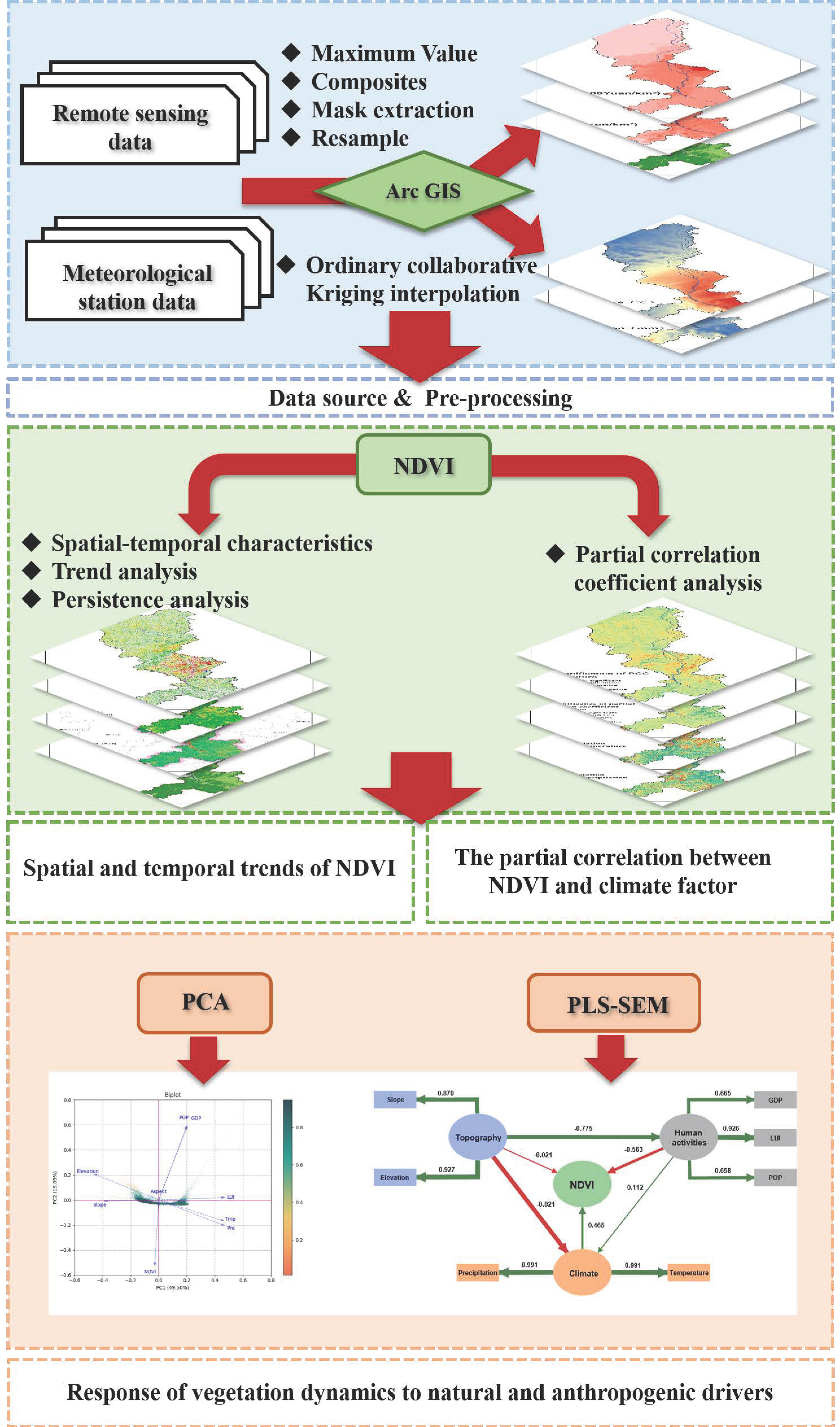
2. Materials and Methods

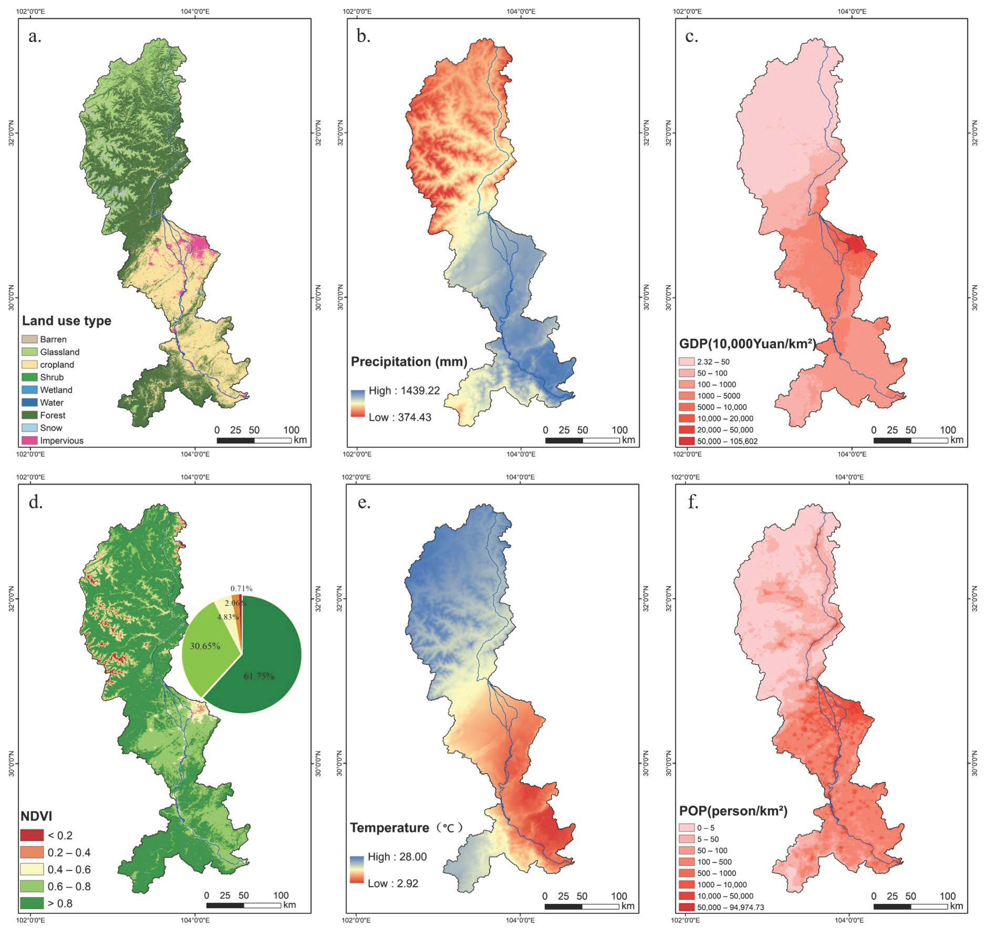
2.1. Study Area

Straddling the confluence of China’s first and second topographical steps, the Minjiang River Basin (MJB) displays a striking elevation range, from a modest 249 m to a towering 6005 m (Figure 1). This dramatic altitude variation not only shapes the landscape but also positions the MJB as a vital ecological buffer for the upper Yangtze River’s tributaries, reinforcing its role in the “Six Rivers” ecological corridors. Covering approximately 44,966 km², the basin constitutes nearly 9.25% of Sichuan Province, with its waters traversing nine of the province’s prefectures. The Minjiang River’s course is divided into three distinct sections: the upper basin which rises above Dujiangyan City, is marked by rugged mountains and deep canyons along the active Longmen Mountains thrust belt—a region known for frequent seismic activities and other geological events. As the river winds southward, it transitions through Dujiangyan down to Leshan, defining the middle reaches before it mellows into the lower reaches, where the landscape softens into expansive plains well-suited for settlement. The elevation range in the upper reaches of the MJB is from 725 to 6005 m, the middle reaches from 321 to 5127 m, and the lower reaches from 249 to 4023 m. Climatically, the MJB features contrasting environments: the upper areas feature a cooler mountain plateau climate, blending temperate and subtropical elements, while the lower regions benefit from a milder subtropical climate with abundant rainfall. This climatic variation is reflected in the basin’s temperature profile, which gently rises from an upstream average annual temperature of 13.9℃ to warmer conditions downstream, accompanied by an average annual precipitation of 995.9 mm, nourishing the rich biodiversity and supporting the complex ecosystems within this critical geographic and ecological junction.

2.2. Data Sources and Processing

This research utilized MOD13Q1 NDVI data from NASA, which are available through the LADS Web MODAPS portal (https://ladsweb.modaps.eosdis.nasa.gov/search/order/1/MOD13Q1--61 (accessed on 13 August 2024)), to examine vegetation dynamics during the growing season (April to October) over the period from 2000 to 2020. The NDVI data, featuring a 16-day temporal resolution and a 250-m spatial resolution, were processed using the Maximum Value Composite method to guarantee high-quality observations. Land use variables necessary for calculating Land Use Intensity (LUI) were obtained from the Chinese Land Cover Dataset (CLCD), created by Huang’s team at Wuhan University (https://zenodo.org/records/12779975 (accessed on 13 August 2024)) and featuring a spatial resolution of 30 m [31]. Topographical variables, including elevation, slope, and aspect, were derived from DEM data from the Geospatial Data Cloud (https://www.gscloud.cn/sources/accessdata/310?pid=1 (accessed on 13 August 2024)), also with a 30-m resolution. Additional environmental data included Population Density (POP) and Gross Domestic Product (GDP) datasets, each with a 1 km resolution, obtained from the Resource and Environment Sciences and Data Center of the Chinese Academy of Sciences (https://www.resdc.cn/Datalist1.aspx?FieldTyepID=8,7 (accessed on 13 August 2024)).

The interpolation method for temperature and precipitation data used ordinary co-kriging from data collected at 26 meteorological stations around the study area (Figure 1). Zhang effectively improved the temperature interpolation results in mountainous areas using this method [32]. Due to the significant elevation differences between the upstream and downstream areas of the MJB, DEM data were selected as a covariate. Ordinary kriging requires the data to follow a normal distribution, with skewness close to 0 and kurtosis close to 3. A log transformation was applied to achieve a normal distribution, resulting in a skewness of 0.03 and a kurtosis of 2.56. Cross-validation was used to evaluate the model’s accuracy: a mean standardized (MS) closer to 0 and a smaller root mean square (RMS) prediction error indicate better model performance; a root mean square standardized (RMST) closer to 1 and an average standard error (ASE) closer to the RMS prediction error indicate an excellent model [33]. In this study, cross-validation showed an MS of −0.003 and an RMST of 1.05, demonstrating the model’s excellence. The interpolation results for temperature and precipitation were resampled to 250 m to match the pixel size of the NDVI data. Figure 2 depicts the spatial distribution of these datasets, which provides essential support for this study.

2.3. Methods

The flowchart of the study is illustrated in Figure 3.

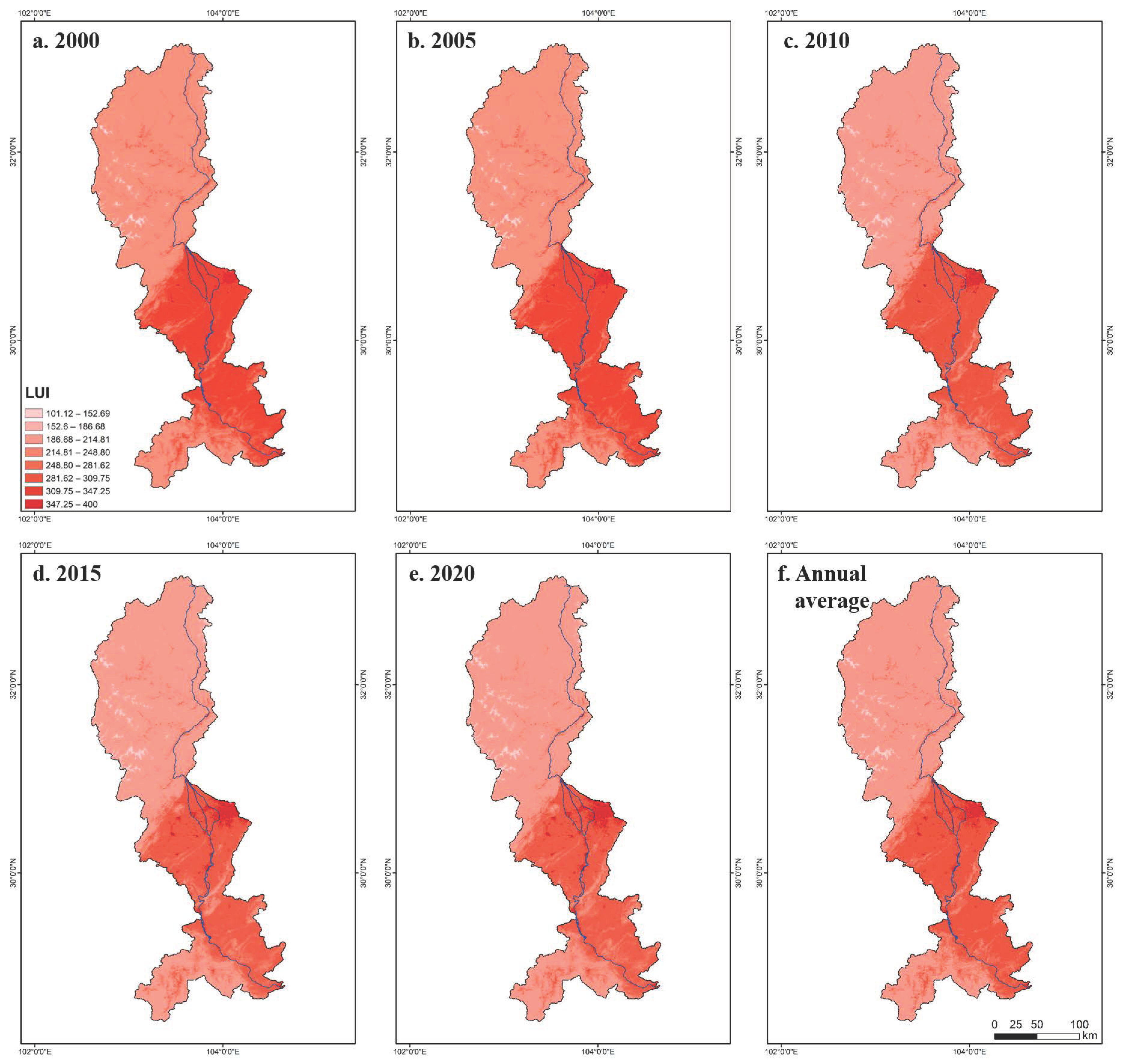
2.3.1. Land Use Intensity

Regarding LUI, it is an indicator that measures the extent of land utilization by human activities. LUI typically reflects the intensity of various activities carried out on the land (such as agricultural, industrial, residential, and commercial uses) and can assist planners and environmental scientists in assessing the sustainability and environmental impact of land use [34]. The formulas are presented below, as follows:

$$\mathit{LUI}=100 \times \left({\sum }_{i=1}^{ n}{P}_i \times { Q}_i\right)$$

(1)

Specifically, the formula Pi represents the intensity level for each land use type (i = 1, 2, 3, 4), which indicates the degree of human impact on the land by assigning weights to each land use type: unused land as level 1, water bodies, forests, and grasslands as level 2, agricultural land as level 3, and construction land as level 4 [35]. Sampling was conducted using a 1 km × 1 km grid. Irregular land parcels larger than 0.5 km² were treated as separate sample units, while those smaller than 0.5 km² were merged with adjacent sample units [36]. Qi denotes the proportion of each land use type in the sample unit area. The variable “n” represents the total number of assessed land use categories. The final LUI pixel size is 1 km × 1 km, consistent with the pixel sizes for GDP and POP.

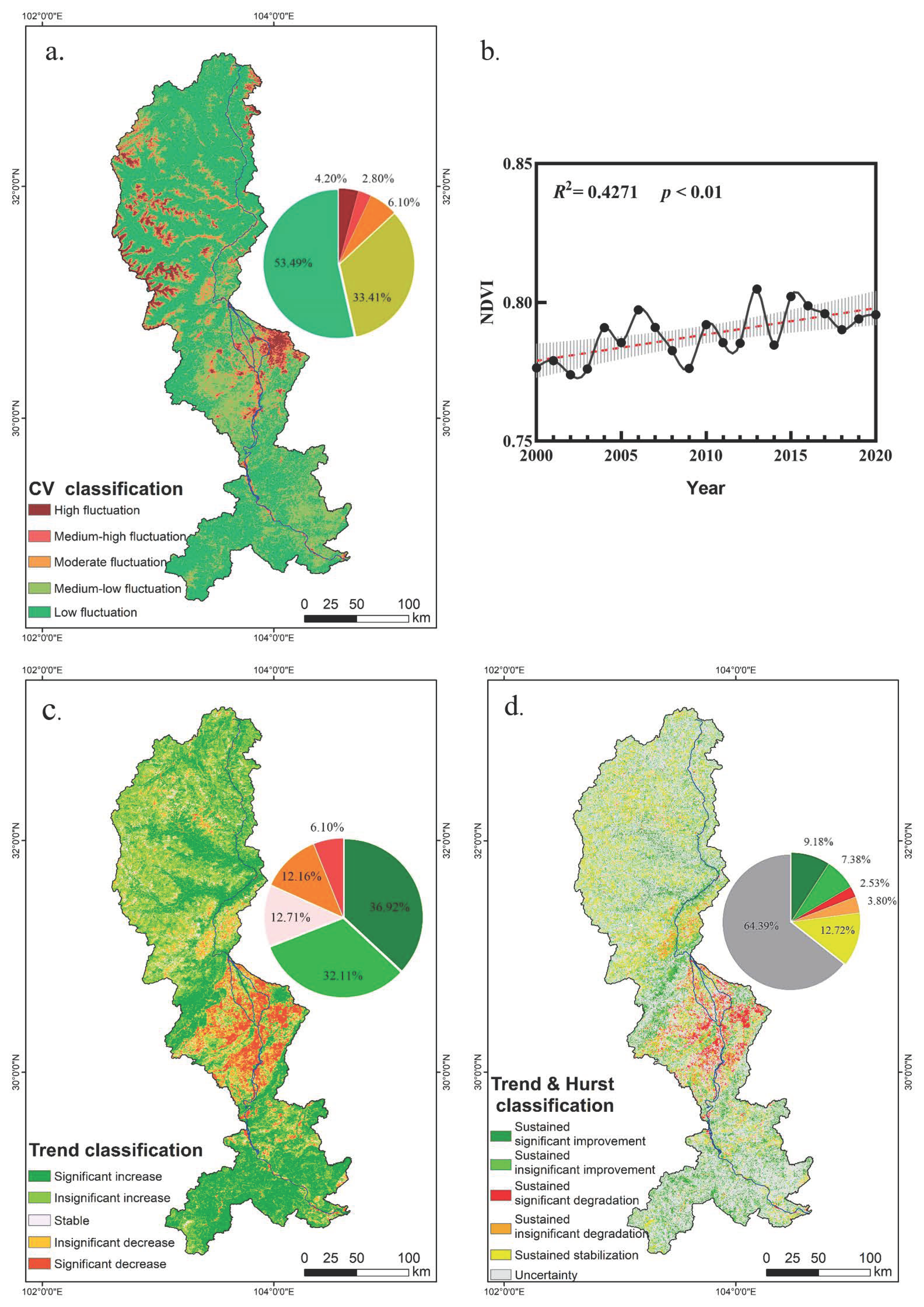
2.3.2. Coefficient of Variation

In statistical analysis, the Coefficient of Variation (CV) is a crucial metric, measuring the degree of variability within a dataset over time. Commonly referred to as the dispersion coefficient, CV is instrumental in gauging the spread of data points around the mean [37]. The study is based on the increase and decrease changes in NDVI calculated on a per-pixel basis, which not only eliminates the need for a reference to the mean value but also neutralizes the measurement scale and dimension lessness. The formulas are presented below, as follows:

$$\mathit{CV}={\displaystyle \frac{{\mathsf{\sigma }}_{\mathit{NDVI}}}{\overline{\mathit{NDVI}}}}$$

(2)

The standard deviation of NDVI is expressed as ${\mathsf{\sigma }}_{\mathit{NDVI}}$. The average value of NDVI is expressed as $\overline{\mathit{NDVI}}$.

2.3.3. Theil–Sen Median Trend Analysis and Mann–Kendall Test

The Theil–Sen Median (T–S) trend analysis and the Mann–Kendall (M–K) test are widely employed for analyzing trends in long-term time series data. Compared to linear regression, they exhibit greater robustness against data errors, effectively mitigate the effects of incomplete time series data and distribution shapes, and demonstrate reduced sensitivity to outliers, thereby enhancing the accuracy of the analysis [38]. The formulas are presented below, as follows:

$$\beta =\mathrm{median}{\displaystyle \frac{\mathit{NDV} I -{\mathit{NDVI}}_j}{k - j}}$$

(3)

In the formula 1 < j < k < n, where i and j represent the time series numbers, NDVI_j and NDVI_k denote the NDVI values at the j-th and k-th time series, respectively. A slope (β) greater than 0 indicates an upward trend, while a slope (β) less than 0 indicates a downward trend. The M–K test, a nonparametric statistical method, is employed to analyze trends in time series data over time. It is not only suitable for non-normally distributed data but also effectively handles outliers. The testing procedure is outlined below, as follows:

$$S={\sum }_{j =1}^{n-1}{\sum }_{k =j+1}^n\mathit{sgn}\left(\theta \right)$$

(4)

$$\mathit{sgn}\left(\theta \right)=\left\{\begin{array}{ll}1& \theta >0\\ 0& \theta =0\\ -1& \theta <0\end{array}\right.$$

(5)

Statistical measures for trend testing are constructed as follows:

$${ Z}_{\mathit{MK}}=\left\{\begin{array}{ll}{\displaystyle \frac{S-1}{\sqrt{\mathit{Var}\left(S\right)}}}& S>0\\ 0& S=0\\ {\displaystyle \frac{S+1}{\sqrt{\mathit{Var}\left(S\right)}}}& S<0\end{array}\right.$$

(6)

In the testing process of Formulas (4)–(6), $\theta ={\mathit{NDVI}}_k-{\mathit{NDVI}}_j$

$$\mathit{Var}\left(S\right)={\displaystyle \frac{n\left(n-1\right)\left(2n+5\right)}{18}}$$

(7)

In the formula, NDVI_j and NDVI_k denote the NDVI values in the j-th and k-th years, respectively; n denotes the length of the time series; and sgn is the sign function. At the significance level α, if |Z_MK| > μ1 − α/2, it indicates a significant change in the research series at the α level. Therefore, this study combines the T–S slope and the M–K test to analyze the trends and significance of NDVI values at the pixel scale within the study area. Based on these analyses, vegetation change trends are categorized into five levels (

Table 1. The proportion of changing trend (%).

β	Z	Classification	Area Ratio
β > 0.0005	1.96 < |Z|	significant increase	36.92
	1.96 ≥ |Z|	insignificant increase	32.11
−0.0005 < β < 0.0005	Z	stable	12.71
β < −0.0005	1.96 ≥ |Z|	insignificant decrease	12.16
	1.96 < |Z|	significant decrease	6.10

).

2.3.4. Hurst Index

The Hurst index is a statistical method used to analyze the self-similarity of time series data and is widely employed across various scientific disciplines, including hydrology, financial market analysis, geology, and climatology. This index assists in determining whether a system or process is persistent, random, or antipersistent [39]. This index has been used to study changes in vegetation cover over the past few decades. The basic principle involves defining the average series for the time series {NDVI(t)}, t = 1, 2, …, n. The formulas are presented below, as follows:

$$\overline{{\mathit{NDVI}}_{\tau } }={\displaystyle \frac{1}{\tau }}{\sum }_{t =1}^{\tau }{\mathit{NDVI}}_{\left(\tau \right)}\hspace{1em}\tau =1, 2, 3\dots , n$$

(8)

Cumulative deviation calculation:

$$X_{\left(t,\tau \right)}=t=1t{\mathit{NDVI}}_{\left(t\right)} -\overline{{ \mathit{NDVI}}_{\tau }}\hspace{1em}1 \ll t \ll \mathrm{\tau }$$

(9)

Range value:

$$R_{\left(\tau \right)}=\underset{1 \ll t \ll \tau }{\mathit{max}}{X}_{\left(t,\tau \right)}-\underset{1 \ll t\ll \tau }{\mathit{min}}{X}_{\left(t,\tau \right)}\hspace{1em}\tau =1, 2, 3\dots , n$$

(10)

Standard deviation calculation:

$${ S}_{\left(\tau \right)}={\left[{\displaystyle \frac{1}{\tau }}{\left({\sum }_{t=1}^{\tau }{\mathit{NDVI}}_{\left(t\right)} -{\mathit{NDVI}}_{\left(\tau \right)}\right)}^2\right]}^{{\displaystyle \frac{1}{2}}}\hspace{1em}\tau =1, 2, 3\dots , n$$

(11)

For ratio “$R_{\left(\mathrm{\tau }\right)}/S_{\left(\mathrm{\tau }\right)}\triangleq R/S$”, if the relationship “$R/S\propto {\tau }^H$” holds, this defines the Hurst phenomenon. The Hurst index (H) is then employed to analyze time series data. The H value is derived by fitting log(R/S) = a + H × log(n) using the least squares method. The value of H indicates the level of randomness or persistence in the NDVI sequence based on the Hurst index classification [40] results of Yuan (

Table 2. The proportion of change trend persistence (%).

Classification	Hurst Index	Trend Persistence Characteristics	Area Ratio
Significant increase Insignificant increase Stable Insignificant decrease Significant decrease	0.5 ≤ H < 1	Sustained significant improvement	9.18
		Sustained insignificant improvement	7.38
		Sustained stable	12.72
		Sustained insignificant degradation	3.80
		Sustained significant degradation	2.53
	0 < H < 0.5	Uncertain	64.39

). The value of H manifests in two forms: if 0.5 ≤ H < l, it suggests that the NDVI time series exhibits sustainability, implying that future changes will align with historical trends, with sustainability intensifying as H approaches 1. If 0 < H ≤ 0.5, it indicates that the long time series NDVI is anti-persistence, where future changes are likely to oppose past trends; the closer H is to 0, the greater the anti-persistence.

2.3.5. Partial Correlation Coefficient Analysis

Numerous studies demonstrate that precipitation and temperature are the key climatic factors influencing regional vegetation growth changes [41,42]. In ecological research, PCC analysis serves as a powerful statistical tool to explore the relationship between two climatic variables while controlling for the potential influence of other variables. This method is crucial for understanding the complex interactions and feedback mechanisms between climate variables, given the inherent complexity and interconnectivity of the climate system. The calculation formula is as follows:

$$r_{\mathit{xy},z}={\displaystyle \frac{r_{\mathit{xy}} -{ r}_{\mathit{xz}}{r}_{\mathit{yz}}}{\sqrt{\left(1-r_{\mathit{xz}}^2\right)\left(1 -r_{\mathit{yz}}^2\right)}}}$$

(12)

In the formula, x, y and z represent NDVI, precipitation, and temperature, respectively; $r_{xy,z}$ denotes the partial correlation coefficient, while $r_{xy}$, $r_{xz}$, and $r_{yz}$ represent the simple correlation coefficients of NDVI with precipitation, NDVI with temperature, and precipitation with temperature, respectively. If $r_{\mathit{xy},z}$ > 0, it means that there is a positive correlation between the two variables, and if $r_{\mathit{xy},z}$ < 0, it indicates a negative correlation.

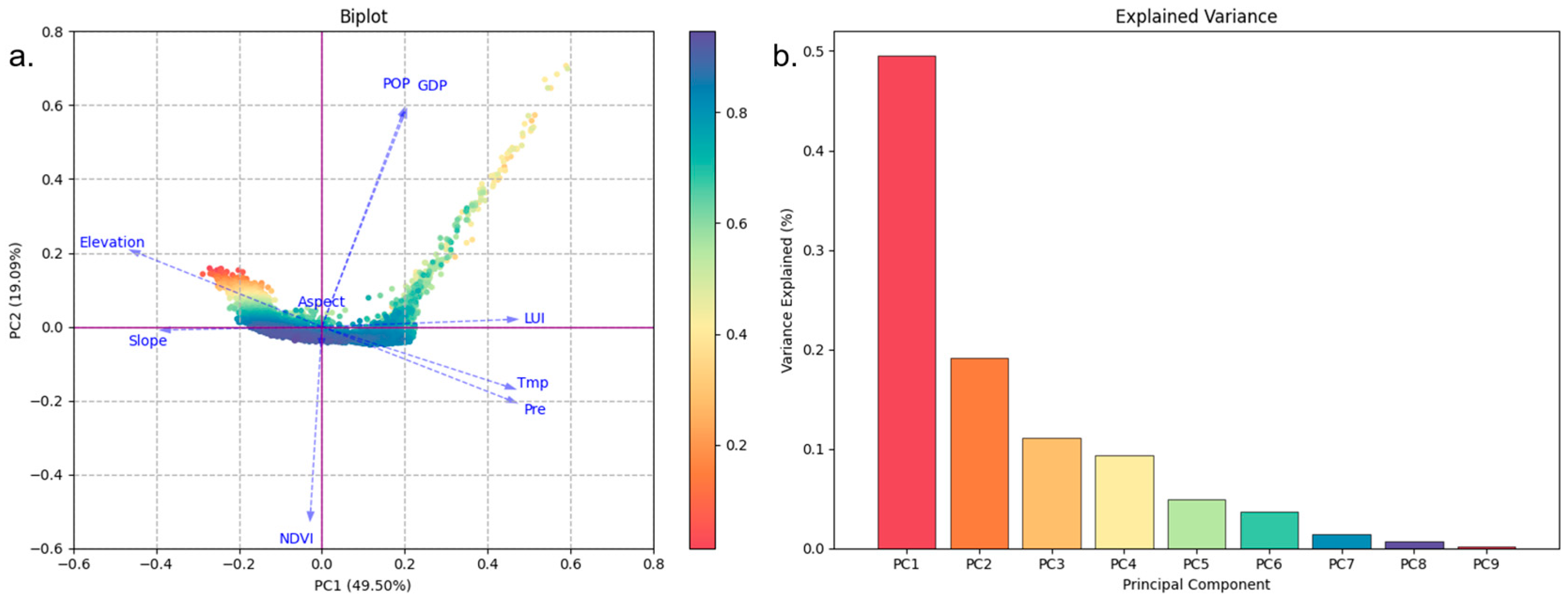
2.3.6. Principal Component Analysis

PCA is a widely used dimensionality reduction technique, primarily employed to map high-dimensional data to lower-dimensional spaces, thereby simplifying the data. The PCA method projects sample data onto the principal component space, which consists of directions with the greatest variance in the data, through a linear transformation. This approach retains the most critical information in the data while reducing its dimensionality. The first principal component accounts for the greatest variance in the data, while each subsequent principal component, constrained to be orthogonal to its predecessors, accounts for the maximum remaining variance [43].

In PCA, loadings represent the projection of the original variables onto the principal components or the linear combination coefficients of each principal component [44]. They reflect the degree of association between the original variables and the principal components. If the angle between two arrows is very small or close to zero, it indicates that these two variables have very similar projection directions in the principal component space. This means that their loadings on these principal components are similar, suggests a high positive correlation in the original data space. Conversely, if the angle between two arrows is close to 180 degrees, it indicates that these two variables have opposite projection directions in the principal component space. This means that their loadings on these principal components are opposite, suggesting a high negative correlation in the original data space. Bartlett’s sphericity test [45] and the Kaiser–Meyer–Olkin (KMO) test [46] were employed to ensure the consistency of PCA. The number of PCs is generally determined based on experience [47] and the cumulative variance percentage of the PCs. A good cumulative variance percentage is typically set around 70% [48,49,50].

In this study, the analysis involves a total of 9 variables, including the dependent variable NDVI and 8 independent factors: Pre, Tmp, Elevation, Aspect, Slope, LUI, POP, and GDP. The formula is as follows:

$$\left[Z_1{Z}_2\cdots Z_m\right]=\left[x_1{x}_2{\cdots x}_n\right]\left[\begin{array}{ccc} y_{11}& y_{21}\cdots & y_{n1}\\ ⋮& \ddots & ⋮\\ { y}_{1n}& y_{2n}\cdots & y_{\mathit{nn}}\end{array}\right]\left(m < n\right)$$

(13)

In this model, x denotes the n-dimensional original data, z signifies the m-dimensional principal components, and y represents the n × m dimensional transformation matrix.

The formula for Bartlett’s test of sphericity is as follows:

$${\chi }^2=-\left(n-1-{\displaystyle \frac{2p+5}{6}}\right)·\ln \left(|\det \left(R\right)|\right)$$

(14)

In the formula, n represents the sample size, p is the number of variables, R is the correlation matrix between variables, and det(R) is the determinant of the correlation matrix. After calculating the ${\chi }^2$ statistic, the corresponding p-value is determined using the cumulative distribution function of the ${\chi }^2$ distribution. If the p-value is less than 0.01, the null hypothesis of sphericity is rejected, indicating that the covariance matrix between the variables is not an identity matrix, meaning that there is correlation among the variables. Otherwise, it is considered that the covariance matrix between the variables is an identity matrix, fitting the sphericity assumption.

The formula for KMO is as follows:

$$\mathit{KMO}={\displaystyle \frac{{\sum }_{i=1}^p{\sum }_{j=1}^p{r}_{\mathit{ij}}^2}{{\sum }_{i=1}^p{\sum }_{j=1}^p{r}_{\mathit{ij}}^2+{\sum }_{i=1}^p{\sum }_{j=1}^p{\left(r_{\mathit{ij}}^2\right)}^2}}$$

(15)

In the formula, r_ij represents the simple correlation coefficient between variables i and j and p denotes the total number of variables. The KMO value typically ranges from 0 to 1, with values closer to 1 indicating higher correlations among variables, making them more suitable for PCA analysis.

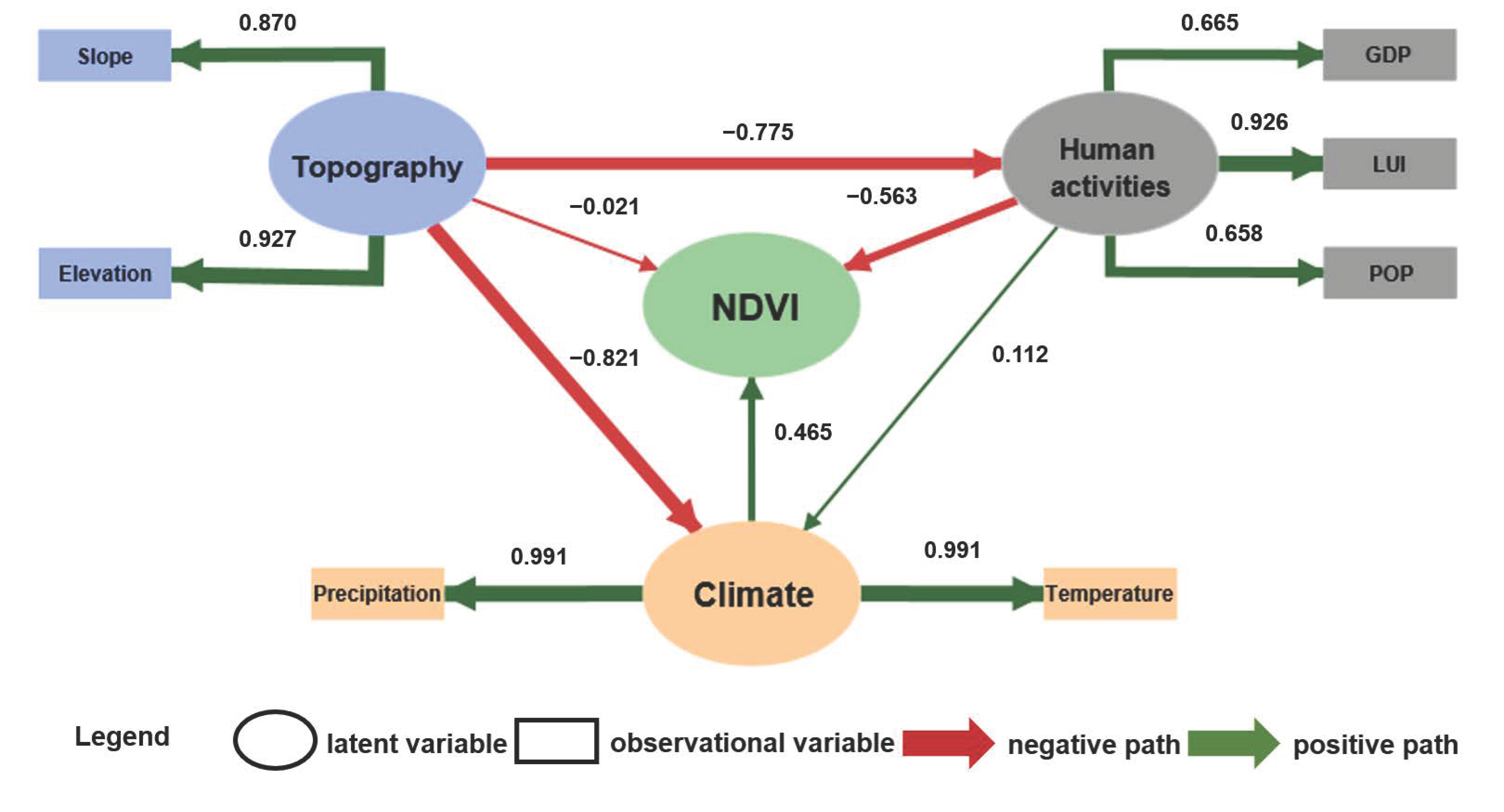
2.3.7. Partial Least Squares Structural Equation Modeling

Recently, the PLS-SEM method has gained popularity for modeling complex relationships among multiple variables simultaneously. PLS-SEM provides more flexibility compared to traditional covariance-based structural equation modeling methods like AMOS or LISREL, making it especially suitable for analyzing non-normal data and performing predictive studies. It is widely applied across diverse fields including business, marketing, management, social sciences, environmental research, and healthcare [51,52]. PLS-SEM estimates path coefficients by constructing systems of observed and latent variables within theoretical models.

In this study, the structural equation model was constructed using Smart PLS 4.0 software. First, 10,000 points were randomly sampled using ArcGIS 10.7 version, with constraints on the sampling extent and a minimum allowed distance of 1 km to ensure that the random points were within the study area and not overly dense. Then, bootstrapping was used to evaluate the significance of the path coefficients [53].

In the construction of causal paths in structural equation modeling, the prerequisite is that there should be a theoretical basis for the interactions between influencing factors [54]. Given the frequent occurrence of air pollution issues resulting from industrial development and urban expansion [55,56] and the complex terrain of the MJB that limits human activities and promotes the formation of regional microclimates in mountainous and canyon areas [11,57], we propose the following three hypotheses: (1) terrain factors indirectly influence NDVI by affecting climatic patterns; (2) natural elements shape human activities; and (3) human activities alter the climate. The coefficient of determination (R²) and the Stone-Geisser coefficient (Q²) [58] were chosen to evaluate the performance of the model. The model fit (GOF) further indicates the overall fit of the PLS-SEM model. This metric integrates the model’s explanatory (R²) and predictive (Q²) capabilities, offering a comprehensive evaluation of the model’s effectiveness [58,59] (

Table 3. PLS-SEM evaluation index standard.

Index Standard	Value	Classification
R2	>0.67	High explanatory power
	>0.33	Moderate explanatory power
	>0.19	Low explanatory power
Q2	>0	The larger the value, the higher the prediction accuracy of the model.
GOF	0.1	Low model fitting
	0.25	Medium model fitting
	0.36	High model fitting

).

3. Results

3.1. Spatiotemporal Variation Analysis of LUI

Figure 4 shows the spatial distribution pattern of LUI. The overall distribution pattern of LUI indicates high values in the Chengdu Plain in the middle reaches and low values in the high-altitude areas upstream and the plains downstream. From 2000 to 2020, the LUI values in the Chengdu Plain area increased and became more concentrated, while the changes in LUI in the upstream and downstream regions were not significant.

3.2. Spatiotemporal Variation and Trend Analysis of NDVI

3.2.1. Time Variation Characteristics

From 2000 to 2020, the average annual NDVI in the MJB showed a fluctuating upward trend (Figure 5b). The average annual growth rate of NDVI during the growing season in the MJB was 0.95 × 10⁻³ per year (p < 0.01). Notably, NDVI increased significantly between 2000–2005 and 2010–2015 but it declined continuously from 2008 to 2010. Over the two decades, the annual mean NDVI in the MJB ranged from 0.773 to 0.805, with the lowest value recorded in 2002 and the highest in 2013. Overall, these findings indicate a sustained improvement in the region’s vegetation cover and health over the past twenty years.

3.2.2. Spatial Distribution Characteristics

The spatial distribution pattern and graded area percentage of average NDVI from 2000 to 2020 are shown in Figure 2a. For statistical segmentation in this study, areas with NDVI values below 0.2 accounted for 0.71%, primarily located in the glacial deserts and mountain plateaus of the upper Minjiang River, characterized typically by sparse vegetation, predominantly grasslands, and alpine meadows. Regions with NDVI values ranging from 0.2 to 0.4, accounting for 2.06%, were primarily concentrated in the Chengdu Plain of the middle MJB and high-altitude regions of the upper river. Areas with NDVI values between 0.4 and 0.6 accounted for 4.83%, while areas with values between 0.6 and 0.8 comprised 30.65%, mainly located in the middle and lower MJB. The largest proportion of areas, with NDVI values greater than 0.8 at 61.75%, were predominantly in lower altitude regions of the upper MJB and other high NDVI value areas in the lower MJB, indicating ample vegetation cover and better ecological conditions.

This paper calculated the NDVI of MJB from 2000 to 2020. The spatial distribution of the coefficient of variation (Figure 5a) ranges from 0 to 2.11, with an average value of 0.066, indicating that the overall NDVI variability of the entire MJB is relatively low, although there are significant fluctuations in specific local areas. Regarding spatial distribution patterns, variability is greater in the high-altitude mountainous areas of the northwestern upstream and the Chengdu Plain in the eastern downstream, while it is smaller in the low-altitude mountainous areas of the northeastern upstream and the southern Sichuan region downstream. The area with low variability accounted for 53.49%, while medium–low, medium, and high variability areas constituted 33.41%, 6.10%, and 7.00%, respectively.

3.2.3. Trend Analysis of Long-Time Series NDVI

Figure 5c shows that the NDVI in the MJB from 2000 to 2020 exhibited significant spatial heterogeneity, with the NDVI trend classification and area percentages detailed in Table 1. Around 69.03% of the total area displayed an improving NDVI trend, 18.26% exhibited a degrading trend, and the remaining 12.71% remained stable. Notably, about 36.92% of the region where NDVI showed marked improvement was primarily distributed in the western Sichuan area of the upper MJB and the southern Sichuan area of the lower MJB. In contrast, areas where vegetation NDVI is severely degraded account for 6.10% of the total study region and are primarily concentrated in the Chengdu Plain. This degradation centered on Chengdu City and spread to surrounding areas including Meishan and Ya’an.

3.2.4. Predictability of Long Time Series of NDVI

The coupled results of trend analysis and Hurst index (Figure 5d and Table 2) are divided into six scenarios: persistence with a significant decrease; persistence with a slight decrease; persistence with stability; persistence with a slight increase; persistence with a significant increase; and uncertain future trends, which include combinations of counter-persistence with severe degradation, slight degradation, stability, slight improvement, and notable improvement, complicating predictions of future trends. Overlaying the Theil–Sen Median results with the Hurst index indicated that the area with uncertain trends was the largest (64.39%), with persistently stable areas accounting for 12.72%, persistently degrading areas comprising 6.33% (slight degradation 3.80%, severe degradation 2.53%, primarily in the Chengdu Plain), and persistently improving areas constituting 16.56% (slight improvement 7.38%, significant improvement 9.18%), predominantly in the lower-altitude regions of the upper MJB and downstream areas.

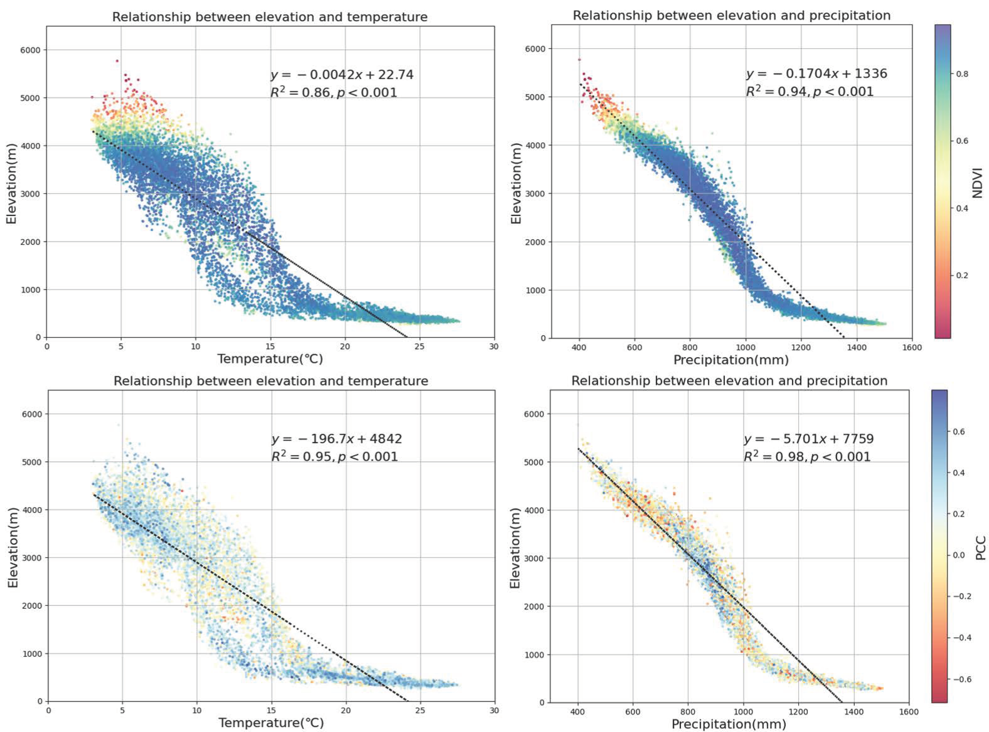
3.3. Relationship between Climate Factors and NDVI

A partial correlation analysis of NDVI and annual precipitation data was conducted using MATLAB R2016a version, with the partial correlation coefficient ranging from −0.81 to 0.88 (Figure 6a). As shown in Figure 6b and

Table 4. The partial correlation analysis results (%).

Classification	Area Ratio (Precipitation)	Area Ratio (Temperature)
Extremely significant negative correlation	0.74	0.56
Significant negative correlation	1.67	1.82
No significant negative correlation	31.64	34.79
No significant positive correlation	54.46	56.54
Significant positive correlation	6.80	4.83
Extremely significant positive correlation	4.69	1.44

, areas where vegetation NDVI is positively correlated with precipitation account for 65.95% of the MJB. Of these, areas with extremely significant positive correlations make up 4.69%, significantly positive correlations cover 6.80%, and non-significant positive correlations comprise 54.46%. In contrast, areas negatively correlated with precipitation account for 34.05% of the MJB. Among these, extremely significant negative correlations constitute 0.74%, significant negative correlations account for 1.67%, and non-significant negative correlations cover 31.64%. Spatial analysis indicates that areas where vegetation NDVI is significantly positively correlated with precipitation are primarily found in the low-altitude valleys upstream and the southeastern plains downstream; the region showing a negative correlation is predominantly located in the Chengdu Plain, situated in the lower part of the MJB.

A partial correlation analysis of NDVI and annual temperature data was conducted using MATLAB R2016a version, with the partial correlation coefficient ranging from −0.93 to 0.90 (Figure 6d). As shown in Figure 6e and Table 4, areas where vegetation NDVI is positively correlated with temperature account for 62.83% of the MJB. Of these, areas with extremely significant positive correlations make up 1.44%, significantly positive correlations cover 4.83%, and non-significant positive correlations comprise 56.54%. In contrast, areas negatively correlated with temperature account for 37.17% of the MJB. Among these, extremely significant negative correlations constitute 0.56%, significant negative correlations account for 1.82%, and non-significant negative correlations cover 34.79%. Spatially, areas positively correlated between vegetation NDVI and temperature were primarily located in the southwestern region of the lower MJB and scattered across the upper MJB, whereas negatively correlated areas predominantly lay in the Chengdu Plain of the lower MJB and were dispersed throughout the upper MJB.

By conducting zonal statistics on the PCC with vegetation growth trends, the following results were obtained (

Table 5. Partial correlation coefficients corresponding to vegetation growth trends.

Classification	Average Precipitation PCC	Average Temperature PCC
significant increase	0.235	0.138
insignificant increase	0.103	0.076
stable	0.014	0.026
insignificant decrease	−0.071	−0.013
significant decrease	−0.169	−0.085

). Pixels exhibiting significant vegetation growth had the highest average PCC, with an average precipitation PCC of 0.235 and an average temperature PCC of 0.138. Pixels showing significant vegetation degradation had the lowest average PCC, with an average precipitation PCC of −0.169 and an average temperature PCC of −0.085. Pixels with stable vegetation growth exhibited an average PCC close to zero, with an average precipitation PCC of 0.014 and an average temperature PCC of 0.026. Pixels with insignificant vegetation growth had an average precipitation PCC of 0.103 and an average temperature PCC of 0.076. Pixels with insignificant vegetation degradation had an average precipitation PCC of −0.071 and an average temperature PCC of −0.013.

To further investigate the relationship between NDVI and climatic variables, we randomly selected 10,000 sampling points (consistent with Section 2.3.7). For each point, the correlation coefficient between NDVI and climatic variables was calculated. A quadratic polynomial curve is used to fit the relationship between NDVI and climate factors. NDVI is significantly correlated with precipitation (p < 0.001). The relationship between NDVI and precipitation weakens when precipitation is below or exceeds 1000 mm (Figure 6c), with NDVI being highest at around 1000 mm of precipitation. This indicates that vegetation growth is most sensitive to annual precipitation of approximately 1000 mm. As precipitation increases, the relationship between NDVI and precipitation becomes more apparent; beyond this threshold, further increases in precipitation do not lead to higher NDVI. This suggests that the water resource utilization capacity of vegetation may be limited or increased precipitation may reduce temperature and sunlight levels. Similarly, NDVI is significantly correlated with temperature (p < 0.001). The relationship between NDVI and temperature weakens when the temperature is below or exceeds approximately 20 °C (Figure 6e), as both low and high temperatures inhibit vegetation growth.

3.4. PCA and PLS-SEM Analysis

The results of Bartlett’s test of sphericity and the KMO test showed a p-value of less than 0.01 and a KMO value of more than 0.80, indicating that the data are suitable for PCA analysis. The PCA method is used to decompose the nine parameters into PC1 (49.50%) and PC2 (19.09%) (Figure 7b). Figure 7a shows that PC1 has the greatest influence on precipitation (Pre), temperature (Tmp), and elevation, while aspect has the least influence. The absolute value ranking of PC1 is Elevation > Pre > Tmp > LUI > Slope > GDP > POP > Aspect. On PC2, the ranking is GDP > POP > Elevation > Pre > Tmp > LUI > Slope > Aspect (with NDVI as the reference variable, it is not included in the component ranking). The angles between the variables indicate the correlations between different dimensions. If the angle between two variables is less than 90 degrees, it indicates a positive correlation; if the angle is greater than 90 degrees, it indicates a negative correlation. The size of the angle between NDVI and other variables is Pre < Tmp < Slope < LUI < Elevation < GDP < POP < Aspect. Since the weight of PC1 (49.50%) is significantly greater than that of PC2 (19.09%) (Figure 7b), the weight of PC2 only supplements PC1 in explaining the variation in weight. Therefore, when considering the weight and angle ranking, the main factors affecting changes in the vegetation index are elevation, temperature, precipitation, and LUI.

The results of the principal component analysis provide a qualitative interpretation of the relationship between the NDVI and influencing factors, though this relationship is somewhat unclear. Therefore, PLS-SEM is employed for a quantitative analysis of vegetation NDVI’s response to natural and anthropogenic drivers (Figure 8). The path between aspect and terrain did not pass the significance test and was therefore excluded. As shown in

Table 6. The model performance of the PLS-SEM.

Indicators	Type	Value
R2	NDVI	0.141
	Human activities	0.601
	Climate factors	0.828
Q2	/	0.140
GOF	/	0.458
p-value	Topographic factors → NDVI	0.391
	Human activities → NDVI	0.000
	Climate factors → NDVI	0.000

, PLS-SEM has good performance, with its Q² being greater than 0, indicating that the model can effectively predict endogenous latent factors. The GOF value indicates a high overall quality. Moreover, except for topographic factors, p-values were below 0.001, signifying significant path coefficients; this may be due to the significant elevation differences in the upper and lower reaches of the MJB. Path coefficients facilitate the examination of interactions among latent variables. Climate factors directly influence vegetation growth, with a total effect of 0.465. The direct impact of terrain on vegetation growth is minimal, with a total effect of −0.021, indicating a negative correlation, primarily influenced by elevation, whose path coefficient to climatic factors is −0.821, primarily affecting vegetation growth indirectly through the climate. The total impact of human activities on vegetation growth is −0.563. Among the three latent variables representing human activities, LUI has the largest path coefficient (0.926), indicating that LUI is the primary factor representing the impact of human activities on NDVI trend changes. Compared to GDP and POP, LUI has a more significant influence.

4. Discussion

4.1. Spatiotemporal Variation in NDVI

This study examines the long-term series of vegetation NDVI from 2000 to 2020, revealing an overall upward trend (Figure 5b). However, the significant decline in NDVI from 2008 to 2010 is closely related to the “5.12” Great Earthquake in 2008. The earthquake triggered numerous landslides and debris flows, damaging approximately 1200 km² of vegetation [60], with vegetation coverage in the hardest-hit cities and counties decreasing by about 4.7% [61]. After 2010, vegetation NDVI increased, benefiting from government-implemented ecological restoration measures post-earthquake that facilitated the recovery of basin vegetation [62]. According to T–S trend analysis and the M–K test, vegetation improvements in the MJB were primarily observed in the upper and lower regions of the MJB, while significant degradation occurred in the Chengdu Plain, a finding supported by studies from Wu and others [63,64]. Vegetation changes in the MJB show significant regional disparities, with improvements in the upper and lower regions contrasting sharply with degradation in the Chengdu Plain, likely due to lower population density and reduced land development intensity in these areas. Conversely, high urbanization and intensive agricultural activities in the Chengdu Plain may have exacerbated vegetation degradation, aligning with observations by Enans and Geerken’s study on the direct effects of human activities on vegetation dynamics [65]. Furthermore, research by Kerr and Ostrovsky has identified agricultural expansion and urbanization as primary drivers of global forest cover and biodiversity loss [66]. Human-driven land use change affects vegetation dynamics in the basin, such as in other basins such as Poyang Lake [67] and the lower Yangtze River Basin [68].

4.2. The Influence of Climate and Terrain on Vegetation Growth

An important phenomenon is the influence of elevation gradients and climatic factors on the distribution patterns of vegetation. Elevation indirectly moderates how climatic conditions like temperature and precipitation impact vegetation growth [69]. In high mountain and canyon zones, terrain features shape regional microclimates, significantly impacting vegetation growth indirectly [57]. Figure 8 illustrates the relationship between NDVI, PCC, climatic factors, and elevation. Firstly, an elevation of 4000 m is critical for vegetation growth in the MJB; irrespective of climate, areas above 4000 m in elevation show a notable decrease in NDVI. Increased altitude enhances evaporation due to warming and strong radiation, directly impacting vegetation’s water use efficiency. Research by Piao suggests that changes in precipitation and temperature significantly affect grassland vegetation growth [41]. Jobbagy observed that in arid regions, water availability predominantly constrains vegetation productivity [70]. As depicted in Figure 5f, vegetation exhibits a nonlinear response to temperature, influenced significantly only when temperatures deviate from a critical range [71]. Here, the critical temperature range of 15–20 °C is pivotal, with vegetation greenness decreasing as temperatures move beyond this range. Additionally, in regions where precipitation is below 600 mm, overall vegetation greenness is reduced and the water demand for typical vegetation growth is compromised (Figure 9).

From the perspective of PCC, there are specific temperature thresholds under various elevation gradients (Figure 9). When temperature surpasses this threshold, it either inhibits or promotes vegetation growth. Particularly, in lowland areas below 1000 m in elevation, temperatures exceeding 15 °C typically foster vegetation growth; conversely, in regions above 3000 m in elevation, temperatures surpassing 5 °C begin to impede vegetation growth. Some past studies have shown that sub-zero temperatures may directly cause damage to plant cells [72]. In regions spanning from 1500 to 4000 m in elevation, vegetation growth is most sensitive when precipitation is between 800 and 1000 mm, and during this range, precipitation has the most significant promoting effect on vegetation growth. When rainfall exceeds 1000 mm, vegetation development is inhibited. Previous studies have shown that excessive precipitation can inhibit vegetation growth, as surpassing a certain rainfall threshold can increase cloud cover and reduce sunlight availability for vegetation [73], which aligns with our analysis. When rainfall is below 800 mm, its inhibitory effect on vegetation development progressively intensifies with higher elevations. Under specific climatic thresholds, limited water availability becomes the primary constraint on vegetation growth, with high temperatures enhancing respiration, accelerating nutrient consumption, increasing transpiration, and reducing organic matter accumulation, thereby slowing growth [70,74].

4.3. The Interrelation of the Impact Factor

Currently, there is widespread recognition that vegetation growth is a multifaceted process influenced by numerous driving factors. In the MJB, with its significant topographical variations and delicate ecological environment, the influence of terrain and human activities cannot be overlooked. As depicted in Figure 7, the primary factors influencing NDVI include elevation, temperature, precipitation, and land use intensity. The PLS-SEM findings further corroborate these connections and measure the proportional impacts of each factor (Figure 8). Of these variables, human activities have the most significant direct impact on NDVI, with a coefficient of −0.563. Seto observed that urban expansion directly compromises ecosystem services [75]. Research conducted by Yang [31] and Xu [76], employing PLS-SEM, has verified that topographic factors play a significant role in vegetation growth, which is in line with the findings of this study.

4.4. Limitation

While this study provides important insights into the dynamic changes in vegetation in the MJB, it is restricted by limitations in data resolution and coverage. This research exclusively employs MODIS products, which have a spatial resolution of 250 m, to calculate NDVI over the past 20 years. Given the relatively short observation period and low spatiotemporal resolution, this dataset may not fully capture the finer details of vegetation changes, thereby not meeting the requirements for long-term ecological monitoring.

Due to the small size of our study area, there is no available public meteorological data with a resolution consistent with NDVI. Therefore, we used data from meteorological stations. Furthermore, the acquisition of climate data is potentially compromised by uneven station distribution, particularly in mountainous regions with complex terrain, where station representativeness is likely inadequate.

Moreover, although different statistical methods were employed to analyze the data, the underlying assumptions of these models and the uncertainties within the input data might impact the accuracy of the results. Due to different climatic conditions and human activities, vegetation may undergo nonlinear changes, as previous studies have indicated [77,78]. This study does not fully consider the nonlinear trends to examine the impact of parameters, especially human activities. Such an analysis could provide a deeper understanding of the impact of human activities on vegetation cover in the future.

As machine learning and artificial intelligence technologies continue to advance, their application in environmental and ecological sciences promises to enhance both the efficiency and precision of complex data analyses. By adopting enhanced monitoring techniques and advanced analytical methods, future research could provide a more robust scientific foundation for developing effective environmental management policies and sustainable development strategies.

5. Conclusions

This research employs T–S trend analysis, PCC, PLS-SEM, and PCA to examine the factors affecting vegetation dynamics in the MJB. The main findings are summarized as follows:

(1) The overall vegetation in the MJB exhibited significant growth, with an average NDVI growth rate of 0.95 × 10⁻³ per year (p < 0.01). Areas with low NDVI values are predominantly found in the high-altitude mountain regions upstream and in the Chengdu Plain midstream, whereas high NDVI values characterize the low-altitude regions upstream and downstream of urban areas such as Leshan, Zigong, and Yibin. The distribution pattern of NDVI fluctuations is characterized by high variability in the upstream northwest high-altitude mountain areas and the midstream Chengdu Plain, while lower variability marks the upstream northeast mid-low altitude mountain areas and the downstream southern Sichuan region. The NDVI trends in the MJB indicate both improvement and degradation. Approximately 69.03% of the area, primarily in the western and southern Sichuan regions, exhibits improvement, whereas degradation predominantly occurs in the Chengdu Plain. Trend analysis and Hurst coupling results reveal that the largest proportion of the area is uncertain (64.39%), with stable areas constituting 12.72%, and zones of persistent improvement, accounting for 16.56%, predominantly located in the low-altitude upstream regions and the southern downstream area.

(2) NDVI exhibits a strong positive correlation with climate in the MJB. Specifically, areas positively correlated with precipitation and temperature accounted for 65.95% and 62.83%, respectively, while negatively correlated areas accounted for 34.05% and 37.17%. The areas with significant vegetation growth had the highest average PCC, while the areas with significant vegetation degradation had the lowest average PCC. Vegetation growth is heavily impacted by critical thresholds for temperature and precipitation. Specifically, vegetation growth is inhibited when temperatures fall below or exceed 15–20 °C and similarly, when precipitation levels are below or exceed 1000 mm.

(3) The overall effects of climatic factors, topographic influences, and human activities on vegetation growth in the MJB are measured at 0.465, −0.021, and −0.563, respectively. Topography and human activities have indirect effects on vegetation growth by influencing climatic conditions, with their impacts quantified at −0.821 and 0.112, respectively. The more pronounced effect of topography indicates its critical role in shaping climatic conditions. Additionally, topography significantly influences the scope of human activities, with a quantified impact of −0.775. Among these three factors, human activities, particularly through LUI, emerge as the most significant drivers of change, profoundly affecting vegetation dynamics in the basin.

References

1. Keenan, T.F.; Riley, W.J. Greening of the land surface in the world’s cold regions consistent with recent warming. Nat. Clim. Chang. 2018, 8, 825–828. [Google Scholar] [CrossRef] [PubMed]
2. Piao, S.; Wang, X.; Park, T.; Chen, C.; Lian, X.; He, Y.; Bjerke, J.W.; Chen, A.; Ciais, P.; Tommervik, H.; et al. Characteristics, drivers and feedbacks of global greening. Nat. Rev. Earth Environ. 2020, 1, 14–27. [Google Scholar] [CrossRef]
3. Liu, Y.; Zhang, X.; Du, X.; Du, Z.; Sun, M. Alpine grassland greening on the Northern Tibetan Plateau driven by climate change and human activities considering extreme temperature and soil moisture. Sci. Total Environ. 2024, 916, 169995. [Google Scholar] [CrossRef]
4. Piao, S.; Fang, J.; Zhou, L.; Guo, Q.; Henderson, M.; Ji, W.; Li, W.; Tao, S. Interannual variations of monthly and seasonal NDVI in China from 1982 to 1999. J. Geophys. Res. Atmos. 2003, 108, 4401. [Google Scholar] [CrossRef]
5. Nemani, R.R.; Keeling, C.D.; Hashimoto, H.; Jolly, W.M.; Piper, S.C.; Tucker, C.L.; Myneni, R.B.; Running, S.W. Climate-driven increases in global terrestrial net primary production from 1982 to 1999. Science 2003, 300, 1560–1563. [Google Scholar] [CrossRef]
6. Lehnert, L.; Wesche, K.; Trachte, K.; Bendix, J. Climate variability rather than overstocking causes recent large scale cover changes of Tibetan pastures. Sci. Rep. 2016, 6, 24367. [Google Scholar] [CrossRef]
7. Ran, Q.; Hao, Y.; Xia, A.; Liu, W.; Hu, R.; Cui, X.; Xue, K.; Song, X.; Xu, C.; Ding, B.; et al. Quantitative assessment of the impact of physical and anthropogenic factors on vegetation spatial-temporal variation in northern Tibet. Remote Sens. 2019, 11, 1183. [Google Scholar] [CrossRef]
8. Jiang, Z.; Hu, Z.; Lai, D.; Han, D.; Wang, M.; Liu, M.; Zhang, M.; Guo, Y. Light grazing facilitates carbon accumulation in subsoil in Chinese grasslands:a meta-analysis. Glob. Chang. Biol. 2020, 26, 7186–7197. [Google Scholar] [CrossRef]
9. Haberl, H.; Erb, K.H.; Krausmann, F.; Gaube, V.; Bondeau, A.; Plutzar, C.; Gingrich, S.; Lucht, W.; Fischer-Kowalski, M. Quantifying and mapping the human appropriation of net primary production in earth’s terrestrial ecosystems. Proc. Natl. Acad. Sci. USA 2007, 104, 12942–12947. [Google Scholar] [CrossRef] [PubMed]
10. Song, X.; Hansen, M.C.; Stehman, S.V.; Potapov, P.V.; Tyukavina, A.; Vermote, E.F.; Townshend, J.R. Global land change from 1982 to 2016. Nature 2018, 560, 639–643. [Google Scholar] [CrossRef]
11. Huang, Y.; Xin, Z.; Dor-ji, T.; Wang, Y. Tibetan Plateau greening driven by warming-wetting climate change and ecological restoration in the 21st century. Land Degrad. Dev. 2022, 33, 2407–2422. [Google Scholar] [CrossRef]
12. Wang, B.; Xu, G.; Li, P.; Zhang, Y.; Cheng, Y.; Jia, L.; Zhang, J. Vegetation dynamics and their relationships with climatic factors in the Qinling Mountains of China. Ecol. Indic. 2020, 108, 105719. [Google Scholar] [CrossRef]
13. Zhang, J.; Sun, J.; Ma, B.; Du, W. Assessing the ecological vulnerability of the upper reaches of the Minjiang River. PLoS ONE 2017, 12, e0181825. [Google Scholar] [CrossRef]
14. Han, J.; Huang, Y.; Zhang, H.; Wu, X. Characterization of elevation and land cover dependent trends of NDVI variations in the Hexi region, northwest China. J. Environ. Manag. 2019, 232, 1037–1048. [Google Scholar] [CrossRef]
15. Huang, K.; Zhang, Y.; Zhu, J.; Zhao, W. The influences of climate change and human activities on vegetation dynamics in the Qinghai-Tibet plateau. Remote Sens. 2016, 8, 876. [Google Scholar] [CrossRef]
16. Dong, S.; Shang, Z.; Gao, J.; Boone, R.B. Enhancing the ecological services of the Qinghai-Tibetan Plateau’s grasslands through sustainable restoration and management in era of global change. Agric. Ecosyst. Environ. 2022, 326, 107756. [Google Scholar] [CrossRef]
17. Seddon, N.; Chausson, A.; Berry, P.; Girardin, C.A.J.; Smith, A.; Turner, B. Understanding the value and limits of nature-based solutions to climate change and other global challenges. Philos. Trans. R. Soc. B Biol. Sci. 2020, 375, 20190120. [Google Scholar] [CrossRef]
18. Yao, T.; Bolch, T.; Chen, D.; Gao, J.; Immerzeel, W.; Piao, S.; Su, F.; Thompson, L.; Wada, Y.; Wang, L.; et al. The imbalance of the Asian water tower. Nat. Rev. Earth Environ. 2022, 3, 618–632. [Google Scholar] [CrossRef]
19. Sun, P.; Liu, S.; Jiang, H.; Lue, Y.; Liu, J.; Lin, Y.; Liu, X. Hydrologic effects of NDVI time series in a context of climatic variability in an Upstream Catchment of the Minjiang River. J. Am. Water Resour. 2008, 44, 1132–1143. [Google Scholar] [CrossRef]
20. Zhang, M.; Wei, X.; Sun, P.; Liu, S. The effect of forest harvesting and climatic variability on runoff in a large watershed: The case study in the upper Minjiang River of Yangtze River basin. J. Hydrol. 2012, 464, 1–11. [Google Scholar] [CrossRef]
21. Li, C.; Liu, L.; Sun, P.A. Study on the Relationship Between Vegetation Pattern and Environment in the Upstream of Minjiang River. J. Beijing Norm. Univ. 2005, 4, 404–409. (In Chinese) [Google Scholar] [CrossRef]
22. Fu, B.; Xu, P.; Wang, Y.; Peng, Y.; Ren, J. Spatial Pattern of Water Retetnion in Dujiangyan County. Acta Ecol. Sin. 2013, 33, 789–797. (In Chinese) [Google Scholar]
23. Zhu, C.; Zhang, J.; Zhao, Y.; Liu, C. Topographic gradient effects of ecosystem services in a typical watershed in the eastern margin of the Qinghai-Tibet Plateau: A case study of the upper reaches of the Minjiang River. Resour. Environ. Yangtze Basin 2017, 26, 1687–1699. (In Chinese) [Google Scholar]
24. Xiong, Y.; Wang, H. Spatial relationships between NDVI and topographic factors at multiple scales in a watershed of the Minjiang River, China. Ecol. Inform. 2022, 69, 101617. [Google Scholar] [CrossRef]
25. Wang, J.; Fan, Y.; Yang, Y.; Zhang, L.; Zhang, Y.; Li, S.; Wei, Y. Spatial-temporal evolution characteristics and driving force analysis of ndvi in the minjiang river basin, china, from 2001 to 2020. Water 2022, 14, 2923. [Google Scholar] [CrossRef]
26. Wang, G.; Peng, W. Quantifying spatiotemporal dynamics of vegetation and its differentiation mechanism based on geographical detector. Environ. Sci. Pollut. Res. 2022, 29, 32016–32031. [Google Scholar] [CrossRef]
27. Tucker, C.J. Red and photographic infrared linear combinations for monitoring vegetation. Remote Sens. Environ. 1979, 8, 127–150. [Google Scholar] [CrossRef]
28. Chen, Y.; Zhang, T.; Zhu, X.; Yi, G.; Li, J.; Bie, X.; Hu, J.; Liu, X. Quantitatively analyzing the driving factors of vegetation change in China: Climate change and human activities. Eco. Inform. 2024, 82, 102667. [Google Scholar] [CrossRef]
29. Wu, C.; Wang, X.; Wang, H.; Ciais, P.; Penuelas, J.; Myneni, R.B.; Desai, A.R.; Gough, C.M.; Gonsamo, A.; Black, A.T.; et al. Contrasting responses of autumn-leaf senescence to daytime and night-time warming. Nat. Clim. Chang. 2018, 8, 1092–1096. [Google Scholar] [CrossRef]
30. Dormann, C.F.; Elith, J.; Bacher, S.; Buchmann, C.; Carl, G.; Carre, G.; Marquez, J.R.G.; Gruber, B.; Lafourcade, B.; Leitao, P.J.; et al. Collinearity: A review of methods to deal with it and a simulation study evaluating their performance. Ecography 2013, 36, 27–46. [Google Scholar] [CrossRef]
31. Yang, J.; Huang, X. The 30 m annual land cover dataset and its dynamics in China from 1990 to 2019. Earth Syst Sci Data 2021, 13, 3907–3925. [Google Scholar] [CrossRef]
32. Zhang, Q.; Ruan, X.; Xiong, A. Establishment and Assessment of the Grid Air Temperature Data Sets in China for the Past 57 Years. J. Appl. Met. Sci. 2009, 20, 385–393. (In Chinese) [Google Scholar]
33. Li, J.; Li, C.; Yin, Z. ArcGIS Based Kriging Interpolation Method and Its Application. Bull. Surv. Mapp. 2013, 9, 87. (In Chinese) [Google Scholar]
34. Margriter, S.C.; Bruland, G.L.; Kudray, G.M.; Lepczyk, C.A. Using indicators of land-use development intensity to assess the condition of coastal wetlands in Hawaii. Landsc. Ecol. 2014, 29, 517–528. [Google Scholar] [CrossRef]
35. Han, Z.; Meng, Q.; Yan, X.; Zhao, W. Spatial and temporal relationships between land use intensity and the value of Ecosystem Services in northern Liaodong Bay over the past 30 years. Acta Ecol. Sin. 2020, 40, 2555–2566. (In Chinese) [Google Scholar]
36. Wang, G.; Liao, S. Study on spatial heterogeneity of land use intensity change. Chin. J. Appl. Ecol. 2006, 17, 611–614. (In Chinese) [Google Scholar]
37. Kross, A.; McNairn, H.; Lapen, D.; Sunohara, M.; Champagne, C. Assessment of Rapid Eye Vegetation Indices for Estimation of Leaf Area Index and Biomass in Corn and Soybean Crops. Int. J. Appl. Earth Obs. 2015, 34, 235–248. [Google Scholar] [CrossRef]
38. He, J.; Shi, X.; Fu, Y. Identifying vegetation restoration effectiveness and driving factors on different micro-topographic types of hilly Loess Plateau: From the perspective of ecological resilience. J. Environ. Manag. 2021, 289, 112562. [Google Scholar] [CrossRef]
39. Jiang, L.; Jiapaer, G.; Bao, A.; Guo, H.; Ndayisaba, F. Vegetation dynamics and responses to climate change and human activities in Central Asia. Sci. Total Environ. 2017, 599, 967–980. [Google Scholar] [CrossRef] [PubMed]
40. Yuan, L.; Jiang, W.; Shen, W.; Liu, Y.; Wang, W.; Tao, L.; Zhang, H.; Liu, X. The spatio temporal variations of vegetations cover in the Yellow River Basin from 2000 to 2010. Acta Eeologica Sin. 2013, 33, 7798–7806. (In Chinese) [Google Scholar]
41. Piao, S.; Anwar, M.; Fang, J.; Cai, Q.; Feng, J. NDVI-based increase in growth of temperate grasslands and its responses to climate changes in China. Glob. Environ. Chang. 2006, 16, 340–348. [Google Scholar] [CrossRef]
42. Wu, D.; Zhao, X.; Liang, S.; Zhou, T.; Huang, K.; Tang, B.; Zhao, W. Time-lag effects of global vegetation responses to climate change. Glob. Chang. Biol. 2015, 21, 3520–3531. [Google Scholar] [CrossRef] [PubMed]
43. Mahmoudi, M.R.; Heydari, M.H.; Qasem, S.N.; Mosavi, A.; Band, S.S. Principal component analysis to study the relations between the spread rates of COVID-19 in high risks countries. Alex. Eng. J. 2021, 60, 457–464. [Google Scholar] [CrossRef]
44. Raziei, T.; Saghafian, B.; Paulo, A.A.; Pereira, L.S.; Bordi, I. Spatial patterns and tem-poral variability of drought in Western Iran. Water Resour. Manag. 2009, 23, 439–455. [Google Scholar] [CrossRef]
45. Bartlett, M.S. Tests of significance in factor analysis. Br. J. Stat. Psychol. 1950, 3, 77–85. [Google Scholar] [CrossRef]
46. Kaiser, H.F.; Rice, J. Little Jiffy, Mark IV. Educ. Psychol. Measur. 1974, 34, 111–117. [Google Scholar] [CrossRef]
47. North, G.R.; Bell, T.L.; Cahalan, R.F.; Moeng, F.J. Sampling errors in the estimation of empirical orthogonal functions. Mon. Weather Rev. 1982, 110, 699–706. [Google Scholar] [CrossRef]
48. Huang, J.; Sun, S.; Xue, Y.; Li, J.; Zhang, J. Spatial and temporal variability of precipitation and dryness/wetness during 1961–2008 in Sichuan Province, West China. Water Resour. Manag. 2014, 28, 1655–1670. [Google Scholar] [CrossRef]
49. Li, B.; Su, H.; Chen, F.; Li, S.; Tian, J.; Qin, Y.; Zhang, R.; Chen, S.; Yang, Y.; Rong, Y. The changing pattern of droughts in the Lancang River Basin during 1960–2005. Theor. Appl. Climatol. 2012, 111, 401–415. [Google Scholar] [CrossRef]
50. Guo, H.; Bao, A.; Liu, T.; Jiapaer, G.; Ndayisaba, F.; Jiang, L.; Kurban, A.; De Maeyer, P. Spatial and temporal characteristics of droughts in Central Asia during 1966–2015. Sci. Total Environ. 2017, 624, 1523–1538. [Google Scholar] [CrossRef]
51. Reinartz, W.J.; Haenlein, M.; Henseler, J. An empirical comparison of the efficacy of covariance-based and variance-based SEM. Int. J. Res. Mark. 2009, 26, 332–344. [Google Scholar] [CrossRef]
52. Hair, J.F.; Sarstedt, M.; Hopkins, L.; Kuppelwieser, V.G. Partial Least Squares Structural Equation Modeling (PLS-SEM). An emerging tool in business research. Eur. Bus. Rev. 2014, 26, 106–121. [Google Scholar] [CrossRef]
53. Hayes, A.F. Beyond Baron and Kenny: Statistical mediation analysis in the new millennium. Commun. Monogr. 2009, 76, 408–420. [Google Scholar] [CrossRef]
54. Hu, R.; Wang, Y.; Chang, J.; Istanbulluoglu, E.; Guo, A.; Meng, X.; Li, Z.; He, B.; Zhao, Y. Coupling water cycle processes with water demand routes of vegetation using a cascade causal modeling approach in arid inland basins. Sci. Total Environ. 2022, 840, 156492. [Google Scholar] [CrossRef] [PubMed]
55. Cheng, Z.; Luo, L.; Wang, S.; Wang, Y.; Sharma, S.; Shimdera, H.; Wang, X.; Bressi, M.; de Mirnda, R.M.; Jiang, J.; et al. Status and characteristics of ambient PM2.5 pollution in global megacities. Environ. Int. 2016, 89–90, 212–221. [Google Scholar] [CrossRef]
56. Liao, T.; Wang, S.; Ai, J.; Gui, K.; Duan, B.; Zhao, Q.; Zhang, X.; Jiang, W.; Sun, Y. Heavy pollution episodes, transport pathways and potential sources of PM2.5 during the winter of 2013 in Chengdu (China). Sci. Total Environ. 2017, 584, 1056–1065. [Google Scholar] [CrossRef]
57. Shi, S.; Wang, X.; Hu, Z.; Zhao, X.; Zhang, S.; Hou, M.; Zhang, N. Geographic Detector-Based Quantitative Assessment Enhances Attribution Analysis of Climate and Topography Factors to Vegetation Variation for Spatial Heterogeneity and Coupling. Glob. Ecol. Conserv. 2023, 42, e02398. [Google Scholar] [CrossRef]
58. Chin, W.; Cheah, J.H.; Liu, Y.; Ting, H.; Lim, X.J.; Cham, T.H. Demystifying the role of causal-predictive modeling using partial least squares structural equation modeling in information systems research. Ind. Manag. Data Syst. 2020, 120, 2161–2209. [Google Scholar] [CrossRef]
59. Wetzels, M.; Odekerken-Schröder, G.; Van Oppen, C. Using PLS path modeling for assessing hierarchical construct models: Guidelines and empirical illustration. MIS Q. 2019, 33, 177–195. [Google Scholar] [CrossRef]
60. Cui, P.; Lin, Y.; Chen, C. Destruction of vegetation due to geo-hazards and its environmental impacts in the Wenchuan earthquake areas. Ecol. Eng. 2012, 44, 61–69. [Google Scholar] [CrossRef]
61. Shen, P.; Zhang, L.; Fan, R.; Zhu, H.; Zhang, S. Declining geohazard activity with vegetation recovery during first ten years after the 2008 Wenchuan earthquake. Geomorphology. 2020, 352, 106989. [Google Scholar] [CrossRef]
62. Xiao, C.; Ji, Y.; Li, J.; Zhang, Z.; Ba, R.; Cao, Y. Spatial and temporal differentiation of ecological vulnerability and interaction effect of driving factors in the upper reaches of the Minjiang River: A case study of the Hagu Naohe River Basin. Ecol. Environ. Sci. 2023, 32, 1760–1770. (In Chinese) [Google Scholar]
63. Wu, S.; Wu, N.; Zhong, B. What Ecosystem Services Flowing from Linpan System—A Cultural Landscape in Chengdu Plain, Southwest China. Sustainability 2020, 12, 4122. [Google Scholar] [CrossRef]
64. Zhang, L.; Peng, W.; Zhang, J. Assessment of Land Ecological Security from 2000 to 2020 in the Chengdu Plain Region of China. Land 2023, 12, 1448. [Google Scholar] [CrossRef]
65. Evans, J.; Ceeken, R. Discrimination between climate and human-induced dryland degradation. J. Arid. Environ. 2004, 57, 535–554. [Google Scholar] [CrossRef]
66. Kerr, J.T.; Ostrovsky, M. From space to species: Ecological applications for remote sensing. Trends Ecol. Evol. 2003, 18, 299–305. [Google Scholar] [CrossRef]
67. Wang, Y.; Zhang, Z.; Chen, X. Quantifying Influences of Natural and Anthropogenic Factors on Vegetation Changes Based on Geodetector: A Case Study in the Poyang Lake Basin, China. Remote Sens. 2021, 13, 5081. [Google Scholar] [CrossRef]
68. Yao, B.; Ma, L.; Si, H.; Li, S.; Gong, X.; Wang, X. Spatial Pattern of Changing Vegetation Dynamics and Its Driving Factors across the Yangtze River Basin in Chongqing: A Geodetector-Based Study. Land 2023, 12, 269. [Google Scholar] [CrossRef]
69. Sun, W.; Wang, Y.; Fu, Y.; Xue, B.; Wang, G.; Yu, J.; Zuo, D.; Xu, Z. Spatial heterogeneity of changes in vegetation growth and their driving forces based on satellite observations of the Yarlung Zangbo River basin in the Tibetan plateau. J. Hydrol. 2019, 574, 324–332. [Google Scholar] [CrossRef]
70. Jobbagy, E.G.; Sala, O.E.; Paruelo, J.M. Patterns and controls of primary production in the Patagonian steppe: A remote sensing approach. Ecology 2002, 83, 307–319. [Google Scholar] [CrossRef]
71. Berdugo, M.; Delgado-Baquerizo, M.; Soliveres, S.; Hernandez-Clemente, R.; Zhao, Y.; Gaitan, J.J.; Gross, N.; Saiz, H.; Maire, V.; Lehman, A.; et al. Global ecosystem thresholds driven by aridity. Science 2020, 367, 787–790. [Google Scholar] [CrossRef] [PubMed]
72. Vitasse, Y.; Lenz, A.; Hoch, G.; Körner, C. Earlier leaf-out rather than difference in freezing resistance puts juvenile trees at greater risk of damage than adult trees. J. Ecol. 2014, 102, 981–988. [Google Scholar] [CrossRef]
73. Shen, Z.; Fu, G.; Yu, C.; Sun, W.; Zhang, X. Relationship between the growing season maximum enhanced vegetation index and climatic factors on the Tibetan Plateau. Remote Sens. 2014, 6, 6765–6789. [Google Scholar] [CrossRef]
74. Choat, B.; Brodribb, T.J.; Brodersen, C.R.; Duursma, R.A.; Lopez, R.; Medlyn, B.E. Triggers of tree mortality under drought. Nature 2018, 558, 531–539. [Google Scholar] [CrossRef]
75. Seto, K.C.; Güneralp, B.; Hutyra, L.R. Global forecasts of urban expansion to 2030 and direct impacts on biodiversity and carbon pools. Proc. Natl. Acad. Sci. USA 2012, 109, 16083–16088. [Google Scholar] [CrossRef]
76. Xu, B.; Li, J.; Liu, Y.; Zhang, T.; Luo, Z.; Pei, X. Disentangling the response of vegetation dynamics to natural and anthropogenic drivers over the Qinghai–Tibet Plateau using dimensionality reduction and structural equation model. For. Ecol. Manag. 2024, 554, 121677. [Google Scholar] [CrossRef]
77. Wang, J.; Xie, Y.; Wang, X.; Dong, J.; Bie, Q. Detecting Patterns of Vegetation Gradual Changes (2001–2017) in Shiyang River Basin, Based on a Novel Framework. Remote Sens. 2019, 11, 2475. [Google Scholar] [CrossRef]
78. Ghorbanian, A.; Mohammadzadeh, A.; Jamali, S. Linear and Non-Linear Vegetation Trend Analysis throughout Iran Using Two Decades of MODIS NDVI Imagery. Remote Sens. 2022, 14, 3683. [Google Scholar] [CrossRef]
Figure 1. Location and elevation of MJB.
Forests 15 01438 g001
Figure 2. Spatial distribution of datasets: (a). The land use types in 2020; (b). The average annual precipitation from 2000 to 2020 (mm); (c). The average annual GDP from 2000 to 2020 (10,000 yuan/km2); (d). The average annual NDVI from 2000 to 2020; (e). The average annual temperature from 2000 to 2020 (°C); (f). The average annual POP from 2000 to 2020 (person/km2).
Forests 15 01438 g002
Figure 3. The flowchart of the study.
Forests 15 01438 g003
Figure 4. Spatial distribution patterns of LUI: (a) 2000; (b) 2005; (c) 2010; (d) 2015; (e) 2020; and (f) Annual average.
Forests 15 01438 g004
Figure 5. (a). Spatial distribution of CV; (b). Annual NDVI changes from 2000 to 2020; (c). The spatial distribution of trends; (d). The spatial distribution of trend and Hurst exponent coupling.
Forests 15 01438 g005
Figure 6. (a). The PCC between NDVI and precipitation; (b). The significance of PCC/precipitation; (c). The correlation between NDVI and precipitation; (d). The PCC between NDVI and temperature; (e). the significance of PCC/temperature; (f). The correlation between NDVI and mean temperature.
Forests 15 01438 g006
Figure 7. The biplot of PCA and the percentage of variance are explained by the principal components: (a). The graph displays the percentage of variance explained by PC1 and PC2 in a PCA. (b). The x-axis represents the number of principal components, while the y-axis indicates the proportion of variance explained by each principal component.
Forests 15 01438 g007
Figure 8. PLS-SEM analysis of vegetation NDVI responses to climate drivers (precipitation and temperature), topographic factors (elevation and slope), and human activities (LUI, GDP, and POP) is presented. The thickness of the lines represents the absolute value of the path coefficients: thicker lines indicate larger absolute values.
Forests 15 01438 g008
Figure 9. The interrelation between NDVI/PCC and climatic factors across different elevations.
Forests 15 01438 g009