

Changes in Spatiotemporal Pattern and Its Driving Factors of Suburban Forest Defoliating Pest Disasters

 ,
,  ,
,
Abstract
:1. Introduction
- Utilizing remote sensing data to obtain real-time defoliation information and quantitatively describe the spatiotemporal evolution trends and characteristics of forest defoliating pest disasters.
- Clarifying the effects of the interaction of different factors under four main forest types on the dynamics of evolution.
2. Materials and Methods
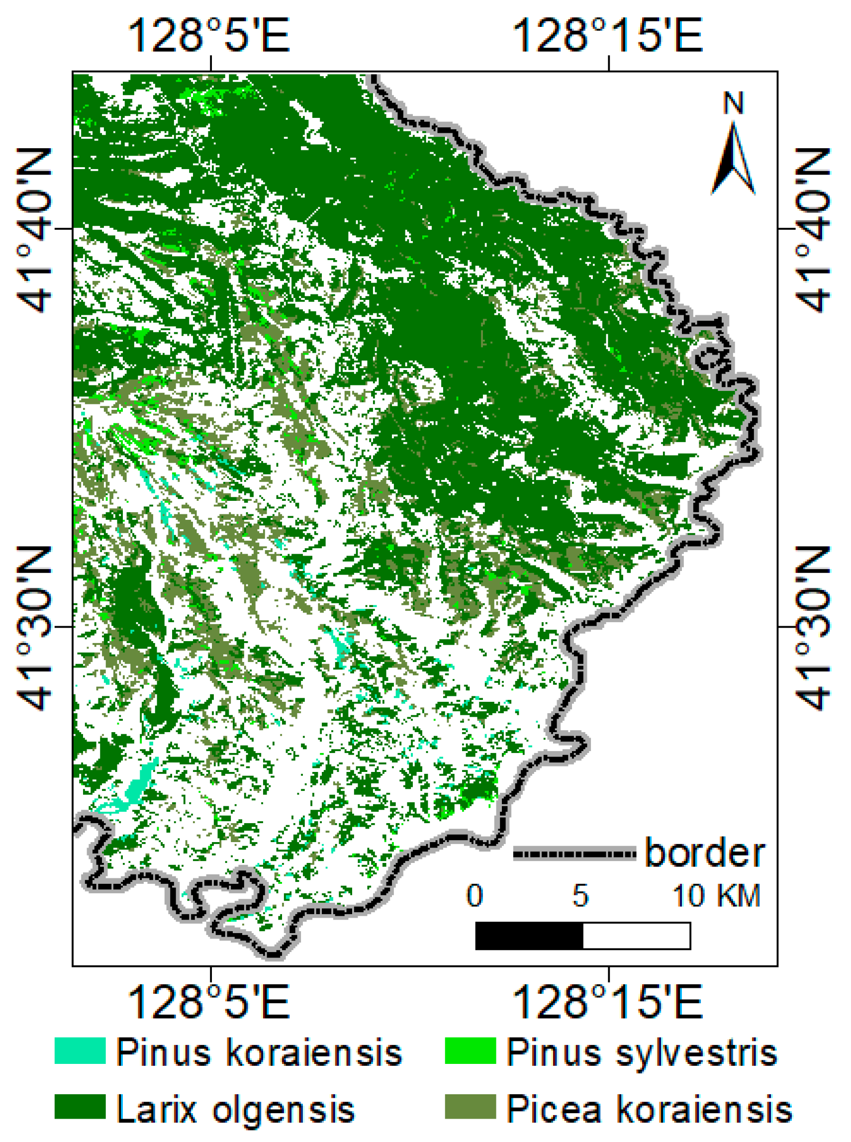
2.1. Study Area
2.2. Data Sources and Preprocessing
2.3. Distribution of Forest Types Based on CD-CNN-CRF
2.4. Leaf Area Index and Degree of Disaster
- (1)
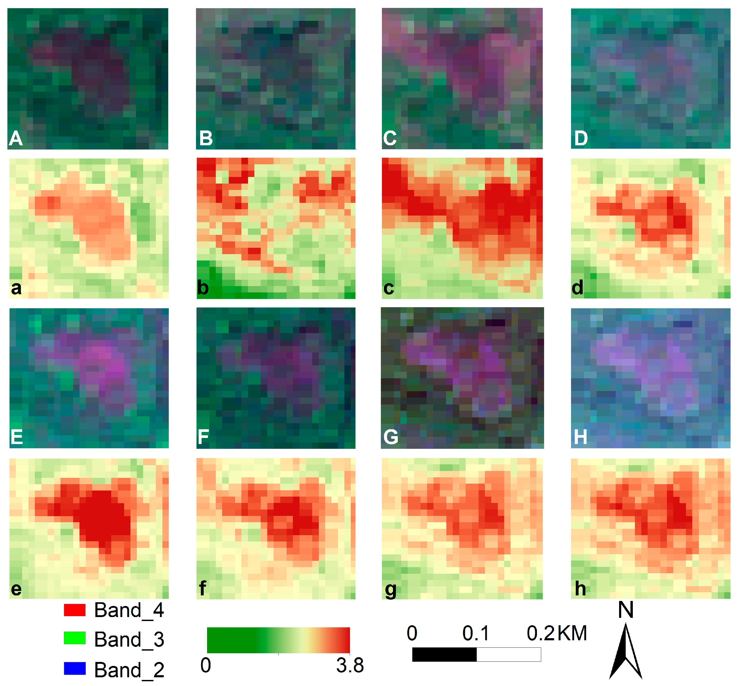
- Leaf Area Index Extraction
- (2)
- Division of Disaster Stage
- (3)
- Disaster Severity Calculation Based on Defoliation Rate
2.5. Analysis of Influencing Factors Based on the Geographical Detector
2.6. Technical Route Introduction
3. Results
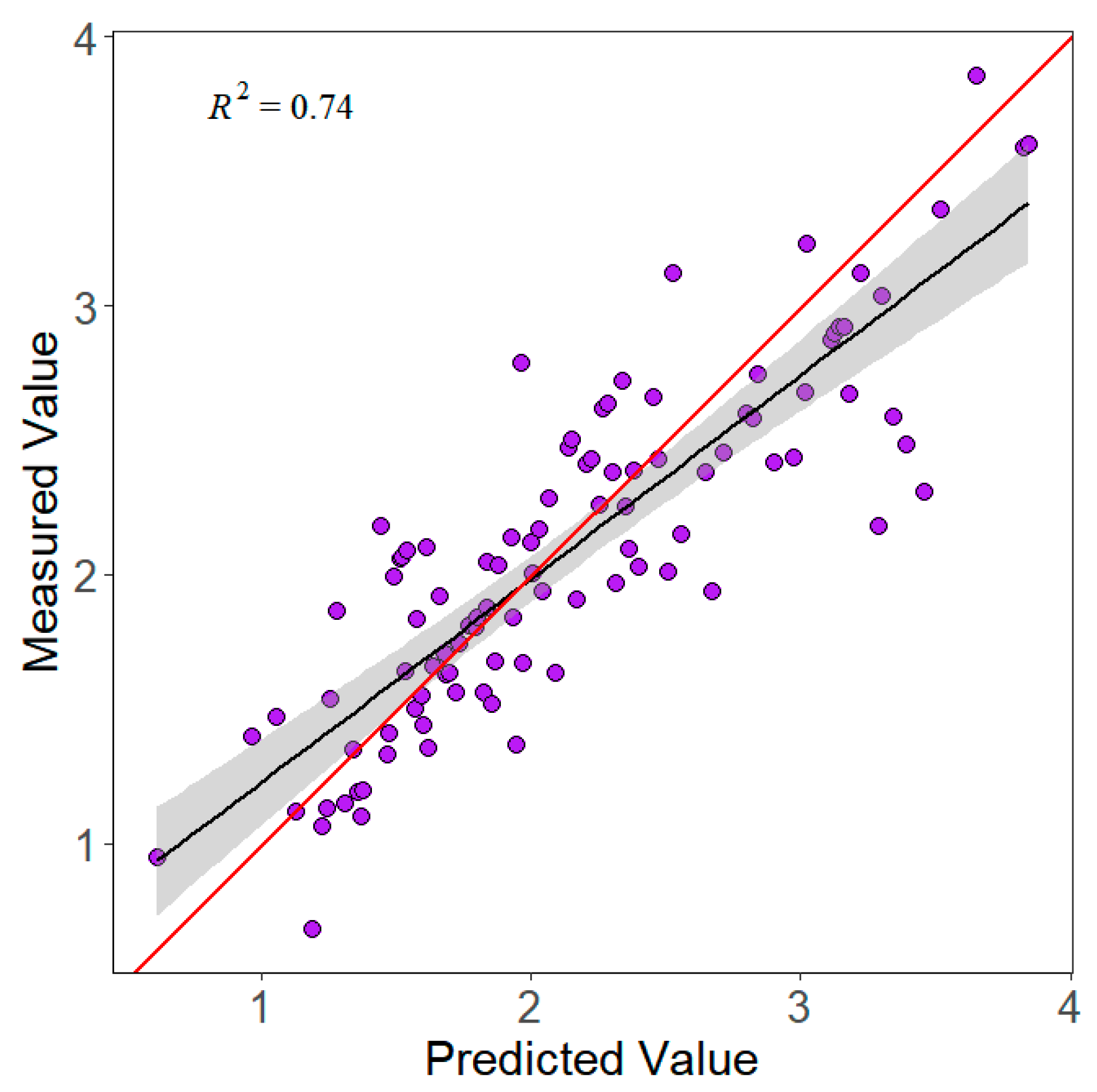
3.1. Forest-Type Classification and LAI Inversion
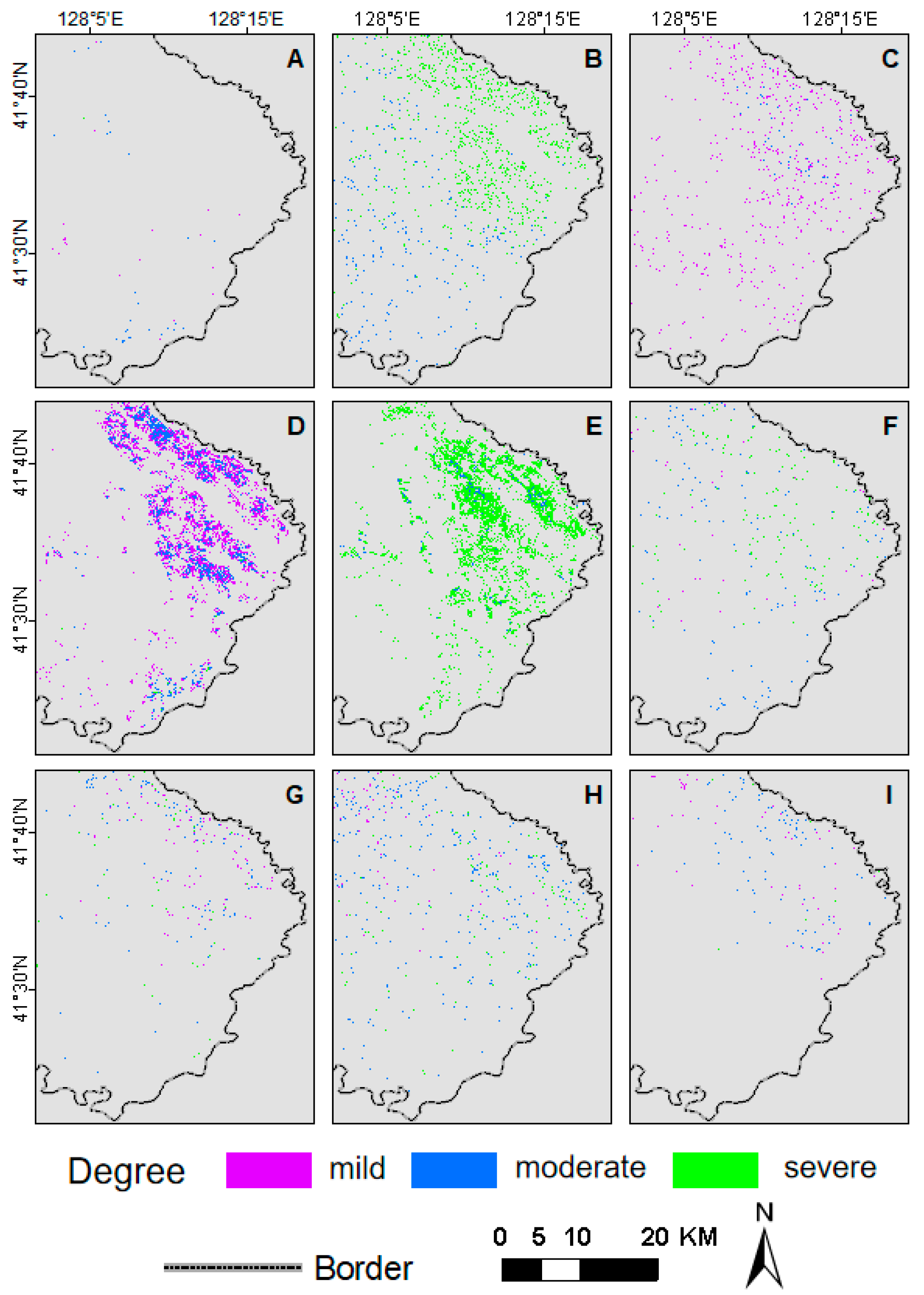
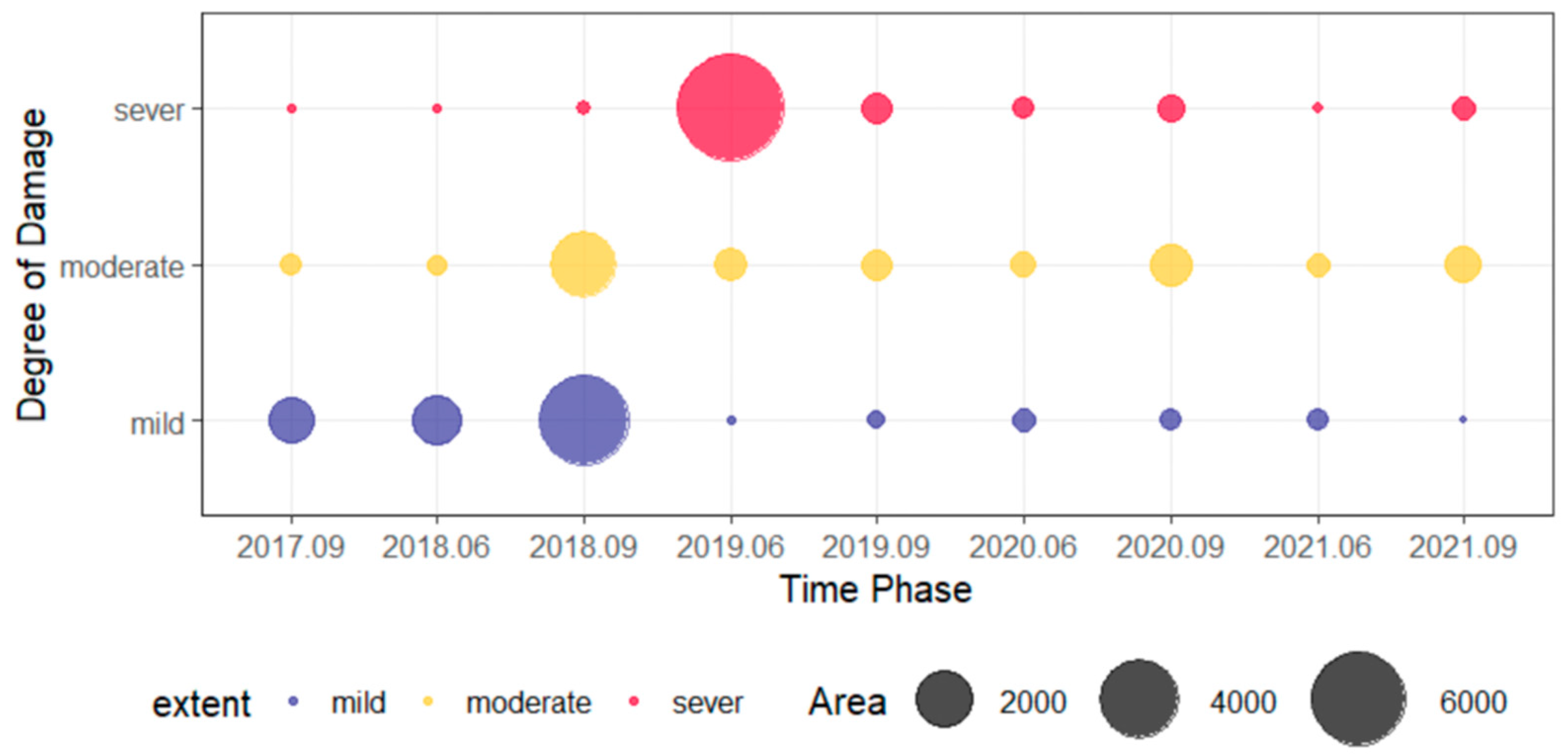
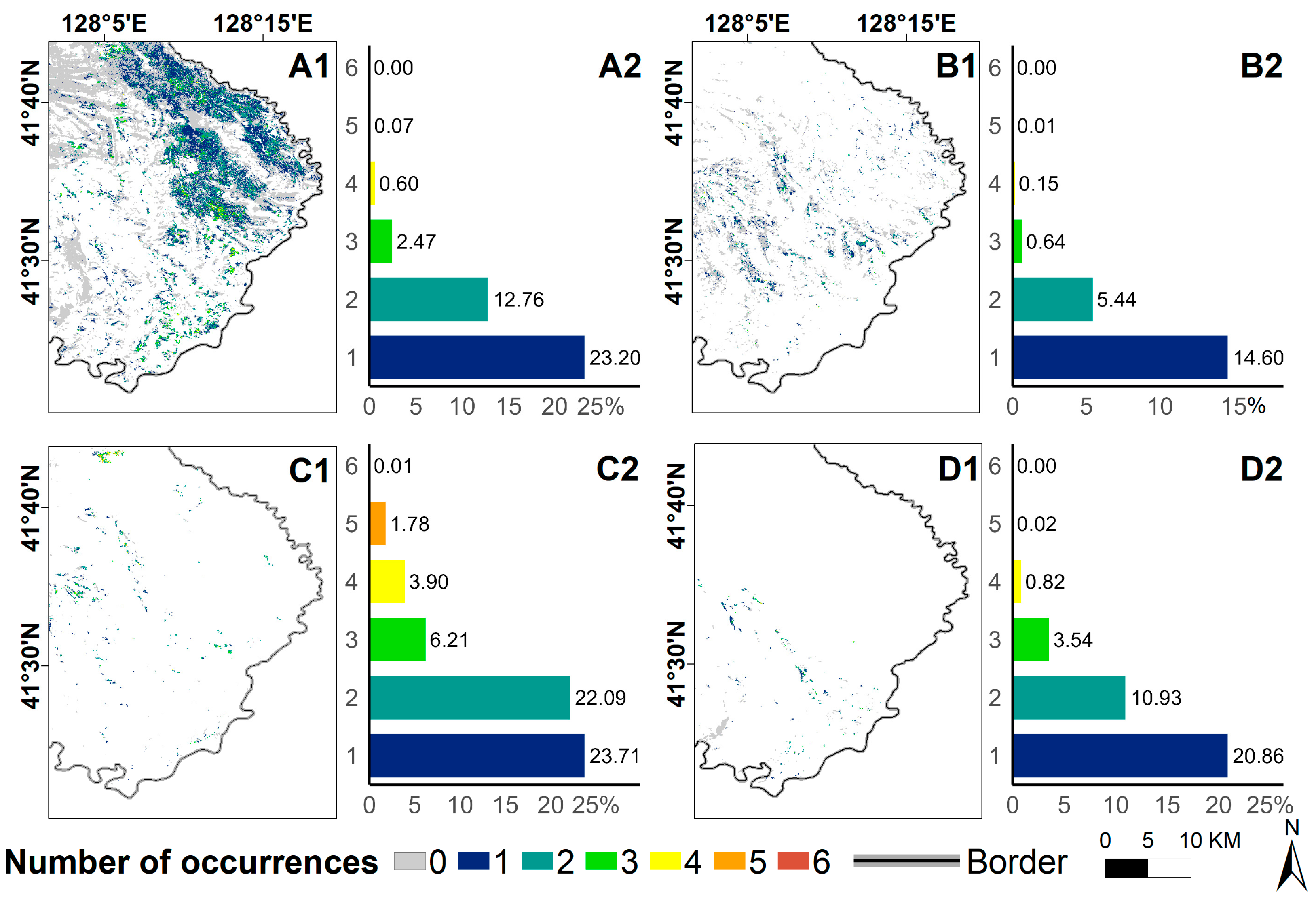
3.2. Evolution of the Spatiotemporal Pattern of Forest Defoliating Pest Disasters
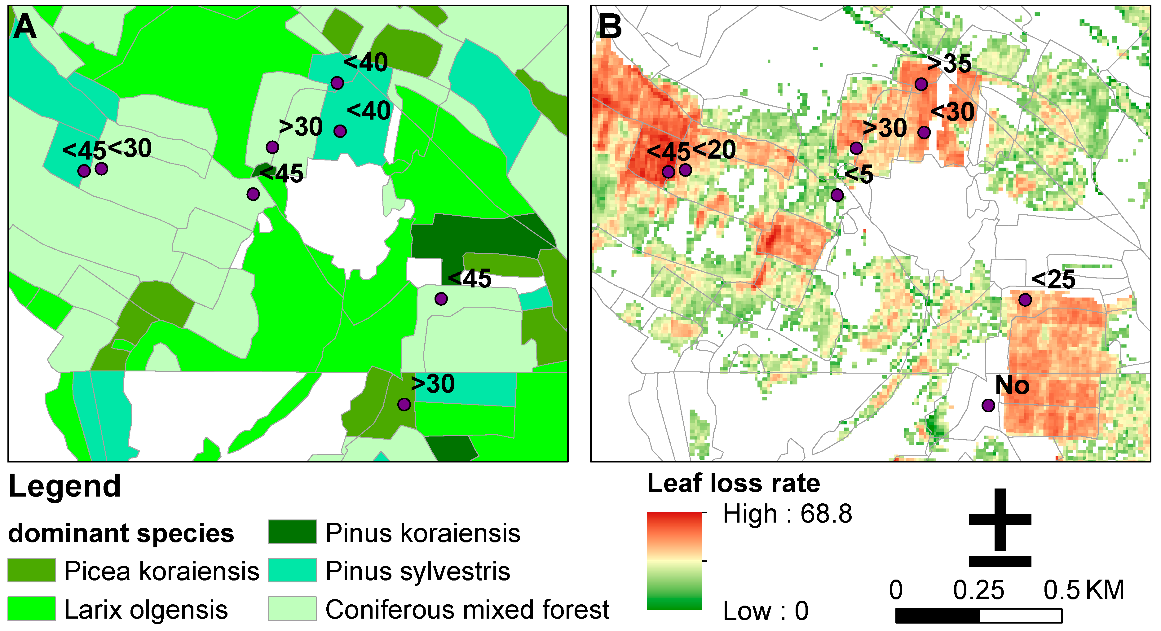
3.3. Differences in Disaster Characteristics among Different Forest Types
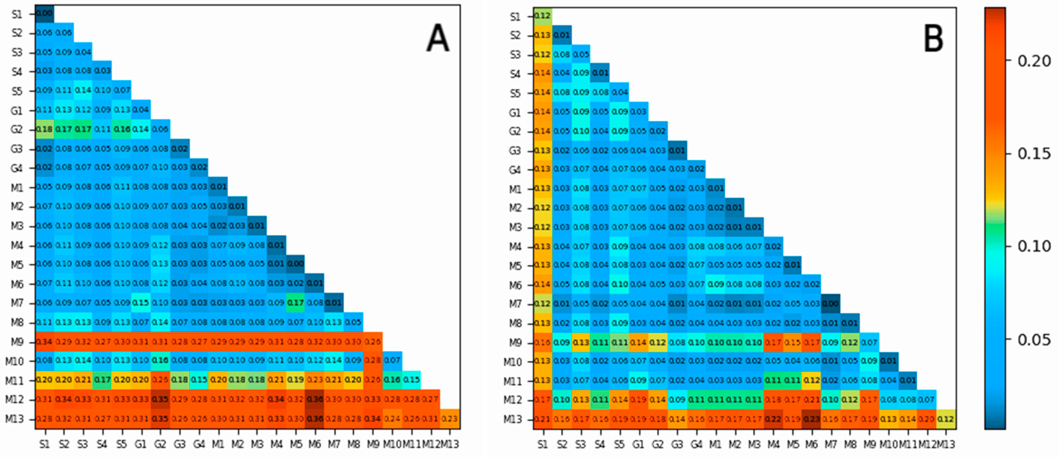
3.4. Driving Factors and Their Interactions in Different Forest Types
4. Discussion
4.1. Spatiotemporal Pattern Evolution
4.2. Driving Factors of Pine Caterpillar Disasters
4.3. Significance and Limitations
5. Research Conclusions
Author Contributions
Funding
Data Availability Statement
Conflicts of Interest
Appendix A


| Type | Area (ha) | Patches Number | Average Area of Patches (ha) | Proportion (%) | Mapping Accuracy (%) | User Accuracy (%) |
|---|---|---|---|---|---|---|
| Larix olgensis | 35,987.90 | 1356 | 26.54 | 31.81 | 91.13 | 95.44 |
| Picea koraiensis | 10,901.37 | 1910 | 5.71 | 9.64 | 89.26 | 93.46 |
| Pinus sylvestris var. mongolica | 1320.22 | 522 | 2.53 | 1.17 | 88.77 | 89.91 |
| Pinus koraiensis | 829.15 | 248 | 3.34 | 0.73 | 94.29 | 97.67 |
| Minimum | Maximum | Average | Standard Deviation | <0 | >0 | ||
|---|---|---|---|---|---|---|---|
| Full Phase | Larix olgensis | −0.11 | 0.39 | 0.10 | 0.03 | 204.26 | 35,783.64 |
| Picea koraiensis | −0.05 | 0.41 | 0.14 | 0.05 | 11.22 | 10,890.15 | |
| Pinus sylvestris | −0.11 | 0.36 | 0.06 | 0.04 | 92.04 | 1228.18 | |
| Pinus koraiensis | −0.05 | 0.39 | 0.10 | 0.07 | 7.39 | 821.76 | |
| Developing Phase | Larix olgensis | −0.97 | 1.21 | 0.10 | 0.24 | 13,835.35 | 22,152.55 |
| Picea koraiensis | −0.90 | 1.22 | 0.21 | 0.17 | 974.53 | 9926.84 | |
| Pinus sylvestris | −0.56 | 0.83 | 0.14 | 0.14 | 155.43 | 1164.79 | |
| Pinus koraiensis | −1.00 | 1.05 | 0.18 | 0.15 | 61.25 | 767.90 | |
| Stationary Phase | Larix olgensis | −0.40 | 1.49 | 0.15 | 0.18 | 6285.40 | 29,702.50 |
| Picea koraiensis | −0.40 | 1.42 | 0.12 | 0.19 | 2678.28 | 8223.09 | |
| Pinus sylvestris | −0.40 | 0.94 | −0.06 | 0.16 | 857.30 | 462.92 | |
| Pinus koraiensis | −0.40 | 1.11 | 0.04 | 0.20 | 369.71 | 459.44 |
| S1 | S2 | S3 | S4 | S5 | G1 | G2 | G3 | G4 | M1 | M2 | M3 | M4 | M5 | M6 | M7 | M8 | M9 | M10 | M11 | ||
|---|---|---|---|---|---|---|---|---|---|---|---|---|---|---|---|---|---|---|---|---|---|
| Pinus sylvestris | A | 0.0982 | 0.0735 | 0.0585 | 0.0157 | 0.0762 | 0.2196 | 0.0255 | 0.0245 | 0.02 | 0.0645 | 0.0342 | 0.0357 | 0.1044 | 0.1131 | 0.1178 | 0.0694 | 0.1995 | 0.0474 | 0.1042 | 0.1068 |
| *** | *** | *** | *** | *** | *** | * | *** | ** | * | *** | *** | *** | *** | *** | *** | *** | *** | ||||
| B | 0.0006 | 0.0083 | 0.0064 | 0.0013 | 0.0026 | 0.0008 | 0.0005 | 0.0031 | 0.0007 | 0.0015 | 0.0019 | 0.0013 | 0.0042 | 0.0018 | 0.0047 | 0.0005 | 0.0012 | 0.0011 | 0.0016 | 0.0063 | |
| ** | * | *** | * | *** | *** | *** | ** | * | ** | *** | *** | *** | *** | *** | |||||||
| Picea koraiensis | A | 0.0009 | 0.0483 | 0.0237 | 0.0305 | 0.0339 | 0.019 | 0.0423 | 0.0075 | 0.0404 | 0.0254 | 0.023 | 0.0326 | 0.0037 | 0.0125 | 0.0045 | 0.0088 | 0.026 | 0.1021 | 0.0569 | 0.0682 |
| *** | *** | *** | *** | *** | *** | *** | *** | *** | *** | *** | *** | ** | *** | *** | *** | *** | *** | ||||
| B | 0.0003 | 0.0003 | 0.015 | 0.0005 | 0.0148 | 0 | 0.0039 | 0.0018 | 0.001 | 0.0012 | 0.0008 | 0.0008 | 0 | 0.0002 | 0 | 0.0055 | 0.0003 | 0.0026 | 0.0001 | 0.0009 | |
| *** | *** | *** | *** | *** | *** | *** | * | *** | *** | *** | |||||||||||
| Larix olgensis | A | 0.0013 | 0.0222 | 0.0375 | 0.0121 | 0.0619 | 0.0558 | 0.1221 | 0.0281 | 0.0182 | 0.0099 | 0.0136 | 0.0072 | 0.0201 | 0.0094 | 0.0286 | 0.0121 | 0.0698 | 0.3207 | 0.0918 | 0.1754 |
| B | 0 | 0.0002 | 0.0004 | 0.0001 | 0.0005 | 0 | 0.0005 | 0.0001 | 0 | 0.0002 | 0.0008 | 0.0005 | 0.0002 | 0.0002 | 0.0006 | 0.0005 | 0 | 0.0003 | 0.0001 | 0.0003 | |
| ** | * | * | * | * | ** | ** | * | * | * | * | * | * | * | * | * | * | * | ||||
| Pinus koraiensis | A | 0.097 | 0.098 | 0.0293 | 0.0395 | 0.1002 | 0.1021 | 0.1646 | 0.0151 | 0.0003 | 0.1199 | 0.1244 | 0.1244 | 0.0391 | 0.0254 | 0.0556 | 0.0482 | 0.04 | 0.0501 | 0.0143 | 0.0443 |
| *** | *** | * | *** | * | *** | *** | * | *** | *** | *** | * | * | *** | * | *** | * | * | ||||
| B | 0.0001 | 0.0067 | 0.0107 | 0.0014 | 0.0171 | 0.0066 | 0.0041 | 0.006 | 0.002 | 0.0106 | 0.0094 | 0.0094 | 0.0032 | 0.0033 | 0.0038 | 0.0032 | 0.0027 | 0.0006 | 0.0006 | 0.0051 | |
| *** | ** | ** | * |
References
- Kautz, M.; Meddens, A.J.H.; Hall, R.J.; Arneth, A. Biotic disturbances in Northern Hemisphere forests—A synthesis of recent data, uncertainties and implications for forest monitoring and modelling. Glob. Ecol. Biogeogr. 2017, 26, 533–552. [Google Scholar] [CrossRef]
- Stewart, D.; Djoumad, A.; Holden, D.; Kimoto, T.; Capron, A.; Dubatolov, V.V.; Akhanaev, Y.B.; Yakimova, M.E.; Martemyanov, V.V.; Cusson, M. A TaqMan Assay for the Detection and Monitoring of Potentially Invasive Lasiocampids, with Particular Attention to the Siberian Silk Moth, Dendrolimus sibiricus (Lepidoptera: Lasiocampidae). J. Insect Sci. (Online) 2023, 23, 5. [Google Scholar] [CrossRef] [PubMed]
- Metsaranta, J.; Shaw, C.; Kurz, W.; Boisvenue, C.; Morken, S. Uncertainty of inventory-based estimates of the carbon dynamics of Canada’s managed forest (1990–2014). Can. J. For. Res. 2017, 47, 1082–1094. [Google Scholar] [CrossRef]
- Medvigy, D.; Clark, K.L.; Skowronski, N.S.; Schäfer, K.V.R. Simulated impacts of insect defoliation on forest carbon dynamics. Environ. Res. Lett. 2012, 7, 045703. [Google Scholar] [CrossRef]
- Pasqualotto, N.; D’Urso, G.; Bolognesi, S.F.; Belfiore, O.R.; Wittenberghe, S.V.; Delegido, J.; Pezzola, A.; Winschel, C.; Moreno, J. Retrieval of Evapotranspiration from Sentinel-2: Comparison of Vegetation Indices, Semi-Empirical Models and SNAP Biophysical Processor Approach. Agronomy 2019, 9, 663. [Google Scholar] [CrossRef]
- Soukhovolsky, V.; Krasnoperova, P.; Kovalev, A.; Sviderskaya, I.; Tarasova, O.; Ivanova, Y.; Akhanaev, Y.; Martemyanov, V. Differentiation of Forest Stands by Susceptibility to Folivores: A Retrospective Analysis of Time Series of Annual Tree Rings with Application of the Fluctuation-Dissipation Theorem. Forests 2023, 14, 1385. [Google Scholar] [CrossRef]
- Campbell, M.J.; Williams, J.P.; Berryman, E.M. Using Remote Sensing and Climate Data to Map the Extent and Severity of Balsam Woolly Adelgid Infestation in Northern Utah, USA. Forests 2023, 14, 1357. [Google Scholar] [CrossRef]
- Liu, Y.; Zhan, Z.; Ren, L.; Ze, S.; Yu, L.; Jiang, Q.; Luo, Y. Hyperspectral evidence of early-stage pine shoot beetle attack in Yunnan pine. For. Ecol. Manag. 2021, 497, 119505. [Google Scholar] [CrossRef]
- Huang, Z.; Zhang, Y. Remote sensing of spruce budworm defoliation using EO-1 Hyperion hyperspectral data: An example in Quebec, Canada. IOP Conf. Ser. Earth Environ. Sci. 2016, 34, 012017. [Google Scholar] [CrossRef]
- Jha, P.K.; Zhang, N.; Rijal, J.P.; Parker, L.E.; Ostoja, S.; Pathak, T.B. Climate change impacts on insect pests for high value specialty crops in California. Sci. Total Environ. 2023, 906, 167605. [Google Scholar] [CrossRef]
- Pasquarella, V.J.; Bradley, B.A.; Woodcock, C.E. Near-Real-Time Monitoring of Insect Defoliation Using Landsat Time Series. Forests 2017, 8, 275. [Google Scholar] [CrossRef]
- Hall, R.J.; Castilla, G.; White, J.C.; Cooke, B.J.; Skakun, R.S. Remote sensing of forest pest damage: A review and lessons learned from a Canadian perspective. Can. Entomol. 2016, 148, S296–S356. [Google Scholar] [CrossRef]
- Zhu, Z.; Woodcock, C.E.; Olofsson, P. Continuous monitoring of forest disturbance using all available Landsat imagery. Remote Sens. Environ. 2012, 122, 75–91. [Google Scholar] [CrossRef]
- Pastick, N.J.; Jorgenson, M.T.; Goetz, S.J.; Jones, B.M.; Wylie, B.K.; Minsley, B.J.; Genet, H.; Knight, J.F.; Swanson, D.K.; Jorgenson, J.C. Spatiotemporal remote sensing of ecosystem change and causation across Alaska. Glob. Change Biol. 2018, 25, 1171–1189. [Google Scholar] [CrossRef] [PubMed]
- Yu, L.; Zhan, Z.; Ren, L.; Zong, S.; Luo, Y.; Huang, H. Evaluating the Potential of WorldView-3 Data to Classify Different Shoot Damage Ratios of Pinus yunnanensis. Forests 2020, 11, 417. [Google Scholar] [CrossRef]
- Abolfazl, J.; Mahdi, P.; Davood, M.-G.; Omid, R.; Himan, S.; Ataollah, S.; Saro, L.; Tien, B.D.; Biswajeet, P. Swarm intelligence optimization of the group method of data handling using the cuckoo search and whale optimization algorithms to model and predict landslides. Appl. Soft Comput. J. 2022, 116, 108254. [Google Scholar]
- Sathish, C.; Nakhawa, A.D.; Bharti, V.S.; Jaiswar, A.K.; Deshmukhe, G. Estimation of extent of the mangrove defoliation caused by insect Hyblaea puera (Cramer, 1777) around Dharamtar creek, India using Sentinel 2 images. Reg. Stud. Mar. Sci. 2021, 48, 102054. [Google Scholar] [CrossRef]
- Fang, L.; Yu, Y.; Fang, G.; Zhang, X.; Yu, Z.; Zhang, X.; Crocker, E.; Yang, J. Effects of meteorological factors on the defoliation dynamics of the larch caterpillar (Dendrolimus superans Butler) in the Great Xing’an boreal forests. J. For. Res. 2021, 32, 2683–2697. [Google Scholar] [CrossRef]
- Damestoy, T.; Jactel, H.; Belouard, T.; Schmuck, H.; Plomion, C.; Castagneyrol, B. Tree species identity and forest composition affect the number of oak processionary moth captured in pheromone traps and the intensity of larval defoliation. Agric. For. Entomol. 2020, 22, 169–177. [Google Scholar] [CrossRef]
- Lombardero, M.J.; Ayres, M.P.; Bonello, P.; Cipollini, D.; Herms, D.A. Effects of defoliation and site quality on growth and defenses of Pinus pinaster and P. radiata. For. Ecol. Manag. 2016, 382, 39–50. [Google Scholar] [CrossRef]
- Ali, A.M.; Abdullah, H.; Darvishzadeh, R.; Skidmore, A.K.; Heurich, M.; Roeoesli, C.; Paganini, M.; Heiden, U.; Marshall, D. Canopy Chlorophyll Content Retrieved from Time Series Remote Sensing Data as a Proxy for Detecting Bark Beetle Infestation. Remote Sens. Appl. Soc. Environ. 2021, 22, 100524. [Google Scholar] [CrossRef]
- Sánchez-Cuesta, R.; Ruiz-Gómez, F.J.; Duque-Lazo, J.; González-Moreno, P.; Navarro-Cerrillo, R.M. The environmental drivers influencing spatio-temporal dynamics of oak defoliation and mortality in dehesas of Southern Spain. For. Ecol. Manag. 2021, 485, 118946. [Google Scholar] [CrossRef]
- Bao, Y.; Na, L.; Han, A.; Guna, A.; Wang, F.; Liu, X.; Zhang, J.; Wang, C.; Tong, S.; Bao, Y. Drought drives the pine caterpillars (Dendrolimus spp.) outbreaks and their prediction under different RCPs scenarios: A case study of Shandong Province, China. For. Ecol. Manag. 2020, 475, 118446. [Google Scholar] [CrossRef]
- Zhang, B.; Leroux, S.J.; Bowden, J.J.; Hargan, K.E.; Hurford, A.; Moise, E.R. Species distribution model identifies influence of climatic constraints on severe defoliation at the leading edge of a native insect outbreak. For. Ecol. Manag. 2023, 544, 121166. [Google Scholar] [CrossRef]
- Charbonneau, D.; Lorenzetti, F.; Doyon, F.; Mauffette, Y. The influence of stand and landscape characteristics on forest tent caterpillar (Malacosoma disstria) defoliation dynamics: The case of the 1999–2002 outbreak in northwestern Quebec. Can. J. For. Res. 2012, 42, 1827–1836. [Google Scholar] [CrossRef]
- Liu, Y.; Huang, J.; Fang, G.; Sun, H.; Yin, Y.; Zhang, X. Fine-scale forest biological hazard in China show significant spatial and temporal heterogeneity. Ecol. Indic. 2022, 145, 109676. [Google Scholar] [CrossRef]
- Li, M.; MacLean, D.; Hennigar, C.; Ogilvie, J. Spatial-Temporal Patterns of Spruce Budworm Defoliation within Plots in Québec. Forests 2019, 10, 232. [Google Scholar] [CrossRef]
- Bae, S.; Müller, J.; Förster, B.; Hilmers, T.; Hochrein, S.; Jacobs, M.; Leroy, B.M.L.; Pretzsch, H.; Weisser, W.W.; Mitesser, O. Tracking the temporal dynamics of insect defoliation by high-resolution radar satellite data. Methods Ecol. Evol. 2021, 13, 121–132. [Google Scholar] [CrossRef]
- Hu, J. The Occurrence Characteristics and Control Strategies of Intermediate Pests. Int. J. Ecol. 2014, 3, 43–46. [Google Scholar] [CrossRef]
- Wood, B.J. Pest control in Malaysia’s perennial crops: A half century perspective tracking the pathway to integrated pest management. Integr. Pest Manag. Rev. 2002, 7, 173–190. [Google Scholar] [CrossRef]
- Fatemeh, T.; Giorgio, F.; Parviz, S.; Ebrahim, E.; Massimo, G.; Givskov, S.J. Variation among populations of Trichogramma euproctidis (Hymenoptera: Trichogrammatidae) revealed by life table parameters: Perspectives for biological control. J. Econ. Entomol. 2023, 116, 1119–1127. [Google Scholar]
- Boersma, N.; Boardman, L.; Gilbert, M.; Terblanche, J.S. Cold Treatment Enhances Low-temperature Flight Performance in False Codling Moth, Thaumatotibia leucotreta (Lepidoptera: Tortricidae)]. Agric. For. Entomol. 2019, 21, 243–251. [Google Scholar]
- Foga, S.; Scaramuzza, P.L.; Guo, S.; Zhu, Z.; Dilley, R.D.; Beckmann, T.; Schmidt, G.L.; Dwyer, J.L.; Hughes, M.J.; Laue, B. Cloud detection algorithm comparison and validation for operational Landsat data products. Remote Sens. Environ. 2017, 194, 379–390. [Google Scholar] [CrossRef]
- Zhao, H.; Zhang, H.X.; Cao, Q.J.; Sun, S.J.; Han, X.; Palaoag, T.D. Design and Development of Image Recognition Toolkit Based on Deep Learning. Int. J. Pattern Recognit. Artif. Intell. 2020, 35, 2159002. [Google Scholar] [CrossRef]
- Liu, T.; Bao, G.; Li, Z.; Zhu, R.; Bao, Y.; Zhang, Z. Forset Type Classification with Jilin-1GP Spectral Satellite Image Based on Three-dimension Convolution Neural Network. J. Anhui Agric. Sci. 2023, 51, 96–101+108. [Google Scholar]
- Kuusk, A.; Pisek, J.; Lang, M.; Märdla, S. Estimation of Gap Fraction and Foliage Clumping in Forest Canopies. Remote Sens. 2018, 10, 1153. [Google Scholar] [CrossRef]
- Cohrs, C.W.; Cook, R.L.; Gray, J.M.; Albaugh, T.J. Sentinel-2 Leaf Area Index Estimation for Pine Plantations in the Southeastern United States. Remote Sens. 2020, 12, 1406. [Google Scholar] [CrossRef]
- Kalamandeen, M.; Gulamhussein, I.; Castro, J.B.; Sothe, C.; Rogers, C.A.; Snider, J.; Gonsamo, A. Climate change and human footprint increase insect defoliation across central boreal forests of Canada. Front. Ecol. Evol. 2023, 11, 1293311. [Google Scholar] [CrossRef]
- Bao, G.; Liu, T.; Zhang, Z.; Ren, Z.; Zhai, C.; Ding, M.; Jiang, X. Remote Sensing Inversion of Effective Leaf Area Index of Four Coniferous Forest Types and Their Spatial Distribution Rule in Changbai Mountain. Sci. Silvae Sin. 2024, 60, 127–138. [Google Scholar]
- Hejný, I.; Wallin, J.; Bogdan, M. Weak pattern recovery for SLOPE and its robust versions. arXiv 2023, arXiv:2303.10970. [Google Scholar]
- Jiang, X.; Bao, G.; Zhai, C.; Liu, T.; Ren, Z.; Ding, M.; Zhang, W.; Du, Y. Study on Quantitative Inversion of Spatial Pattern of Forest Leaf Eating Pest Disaster. J. Southwest For. Univ. (Nat.) 2024, 44, 125–134. [Google Scholar]
- Wang, J.; Xu, C. Geographic detector: Principle and outlook. Acta Geogr. Sin. 2017, 72, 116–134. [Google Scholar]
- Liu, C.; Li, W.; Wang, W.; Zhou, H.; Liang, T.; Hou, F.; Xu, J.; Xue, P. Quantitative spatial analysis of vegetation dynamics and potential driving factors in a typical alpine region on the northeastern Tibetan Plateau using the Google Earth Engine. Catena 2021, 206, 105500. [Google Scholar] [CrossRef]
- Zhou, Q.; Zhang, X.; Yu, L.; Ren, L.; Luo, Y. Combining WV-2 images and tree physiological factors to detect damage stages of Populus gansuensis by Asian longhorned beetle (Anoplophora glabripennis) at the tree level. For. Ecosyst. 2021, 8, 479–490. [Google Scholar] [CrossRef]
- Bao, Y.; Han, A.; Zhang, J.; Liu, X.; Tong, Z.; Bao, Y. Contribution of the synergistic interaction between topography and climate variables to pine caterpillar (Dendrolimus spp.) outbreaks in Shandong Province, China. Agric. For. Meteorol. 2022, 322, 109023. [Google Scholar] [CrossRef]
- Zhang, N.; Wang, Y.; Zhang, X. Extraction of tree crowns damaged by Dendrolimus tabulaeformis Tsai et Liu via spectral-spatial classification using UAV-based hyperspectral images. Plant Methods 2020, 16, 135. [Google Scholar] [CrossRef]
- Nanninga, C.; Ward, S.F.; Aukema, B.H.; Montgomery, R.A. The effects of chilling and forcing temperatures on spring synchrony between larch casebearer and tamarack. Agric. For. Entomol. 2023, 25, 658–668. [Google Scholar] [CrossRef]
- Bai, Y.; Wong, C.P.; Jiang, B.; Hughes, A.C.; Wang, M.; Wang, Q. Developing China’s Ecological Redline Policy using ecosystem services assessments for land use planning. Nat. Commun. 2018, 9, 3034. [Google Scholar] [CrossRef]
- Michael, J.; Claude, B.; David, C.; Thierry, C.; Elisavet, C.; Katharina, D.-S.; Gianni, G.; Anton, J.M.J.; Alan, M.; Maria, N.N.; et al. Pest categorisation of Dendrolimus sibiricus. EFSA J. Eur. Food Saf. Auth. 2018, 16, e05301. [Google Scholar]
- Fatih, S.; Ece, Ö.G.; Korhan, E.; Emre, S.O. Comparative study of the analytical hierarchy process, frequency ratio, and logistic regression models for predicting the susceptibility to Ips sexdentatus in Crimean pine forests. Ecol. Inform. 2022, 71, 101811. [Google Scholar]
- Zhu, C.; Zhang, X.; Zhang, N.; Hassan, M.A.; Zhao, L. Assessing the Defoliation of Pine Forests in a Long Time-Series and Spatiotemporal Prediction of the Defoliation Using Landsat Data. Remote Sens. 2018, 10, 360. [Google Scholar] [CrossRef]
- Choi, W.I.; Nam, Y.; Lee, C.Y.; Choi, B.K.; Shin, Y.J.; Lim, J.-H.; Koh, S.-H.; Park, Y.-S. Changes in Major Insect Pests of Pine Forests in Korea Over the Last 50 Years. Forests 2019, 10, 692. [Google Scholar] [CrossRef]
- Ulf, B.; David, F.; Andrew, L.; Derek, J.; Marco, C.; Carlo, U.; Michael, G.; Kurt, N.; Tom, L.; Jan, E. Three centuries of insect outbreaks across the European Alps. New Phytol. 2009, 182, 929–941. [Google Scholar]
- Cen, C.; Parinaz, R.B.; Aaron, W. Assessing spatial and temporal dynamics of a spruce budworm outbreak across the complex forested landscape of Maine, USA. Ann. For. Sci. 2021, 78, 33. [Google Scholar]
- Toïgo, M.; Nicolas, M.; Jonard, M.; Croisé, L.; Nageleisen, L.-M.; Jactel, H. Temporal trends in tree defoliation and response to multiple biotic and abiotic stresses. For. Ecol. Manag. 2020, 477, 118476. [Google Scholar] [CrossRef]
- Anton, K.; Vladislav, S. Analysis of Forest Stand Resistance to Insect Attack According to Remote Sensing Data. Forests 2021, 12, 1188. [Google Scholar] [CrossRef]
- Zhang, N.; Zhang, X.; Yang, G.; Zhu, C.; Huo, L.; Feng, H. Assessment of defoliation during the D e ndrolimus tabulaeformis Tsai et Liu disaster outbreak using UAV-based hyperspectral images. Remote Sens. Environ. 2018, 217, 323–339. [Google Scholar] [CrossRef]
- Hua, H.; Wu, C.; Jassal, R.S.; Huang, J.; Liu, R.; Wang, Y. Pine caterpillar occurrence modeling using satellite spring phenology and meteorological variables. Environ. Res. Lett. 2022, 17, 104046. [Google Scholar] [CrossRef]
- Zhang, B.; MacLean, D.A.; Johns, R.C.; Eveleigh, E.S.; Edwards, S. Hardwood-softwood composition influences early-instar larval dispersal mortality during a spruce budworm outbreak. For. Ecol. Manag. 2020, 463, 118035. [Google Scholar] [CrossRef]
- Rouault, G.; Candau, J.-N.; Lieutier, F.; Nageleisen, L.-M.; Martin, J.-C.; Warzée, N. Effects of drought and heat on forest insect populations in relation to the 2003 drought in Western Europe. Ann. For. Sci. 2006, 63, 613–624. [Google Scholar] [CrossRef]
- Ece, Ö.G.; Fatih, S.; Emre, S.O.; Korhan, E. Determination of some factors leading to the infestation of Ips sexdentatus in crimean pine stands. For. Ecol. Manag. 2022, 519, 120316. [Google Scholar]
- Yu, X.; Zhou, H.; Luo, T. Spatial and temporal variations in insect-infested acorn fall in a Quercus liaotungensis forest in North China. Ecol. Res. 2003, 18, 155–164. [Google Scholar] [CrossRef]


| Data Type | Data Name | Spatial Resolution/Scale Bar | Time | Link |
|---|---|---|---|---|
| Remote sensing image | Sentinel 2A | 10 m | June and September, 2017–2021 | https://scihub.copernicus.eu, accessed on 8 July 2023 |
| Auxiliary data | Second-Class Forest Resource Survey Data | 1:10 | 2018 | |
| High-Resolution Remote Sensing Imagery | <1 m | September, 2018 | https://www.google.com/maps, accessed on 8 July 2023 | |
| Digital Elevation Model (DEM) | 10 m | 2018 | https://www.gis5g.com, accessed on 8 July 2023 | |
| Survey Data from the Forest Protection Department of the Forestry Bureau | 10 m | June, 2020 | ||
| Meteorological Data | 30 m | 2018–2020 | Dr. Bintao Liu’s team |
| Category | Code | Factor | Description | Reference Documentation |
|---|---|---|---|---|
| Forest Space Structure | S1 | Origin | The study area’s plantations are primarily monoculture pine forests with simple stand structures, low biodiversity, and limited natural predator control, often resulting in large-scale disasters. In contrast, natural forests, with their higher biodiversity and complex biological networks, have more stable ecosystems and enhanced self-regulatory potential, leading to less severe disasters. | [44] |
| S2 | Age of Stand | Middle-aged and young forests have a significantly higher occurrence probability than other age groups, likely due to their developing structure and increased vulnerability. | [8] | |
| S3 | DBH (Diameter at Breast Height) | The vigor of trees directly reflects the growth condition of the plants; better vigor results in stronger resistance to pests and diseases. | [44] | |
| S4 | Crown Density | Forests with low canopy densities suffer more from pest damage than those with dense canopies, which have lower temperatures and weaker light, conditions unfavorable for adult pine caterpillars. | [24] | |
| S5 | Stand Density | When stand density is high, it affects the canopy closure and light intensity, especially in the central area of the forest where light conditions are relatively weak. These conditions are unfavorable for adult pine caterpillars to fly, mate, and lay eggs, resulting in relatively lower occurrences of pine caterpillars. | [24] | |
| Geographical Factors | G1 | Elevation | Lower elevation areas are more susceptible to insect outbreaks due to human interference. | [45] |
| G2 | Slope | Pine caterpillar outbreaks are more severe on gentle slopes than on steep slopes at the same elevation. An increased slope enhances soil erosion, thereby increasing forest vulnerability, with the degree of slope directly proportional to its weakening effect. | [45] | |
| G3 | Aspect | The slope direction directly impacts microhabitat temperature and humidity, influencing the distribution of sun-loving and shade-tolerant forest types. Pine caterpillars generally occur more frequently on sunny slopes than shady ones, and more on western slopes than eastern ones. | [46] | |
| G4 | Land Type | The soil structure facilitates trees’ nutrient absorption, adjusting their sensitivity to insects. Some insects also overwinter in the soil as eggs or larvae. | [45] | |
| Meteorological Factors | M1/M2/M3 | Average Annual Temperature of 2018/2019/2020 | Annual temperature ranges reflect extreme seasonal temperatures and the sea and land’s influence on a region. Warmer temperatures enable pine caterpillar larvae to develop faster and achieve higher survival rates. | [16] |
| M4/M5/M6 | Minimum Winter Temperature in 2018/2019/2020 | Warmer winters and springs may initially increase the synchronicity between leaf fall and Larix olgensis, while extremely warm spring temperatures may reduce the survival rate from larvae to adulthood. | [47] | |
| M7/M8 | Average Monthly Precipitation in Spring 2018/Summer 2020 | Precipitation can affect the water content and vitality of host trees by changing atmospheric and soil moisture, and can mechanically damage eggs and hatched larvae. This may adversely affect adult mating and suppress pine caterpillar occurrences. | [45] | |
| M9/M10/M11 | Sunshine in 2018/2019/2020 | Increased sunlight duration during the growing season enables insects to grow rapidly. | [45] | |
| M12/M13 | Relative Humidity in 2018/2019 | Extreme variations in relative humidity may affect the hatching process of eggs and subsequent survival rates, and may exacerbate the spread of pathogens. | [16] |
| Time | Low Humidity (0%–27%) | Moderate Humidity (27%–30%) | High Humidity (30%–100%) |
|---|---|---|---|
| 2017.09 | 76.01 | 23.98 | 0.01 |
| 2018.06 | 85.31 | 12.17 | 2.52 |
| 2018.09 | 87.54 | 9.05 | 3.41 |
| 2019.06 | 65.06 | 25.4 | 9.54 |
| 2019.09 | 93.08 | 6.49 | 0.43 |
| 2020.06 | 66.13 | 26.23 | 7.64 |
| 2020.09 | 61.17 | 26.82 | 12.01 |
| 2021.06 | 64.97 | 22.97 | 12.06 |
| 2021.09 | 74.47 | 21.84 | 3.69 |
Disclaimer/Publisher’s Note: The statements, opinions and data contained in all publications are solely those of the individual author(s) and contributor(s) and not of MDPI and/or the editor(s). MDPI and/or the editor(s) disclaim responsibility for any injury to people or property resulting from any ideas, methods, instructions or products referred to in the content. |
© 2024 by the authors. Licensee MDPI, Basel, Switzerland. This article is an open access article distributed under the terms and conditions of the Creative Commons Attribution (CC BY) license (https://creativecommons.org/licenses/by/4.0/).
Share and Cite
Jiang, X.; Liu, T.; Ding, M.; Zhang, W.; Zhai, C.; Lu, J.; He, H.; Luo, Y.; Bao, G.; Ren, Z. Changes in Spatiotemporal Pattern and Its Driving Factors of Suburban Forest Defoliating Pest Disasters. Forests 2024, 15, 1650. https://doi.org/10.3390/f15091650
Jiang X, Liu T, Ding M, Zhang W, Zhai C, Lu J, He H, Luo Y, Bao G, Ren Z. Changes in Spatiotemporal Pattern and Its Driving Factors of Suburban Forest Defoliating Pest Disasters. Forests. 2024; 15(9):1650. https://doi.org/10.3390/f15091650
Chicago/Turabian StyleJiang, Xuefei, Ting Liu, Mingming Ding, Wei Zhang, Chang Zhai, Junyan Lu, Huaijiang He, Ye Luo, Guangdao Bao, and Zhibin Ren. 2024. "Changes in Spatiotemporal Pattern and Its Driving Factors of Suburban Forest Defoliating Pest Disasters" Forests 15, no. 9: 1650. https://doi.org/10.3390/f15091650