Developing a Quality Assessment Index System for Scenic Forest Management: A Case Study from Xishan Mountain, Suburban Beijing

Abstract

The public’s demand for more and better forest landscapes is increasing as scenic forest tours flourish in China, especially in the capital, Beijing. How to improve the quality of scenic forests has become one of the greatest concerns of urban foresters. Although numerous studies have focused on scenic forest management, to date, no reports have been found on developing a quality assessment index system for scenic forest assessment. In this study, a simple and scientific index system was established using an analytical hierarchy process (AHP) to quantitatively assess scenic forest quality. The index system is composed of four scales: individual tree landscape quality, in-forest landscape quality, near-view forest landscape quality and far-view landscape quality. The in-forest landscape quality was determined by horizontal and vertical stand structures, species composition and under-canopy landscape traits. Near-view forest landscape quality was mainly determined by patch characteristics, seasonal change, visibility, color change of patches and stand age class. To test the validity of our quality assessment index system, scenic forests in Xishan were used as a case study. The results show that near-view forest landscape was the most important scale for the overall quality of the scenic forest, according to the priorities of the criterion layer, and the second most important scale was far-view forest landscape. Seasonal change, patch color contrast, patch distribution and patch shape accounted for 52.2% of the total of 13 indices in the near-view forest landscape. The integrated quality of scenic forests in Xishan was at an average level, and the in-forest landscape, near-view landscape and far-view landscape had below average quality.

1. Introduction

In general, scenic forests have high aesthetic values, especially the visual perception of beauty [1]. Currently, scenic forests, as popular travel attractions, play an increasingly important role in the pursuit of leisure for Chinese people. For instance, the highest number of daily visitors to Xiangshan Park, the most well-known scenic forest in Beijing, reached 138,000 on October 28, 2012, making this the best record since 1989 when the first “Red Leaf Festival” was launched [2]. Although the rush of tourism into scenic forests has triggered a series of ecological and social problems, it has also stimulated a new demand from the public for more and better forest landscapes [3]. Since 1985, more than 2400 forest parks have been established in China. However, most scenic forests, especially those in suburban areas in northern China, are derived from planted forests, which are comprised of few tree species, high stock density with mass self-pruning and low rates of natural generation due to poor light conditions [4]. In suburban Beijing, planted Pinus tabulaeformis Carr. and Platycladus orientalis (L.) Franco forests account for 39% of the total forest area, of which the young and middle-aged trees account for 87%. Hence, on the recommendation of urban foresters, the Chinese government reached a consensus that improving the quality of scenic forests should be given high priority [5]. For decades in China, management techniques for scenic forests, such as refilling [6], mixing [7], tending [8,9,10,11] and modulation of stock density [3], have been intensively studied. These techniques have been integrated based on the relationships between one or several stand structural factors and scenic beauty evaluation values of in-forest landscapes or near-view forest landscapes. Most measures of these techniques come from commercial forest management, because valid, systematic and scientific criteria for assessing the quality of scenic forests have not yet been established. Therefore, to evaluate the quality and to identify the problems of scenic forests for further improvement, establishing a quality assessment index system has become an issue of some urgency.

Landscape assessment addresses the quality of objective visual landscapes in terms of individual or social preferences for various landscape types, which is considered to be the key part in studies of landscape aesthetics and is the basis for landscape management, as well [12]. Assessments are based on the assumption that the scenic beauty of the entire landscape can be explained in terms of the aggregation of the values of landscape components [13]. For example, scenic forests, as a synthesis of structures, functions and aesthetics, have a large number of ecological, silvicultural and aesthetic components that affect their visual quality, such as tree height, crown size, species composition, tree density, color, crown patches, texture, patterns and shapes [14]. The structured method of landscape assessment describes, classifies, analyzes and then evaluates these components [12].

A number of methods in landscape assessment have been devised since the 1960s; they started with descriptive inventories based on the experience of experts who gradually turned to the public, the best source of data in their opinion. Public preference methods, such as SBE (scenic beauty estimation), consist of two approaches: quantitative public preference surveys and landscape features. These approaches became very popular. Today, given the development of geographic information systems (GIS), there is a trend to carry out visual landscape research using computer technology and digital data [15]. For the experts who assume that scenic quality is directly related to landscape diversity or variety, descriptive inventories are much simpler and more valid methods [5,16,17,18], in contrast with those approaches that involve public preferences and require massive surveys and measurements [19,20,21], while quantitative holistic methods rely on high-resolution DEM or digital aerial images [13,22]. In general, descriptive inventories, public preference models and quantitative holistic methods are the most popular methods of landscape assessment, and they greatly contribute to decision making and landscape management [23].

Although a number of studies have been carried out on scenic forests in China, a valid quality assessment system or a quality criterion has not been proposed to date. To grade the quality of scenic forests and help improve their visual quality, it is necessary to develop a scientific and systematic assessment index system. Based on research by Zhang [3], who analyzed scenic forest quality factors using principal components analysis (PCA), we have built a quality assessment index system using an analytical hierarchy process (AHP) through descriptive inventories, which are based on subjectively selected methods, but which can be applied objectively.

2. Study Area

2.1. Beijing and the Xishan Mountain Area

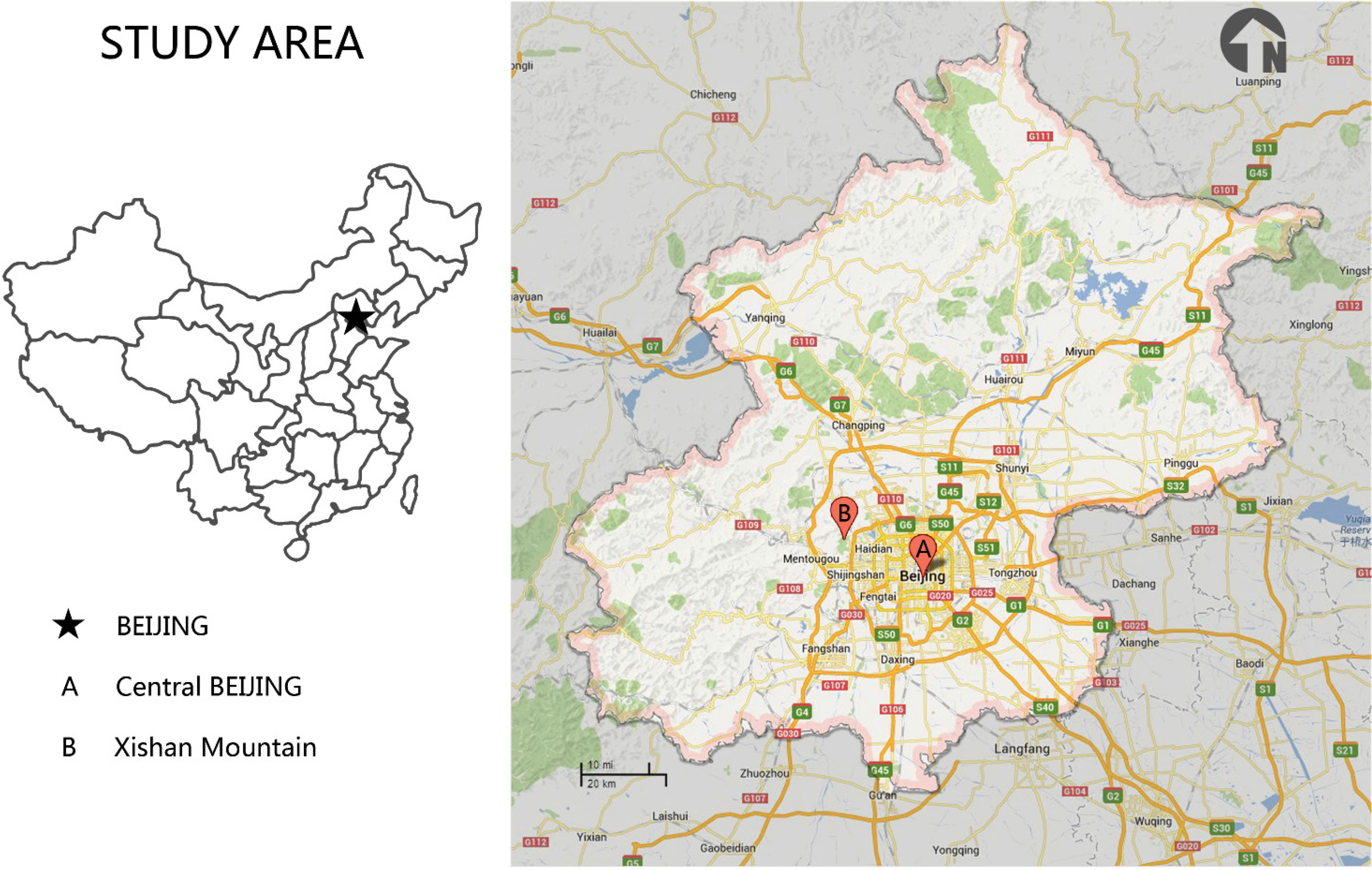
Beijing is located in the North China Plain, between 115°25′–117°30′ E longitude and 39°28′–41°05′ N latitude. The Taihang Mountains are to the west, and the Yanshan Mountains are to the northeast. The total mountainous area is 10,400 km², which accounts for 62% of the Beijing area. The mountains surround the central city and form an important natural buffer and recreational area.

Xishan Mountain, which is located in western Beijing and belongs to the Taihang Mountain Range, has a total area of 3000 km². It includes a series of hills, for example, the West Ling, Baihua, Miaofeng and Jiulong hills, which are of great interest to tourists. Our study plots are in the Xishan experimental forest farm, which are managed by the Beijing Municipal Bureau of Landscape and Forestry and are representative of scenic forests (Figure 1).

Figure 1. Location of the study area (redrawn by the author from Google Maps).

Figure 1. Location of the study area (redrawn by the author from Google Maps).

2.2. Climate

Beijing has a typical semi-humid continental monsoon climate with four distinct seasons. The annual average temperature is 10 °C–12 °C. In the coldest month, the temperature is between –7 °C and –4 °C, and in the hottest month, the temperature is 25 °C–36 °C. Extreme temperatures include a low of –27.4 °C and a high of 42 °C. The annual average temperature of the lower mountain area is 10 °C, gradually dropping to 8 °C towards the west and north. The annual frost-free period is 180–200 days. The average annual rainfall is approximately 630 mm and is unevenly distributed. Up to 75% of the annual precipitation falls in the summer and is often heavy in July and August, but precipitation falls sparingly in winter and spring from December to March. The annual evaporation, which is as high as 1800–2000 mm, is about three-times the annual precipitation and is closely related to location and elevation. In general, evaporation is greater in the mountains and at low elevations than in the plains and high altitude areas.

2.3. Vegetation

The zonal vegetation in Beijing is a mixture of pine and oak forests, and Pinus tabulaeformis and Quercus variabilis BI. are the dominant species. However, at present, up to 70% of the forest vegetation consists of plantations established during the 1950s and 1960s [9]. Most plantations on Xishan Mountain consist of P. tabulaeformis, P. orientalis, Robinia pseudoacacia Linn., Q. variabilis, Cotinus coggygria Scop., Prunus davidiana Franch. and Prunus sibirica (L.) Lam. The dominant shrub species are Vitex negundo Linn., Myripnois dioica Bge., Deutzia grandiflora Bge. and Spiraea trilobata Linn.

3. Methods

In our study, a group of 25 experts in forestry, ecology and tour planning were invited to help in the decision making process. The experts were from seven different institutions (forestry universities, an academy of forestry and ecology research institutes), with forestry backgrounds that are directly or indirectly related to forest management activities. Our indices were derived from the literature, especially the research carried out by Zhang (2010) [3], which aimed at finding the intrinsic relationship of scenic forest quality factors by principal components analysis (PCA), based on measurement data from a total of 130 plots and a very large number of landscape photographs of the low mountain areas of Beijing. Given our expert survey, we modified the indices and constructed a quality index system using an analytical hierarchy process (AHP). In the end, we assessed the Xishan forest scene to test the validity of our quality index system.

3.1. Analytical Hierarchy Process

The AHP is a method of group decision-making. It provides a comprehensive and rational framework for structuring a decision problem [24] and is widely used in assessment system development [25,26,27,28,29]. It represents and qualifies all relevant elements, relates them to the overall goal and then evaluates alternative solutions. To generate priorities, we decomposed the decision into the following four steps, using the method developed by Saaty (2008) [30].

Step 1: Decompose the problem into a hierarchy of goal, criterion and alternatives.

Step 2: Evaluate the elements of the hierarchy by a pairwise comparison method.

Step 3: Obtain a numerical priority for each element of the hierarchy, allowing diverse and often incompatible elements to be compared in a rational and consistent way.

Step 4: Calculate the numerical priorities for each of the decision alternatives.

Each of our 25 experts received a questionnaire based on the 41 indices (Table 1). Sufficient information was provided to understand the scenic forests, forest management and indices. Then, the experts evaluated the elements of the hierarchy by comparing them pairwise using a 9-point scale to find their impact on the element above them in the hierarchy. The matrix of pairwise comparisons represented the intensities of their preferences between individual pairs of alternatives. In the end, we received feedback from all 25 experts, from which the judgment matrices were constructed, the geometric mean used to represent the average ratio and the weights associated with the quality evaluation indices for scenic forests calculated.

3.2. Determination of Index Contributions to Scenic Forest Quality

To quantitatively obtain the contribution of each index for grading scenic forest quality, we divided each index into several degrees, referred to as sub-items, evaluated the general scenic forest quality out of a total score of 100 and then computed the score of each index or sub-item according to their priorities as follows:

TD_k = PB_i × PC_j × PD_k

(1)

SE_kl = 100 × TD_k × WE_kl

(2)

where B, C, D, E refer to the criterion (Level B), sub-criterion (Level C), index (Level D) and sub-item layer, respectively, PB_i is the criterion B_i’s priority in Level B under the overall goal, PC_j is the sub-criterion C_j’s priority in Level C under criterion B_i, PD_k is the index D_k’s priority in Level D under sub-criterion C_j, TD_k is the contribution of each index to scenic forest quality, WE_kl is the sub-item E_kl’s weight in the sub-item layer under index D_k, SE_kl is the score of sub-item E_kl under index D_k and 100 is the total score of scenic forest quality. The ranges of i, j, k and l are as follows: i = 1, …, 4, j = 1, …, 5, k = 1, …, 41 and l = 1, …, 5.

3.3. Determination of Quality Grades

According to the SE_kl (the score of sub-item E_kl under index D_k), we calculated the maximum score, Max(SD_k), and the minimum score, Min(SD_k), of the index D_k, then we calculated the maximum score, Max(SB_i), and the minimum score, Max(SB_i), of the criterion B_i as follows:

$$Max(S{B}_i)={\displaystyle \sum }_{k=1}^{ \text{n}}Max(S{D}_k)$$

(3)

$$Min(S{B}_i)={\displaystyle \sum }_{k=1}^{ \text{n}}Min(S{D}_k)$$

(4)

i = 1, 2, 3 and 4 refer to the individual tree landscape, in-forest landscape, near-view forest landscape and far-view forest landscape, respectively. k refers to the number of indices under the criterion B_i. We then classified the scenic forest quality into five grades: excellent (Grade 1), very good (Grade 2), average (Grade 3), below average (Grade 4) and failing (Grade 5). The score ranges of the five grades are as follows:

Grade 1: [(MaxSB_i–MinSB_i) × 80% + MinSB_i, (MaxSB_i–MinSB_i) + MinSB_i)]

(5)

Grade 2: [(MaxSB_i–MinSB_i) × 60% + MinSB_i, (MaxSB_i–MinSB_i) × 80% + MinSB_i)]

(6)

Grade 3: [(MaxSB_i–MinSB_i) × 40% + MinSB_i, (MaxSB_i–MinSB_i) × 60% + MinSB_i)]

(7)

Grade 4: [(MaxSB_i–MinSB_i) × 20% + MinSB_i, (MaxSB_i–MinSB_i) × 40% + MinSB_i)]

(8)

Grade 5: [MinSB_i, (MaxSB_i–MinSB_i) × 20% + MinSB_i]

(9)

3.4. Field Investigation

To validate the quality assessment index system, we carried out a field investigation at the Xishan experimental forest farm. A representative sampling method was used. Twenty-two samples of individual trees, 121 samples of in-forest landscapes, 62 samples of near-view forest landscapes and 11 samples of far-view forest landscapes were investigated. This investigation was implemented in the typically planted P. tabulaeformis, P. orientalis pure forests and mixed coniferous and broadleaved forests, which are composed of P. tabulaeformis, Q. variabilis, P. orientalis, P. davidiana and R. pseudoacacia. The individual trees were the isolated or dominant trees in the scenic area. The in-forest sample areas were 20 m × 20 m for pure stands and 20 m × 30 m for plantations of mixed species. Stand information, including tree location, tree height, crown diameter, cover of understories, stock density and forest structures, was measured in detail. Simultaneously, following the tour route, we took a large number of landscape photographs of all of the plots at different visual scales (in-forest, near-view and far-view) to aid in index assignment and quality assessment.

4. Results

4.1. Quality Assessment Index System for AHP

Following the advice of the experts, we obtained 41 indices (Table 1). To improve the understanding of visual perception from the point of view of the tourists, we constructed a quality assessment index system in multiple scales, which linked the physical structure of the scenic forests to their aesthetic quality. In the following, we propose and discuss four scales for our system, i.e., that of the individual tree landscape, in-forest landscape, near-view forest landscape and far-view forest landscape (Table 1). The individual tree landscape refers to an isolated tree or the dominant tree in a stand, which is usually the largest and the most eye-catching one. The quality of the individual tree landscape primarily regards the beauty of plant morphology, while in-forest landscape refers to the forest community and its under-canopy landscapes, where recreational activities mostly take place. The appearance of a forest landscape represents the entire scenery of the forest, which is largely characterized by patch patterns and shows the beauty of forest forms, lines, colors and textures. To be more specific about the appearance of the forest landscape, we defined appearance as near-view and far-view forest landscapes based on a perceived distance of 500 m. For a near-view forest landscape, the visible distance between an observation point and the forest view is less than 500 m, where the features of individual trees and patches can both be identified. In the far-view forest landscapes, beyond the immediate 500 m distance and up to 3000 m from an observation point, the details of individual trees become vague, and the visual impact of patches is dominant.

Table 1. Hierarchy and priorities of indices for the assessment of scenic forest quality.

Level A Overall goal	Level B (priority) Criterion layer	Level C (priority) Sub-criterion layer	Level D (priority) Index layer
Quality of scenic forests in Beijing A	Individual tree landscape B1 (0.1257)		Ornamental parts D1 (0.0386)
			Popularity D2 (0.0105)
			Crown shape D3 (0.0356)
			Crown diameter D4 (0.0170)
			Crown ratio D5 (0.0115)
			Tree height D6 (0.0124)
	In-forest landscape B2 (0.1885)	Horizontal structure C1 (0.0196)	Tree distribution D7 (0.0061)
			Shrub cover D8 (0.0045)
			Herb cover D9 (0.0019)
			Stock density D10 (0.0072)
		Vertical structure C2 (0.0464)	Shrub height D11 (0.0065)
			Life form D12 (0.0163)
			Visual distance D13 (0.0236)
		Species composition C3 (0.0469)	Mixed forest D14 (0.0366)
			Pure forest D15 (0.0103)
		Visibility of stems C4 (0.0309)	Presence of large trees D16 (0.0265)
			No large trees D17 (0.0044)
Quality of scenic forests in Beijing A	In-forest landscape B2 (0.1885)	Under-canopy landscape C5 (0.0446)	Undergrowth evenness D18 (0.0178)
			Dead and fallen trees D19 (0.0167)
			Litter D20 (0.0102)
	Near-view forest landscape (<500 m) B3 (0.4051)		Visibility of patches D21 (0.0176)
			Patch texture D22 (0.0250)
			Patch color contrast D23 (0.0453)
			Patch thickness contrast D24 (0.0247)
			Patch distribution D25 (0.0450)
			Patch shape D26 (0.0435)
			Seasonal change D27 (0.0777)
			Visibility of stem D28 (0.0176)
			Crown visibility D29 (0.0211)
			Patch density D30 (0.0363)
			Color diversity D31 (0.0224)
			Stand age D32 (0.0189)
			Shelter tree D33 (0.0103)
	Far-view forest landscape (>500 m) B4 (0.2807)		Color contrast D34 (0.0470)
			Patch thickness contrast D35 (0.0197)
			Patch boundary D36 (0.0225)
			Forest edge line D37 (0.0161)
			Largest patch D38 (0.0181)
			Color diversity D39 (0.0504)
			Patch distribution D40 (0.0367)
			Seasonal change D41 (0.0702)

Table 1. Hierarchy and priorities of indices for the assessment of scenic forest quality.

Level A Overall goal	Level B (priority) Criterion layer	Level C (priority) Sub-criterion layer	Level D (priority) Index layer
Quality of scenic forests in Beijing A	Individual tree landscape B1 (0.1257)		Ornamental parts D1 (0.0386)
			Popularity D2 (0.0105)
			Crown shape D3 (0.0356)
			Crown diameter D4 (0.0170)
			Crown ratio D5 (0.0115)
			Tree height D6 (0.0124)
	In-forest landscape B2 (0.1885)	Horizontal structure C1 (0.0196)	Tree distribution D7 (0.0061)
			Shrub cover D8 (0.0045)
			Herb cover D9 (0.0019)
			Stock density D10 (0.0072)
		Vertical structure C2 (0.0464)	Shrub height D11 (0.0065)
			Life form D12 (0.0163)
			Visual distance D13 (0.0236)
		Species composition C3 (0.0469)	Mixed forest D14 (0.0366)
			Pure forest D15 (0.0103)
		Visibility of stems C4 (0.0309)	Presence of large trees D16 (0.0265)
			No large trees D17 (0.0044)
Quality of scenic forests in Beijing A	In-forest landscape B2 (0.1885)	Under-canopy landscape C5 (0.0446)	Undergrowth evenness D18 (0.0178)
			Dead and fallen trees D19 (0.0167)
			Litter D20 (0.0102)
	Near-view forest landscape (<500 m) B3 (0.4051)		Visibility of patches D21 (0.0176)
			Patch texture D22 (0.0250)
			Patch color contrast D23 (0.0453)
			Patch thickness contrast D24 (0.0247)
			Patch distribution D25 (0.0450)
			Patch shape D26 (0.0435)
			Seasonal change D27 (0.0777)
			Visibility of stem D28 (0.0176)
			Crown visibility D29 (0.0211)
			Patch density D30 (0.0363)
			Color diversity D31 (0.0224)
			Stand age D32 (0.0189)
			Shelter tree D33 (0.0103)
	Far-view forest landscape (>500 m) B4 (0.2807)		Color contrast D34 (0.0470)
			Patch thickness contrast D35 (0.0197)
			Patch boundary D36 (0.0225)
			Forest edge line D37 (0.0161)
			Largest patch D38 (0.0181)
			Color diversity D39 (0.0504)
			Patch distribution D40 (0.0367)
			Seasonal change D41 (0.0702)

4.2. The AHP Model

4.2.1. Consistency Test

To decide whether a matrix should be accepted both within a level and among levels, we carried out a consistency test, where a matrix is only accepted as a consistent one if the consistency ratio (CR) < 0.1. According to the results shown in Table 2, all CRs at each level were smaller than 0.1; as seen, the CR of Levels B–C was 0.0313; the CR of Levels A–B was 0.0484; and the CR of Levels A–D was 0.0417. In this case, the comparison matrix satisfied the consistency test, and therefore, the priorities were accepted.

Table 2. Consistency index (CI) and consistency ratio (CR) within a level.

Index	Hierarchy (Level)
	A–B	B1–D	B2–D	B3–D	B4–D	C1–D	C2–D	C3–D	C4–D	C5–D
CI	0.0058	0.0408	0.0431	0.0847	0.0633	0.0383	0.0071	0.0000	0.0000	0.0260
CR	0.0060	0.0329	0.0385	0.0584	0.0449	0.0399	0.0074	0.0000	0.0000	0.0447

Table 2. Consistency index (CI) and consistency ratio (CR) within a level.

Index	Hierarchy (Level)
	A–B	B1–D	B2–D	B3–D	B4–D	C1–D	C2–D	C3–D	C4–D	C5–D
CI	0.0058	0.0408	0.0431	0.0847	0.0633	0.0383	0.0071	0.0000	0.0000	0.0260
CR	0.0060	0.0329	0.0385	0.0584	0.0449	0.0399	0.0074	0.0000	0.0000	0.0447

4.2.2. Importance Analysis of Indices

According to the results of the pairwise comparisons by the experts on the scale of 1–9, we calculated the priority of each index and sub-item. As the results show, the priorities of the four-scale forest landscapes were 0.1257, 0.1855, 0.4051 and 0.2807, respectively, at Level A, which suggests that the effect of individual tree characteristics accounted for only 12.6% of the scenic forest quality, which, in turn, indicates that the experts paid much more attention to the near-view and the far-view landscapes (Table 1).

The index of ornamental characteristics showed the greatest level of acceptance at the individual landscape level, followed by the index for crown shape (Table 1). Species of flowering trees, individual trees with a special crown shape, large size or ancient trees and a high ratio of stem length-to-tree height were important factors for individual landscape quality (Table 3).

Species composition, vertical structure and under-canopy landscape were major factors affecting the in-forest landscape quality, while the effect of stem size and horizontal structure were relatively weak; their priorities accounted for only 16.4% and 10.4%, respectively (Table 1). Thus, mixed forests, especially uneven forests with diverse species, seemed more acceptable than pure and even forests (Table 4). Dense stands appeared to not be a good choice for scenic forests, given that visual distance was the most important index in the vertical structure of the sub-criterion layer. The priority of visual distances accounted for 50.9% of the index for vertical structure (Table 1). Visual distances larger than tree height were largely accepted (Table 4).

Table 3. Categories and scores of individual tree landscapes.

Index (Level D)	Sub-item	Weight	Score
Ornamental parts D1	Blooms E11, having beautiful flowers or inflorescence	0.325	1.257
	Fruits E12, having colorful or special fruits (seeds)	0.113	0.435
	Foliage E13, having colorful or exotic leaves	0.161	0.622
	Stems E14, having beautiful stem shape or colorful bark	0.156	0.601
	Shape E15, having beautiful or exotic tree shape	0.245	0.947
Popularity D2	Rare/ancient trees E21	0.624	0.656
	Occasional E22	0.261	0.274
	Common E23	0.115	0.121
Crown shape D3	Umbrella E31	0.373	1.330
	Spherical E32	0.336	1.197
Crown shape D3	Cylindrical E33	0.169	0.602
	Flat E34	0.122	0.435
Crown diameter D4	Large (>10 m) E41	0.624	1.063
	Medium (5–10 m) E42	0.261	0.445
	Small (<5 m) E43	0.115	0.195
Crown ratio D5	<1/3 E51	0.168	0.192
	1/3–2/3 E52	0.348	0.399
	<2/3 E53	0.484	0.555
Tree height D6	Short (<10 m)E61	0.119	0.148
	Medium (10–15 m) E62	0.262	0.325
	Tall (>15 m) E63	0.619	0.769

Table 3. Categories and scores of individual tree landscapes.

Index (Level D)	Sub-item	Weight	Score
Ornamental parts D1	Blooms E11, having beautiful flowers or inflorescence	0.325	1.257
	Fruits E12, having colorful or special fruits (seeds)	0.113	0.435
	Foliage E13, having colorful or exotic leaves	0.161	0.622
	Stems E14, having beautiful stem shape or colorful bark	0.156	0.601
	Shape E15, having beautiful or exotic tree shape	0.245	0.947
Popularity D2	Rare/ancient trees E21	0.624	0.656
	Occasional E22	0.261	0.274
	Common E23	0.115	0.121
Crown shape D3	Umbrella E31	0.373	1.330
	Spherical E32	0.336	1.197
Crown shape D3	Cylindrical E33	0.169	0.602
	Flat E34	0.122	0.435
Crown diameter D4	Large (>10 m) E41	0.624	1.063
	Medium (5–10 m) E42	0.261	0.445
	Small (<5 m) E43	0.115	0.195
Crown ratio D5	<1/3 E51	0.168	0.192
	1/3–2/3 E52	0.348	0.399
	<2/3 E53	0.484	0.555
Tree height D6	Short (<10 m)E61	0.119	0.148
	Medium (10–15 m) E62	0.262	0.325
	Tall (>15 m) E63	0.619	0.769

Table 4. Categories and scores of in-forest landscapes.

Index (Level D)	Sub-item	Weight	Score
Tree distribution D7	Regular E71	0.306	0.185
	Random E72	0.694	0.421
Shrub cover D8	70% E81	0.171	0.076
	30%–70% E82	0.601	0.268
	<30% E83	0.227	0.101
Herb cover D9	70% E91	0.227	0.042
	30%–70% E92	0.540	0.101
	<30% E93	0.233	0.043
Tree density D10	High (>3000 trees/ha) E101	0.182	0.132
	Medium (1000–3000 trees/ha) E102	0.581	0.419
	Low (<1000 trees/ha) E103	0.237	0.171
Shrub height D11	>1.6 m E111	0.197	0.129
	0.8–1.6 m E112	0.455	0.298
	<0.8 m E113	0.348	0.228
Life form D12	Trees E121	0.103	0.168
	Trees + grass E122	0.138	0.225
	Trees + shrubs E123	0.244	0.397
	Trees + shrubs + grass E124	0.413	0.672
	Shrubs + grass E125	0.102	0.166
* Visual distance D13	≈tree height E131	0.271	0.640
	>tree height E132	0.634	1.498
	<tree height E133	0.095	0.224
Mixed forest D14	Conifers and broadleaf E141	0.501	1.836
	Conifers E142	0.137	0.501
	Broadleaf trees E143	0.362	1.328
Pure forest D15	Conifers E151	0.227	0.233
	Broadleaf E152	0.773	0.793
* Ratio of large trees D16	>90% E161	0.551	1.460
	<10% E162	0.449	1.188
Stands without large trees D17	Clear, strong contrasts E171	0.409	0.181
	Visible, weak contrasts E172	0.337	0.149
	Messy, fuzzy views E173	0.253	0.112
Undergrowth evenness D18	Even E181	0.253	0.451
	Moderate E182	0.342	0.609
	Messy E183	0.405	0.721
Number of dead and fallen trees D19	>5 E191	0.165	0.275
	1–5 E192	0.285	0.474
	0 E193	0.550	0.917
Litter D20	Piled E201	0.146	0.149
	Evenly distributed E202 E62	0.347	0.353
	Little E203	0.507	0.516

* Visual distance D₁₃, horizontal visual distance from the observation point to the visible furthest tree compared to its tree height; ratio of large tree D₁₆, the ratio of the number of large trees (diameter > 20 cm) to the number of trees in the visual area.

Table 4. Categories and scores of in-forest landscapes.

Index (Level D)	Sub-item	Weight	Score
Tree distribution D7	Regular E71	0.306	0.185
	Random E72	0.694	0.421
Shrub cover D8	70% E81	0.171	0.076
	30%–70% E82	0.601	0.268
	<30% E83	0.227	0.101
Herb cover D9	70% E91	0.227	0.042
	30%–70% E92	0.540	0.101
	<30% E93	0.233	0.043
Tree density D10	High (>3000 trees/ha) E101	0.182	0.132
	Medium (1000–3000 trees/ha) E102	0.581	0.419
	Low (<1000 trees/ha) E103	0.237	0.171
Shrub height D11	>1.6 m E111	0.197	0.129
	0.8–1.6 m E112	0.455	0.298
	<0.8 m E113	0.348	0.228
Life form D12	Trees E121	0.103	0.168
	Trees + grass E122	0.138	0.225
	Trees + shrubs E123	0.244	0.397
	Trees + shrubs + grass E124	0.413	0.672
	Shrubs + grass E125	0.102	0.166
* Visual distance D13	≈tree height E131	0.271	0.640
	>tree height E132	0.634	1.498
	<tree height E133	0.095	0.224
Mixed forest D14	Conifers and broadleaf E141	0.501	1.836
	Conifers E142	0.137	0.501
	Broadleaf trees E143	0.362	1.328
Pure forest D15	Conifers E151	0.227	0.233
	Broadleaf E152	0.773	0.793
* Ratio of large trees D16	>90% E161	0.551	1.460
	<10% E162	0.449	1.188
Stands without large trees D17	Clear, strong contrasts E171	0.409	0.181
	Visible, weak contrasts E172	0.337	0.149
	Messy, fuzzy views E173	0.253	0.112
Undergrowth evenness D18	Even E181	0.253	0.451
	Moderate E182	0.342	0.609
	Messy E183	0.405	0.721
Number of dead and fallen trees D19	>5 E191	0.165	0.275
	1–5 E192	0.285	0.474
	0 E193	0.550	0.917
Litter D20	Piled E201	0.146	0.149
	Evenly distributed E202 E62	0.347	0.353
	Little E203	0.507	0.516

* Visual distance D₁₃, horizontal visual distance from the observation point to the visible furthest tree compared to its tree height; ratio of large tree D₁₆, the ratio of the number of large trees (diameter > 20 cm) to the number of trees in the visual area.

The priorities of seasonal change, patch color contrast, patch distribution and patch shape accounted for 52.2% of the total of 13 indices in the near-view forest landscape (Table 1). These results indicate that diverse tree species, plentiful color, strong patch color contrasts, randomly distributed color patches and irregular patch shapes were the most attractive factors in the near-view forest landscapes (Table 5).

Table 5. Categories and scores of near-view forest landscapes.

Index (Level D)	Sub-item	Weight	Score
Visibility of patch D21	Clear outline E211	0.679	1.195
	Mosaic E212	0.203	0.357
	Vague E213	0.117	0.207
Patch texture D22	Hard E221 Mostly composed of conifers with hard needle leaves. The perception is hard and rough.	0.151	0.377
	Soft E222 Mostly composed of deciduous trees. The Perception is soft, wavy and fluffy.	0.304	0.759
	Mixed E223 Mixture of hard and soft patches	0.545	1.360
Patch color contrast D23	Weak E231	0.216	0.975
	Strong E232	0.784	3.550
* Patch thickness contrast D24	No layer E241	0.062	0.153
	<1/5 E242	0.136	0.335
	1/5–1/3 E243	0.279	0.688
	>1/3 E244	0.523	1.291
Patch distribution D25	Centralized E251 The patches have various sizes, and the small size of patches presents a centralized distribution.	0.240	1.080
	Even E252 All of the patches have almost the same size and are distributed evenly.	0.238	1.070
	Random E253 The small patches are distributed randomly.	0.522	2.347
Patch shape D26	Geometry E261	0.123	0.536
	Streamline E262	0.279	1.214
	Irregular shape E263	0.597	2.597
Seasonal change D27	Slightly changed E271	0.082	0.633
	2–3 seasonal views E272	0.280	2.171
	4 seasonal views E273	0.639	4.963
Visibility of stem D28	Identified E281	0.106	0.187
	Vague E282	0.228	0.402
	Clear E283	0.665	1.173
Visibility of crown D29	Identified E291	0.137	0.289
	Vague E292	0.271	0.570
	Clear E293	0.592	1.247
Patch density D30	High E301	0.216	0.783
	Medium E302	0.433	1.571
	Low E303	0.351	1.272
Color diversity D31	>3 colors E311	0.393	0.881
	2 colors E312	0.460	1.032
	1 color E313	0.146	0.328
Stand age D32	Young growth E321	0.069	0.130
	Half-mature forest E322	0.164	0.310
	Mature forest E323	0.390	0.738
	Old forest E324	0.377	0.713
Freedom tree D33	Present E331	0.644	0.662
	None E332	0.356	0.367

* Patch thickness contrast D₂₄, mostly related to the tree heights of the adjacent patches: the ratio of the difference between tree heights of the adjacent patches and the average tree height of the forest stand.

Table 5. Categories and scores of near-view forest landscapes.

Index (Level D)	Sub-item	Weight	Score
Visibility of patch D21	Clear outline E211	0.679	1.195
	Mosaic E212	0.203	0.357
	Vague E213	0.117	0.207
Patch texture D22	Hard E221 Mostly composed of conifers with hard needle leaves. The perception is hard and rough.	0.151	0.377
	Soft E222 Mostly composed of deciduous trees. The Perception is soft, wavy and fluffy.	0.304	0.759
	Mixed E223 Mixture of hard and soft patches	0.545	1.360
Patch color contrast D23	Weak E231	0.216	0.975
	Strong E232	0.784	3.550
* Patch thickness contrast D24	No layer E241	0.062	0.153
	<1/5 E242	0.136	0.335
	1/5–1/3 E243	0.279	0.688
	>1/3 E244	0.523	1.291
Patch distribution D25	Centralized E251 The patches have various sizes, and the small size of patches presents a centralized distribution.	0.240	1.080
	Even E252 All of the patches have almost the same size and are distributed evenly.	0.238	1.070
	Random E253 The small patches are distributed randomly.	0.522	2.347
Patch shape D26	Geometry E261	0.123	0.536
	Streamline E262	0.279	1.214
	Irregular shape E263	0.597	2.597
Seasonal change D27	Slightly changed E271	0.082	0.633
	2–3 seasonal views E272	0.280	2.171
	4 seasonal views E273	0.639	4.963
Visibility of stem D28	Identified E281	0.106	0.187
	Vague E282	0.228	0.402
	Clear E283	0.665	1.173
Visibility of crown D29	Identified E291	0.137	0.289
	Vague E292	0.271	0.570
	Clear E293	0.592	1.247
Patch density D30	High E301	0.216	0.783
	Medium E302	0.433	1.571
	Low E303	0.351	1.272
Color diversity D31	>3 colors E311	0.393	0.881
	2 colors E312	0.460	1.032
	1 color E313	0.146	0.328
Stand age D32	Young growth E321	0.069	0.130
	Half-mature forest E322	0.164	0.310
	Mature forest E323	0.390	0.738
	Old forest E324	0.377	0.713
Freedom tree D33	Present E331	0.644	0.662
	None E332	0.356	0.367

* Patch thickness contrast D₂₄, mostly related to the tree heights of the adjacent patches: the ratio of the difference between tree heights of the adjacent patches and the average tree height of the forest stand.

Compared with the near-view forest landscape, seasonal changes were considered to be the most important part of the index for the far-view forest landscapes, followed by color diversity and color contrast. The priorities of these three indices accounted for 59.7% of a total of eight indices in the far-view forest landscapes (Table 1). As observation distance increased, visual perception was mostly stimulated by color factors, especially by high color diversity and strong color contrast (Table 6).

Table 6. Categories and scores of far-view forest landscapes.

Index (Level D)	Sub-item	Weight	Score
Color contrast D34	Weak E341	0.172	0.810
	Strong E342	0.828	3.889
Patch thickness contrast D35	Rare E351	0.280	0.552
	A few E352	0.720	1.421
Patch boundary D36	Clear outline E361	0.502	1.132
	Mosaic E362	0.198	0.447
	Vague E363	0.300	0.675
Forest edge line D37	Curve E371	0.387	0.621
	Polyline E372	0.201	0.323
	Straight line E373	0.125	0.201
	Vague E374	0.287	0.461
Largest patch area D38	>1/2 field of view E381	0.318	0.577
	1/3–1/2 of field of view E382	0.492	0.890
	<1/3 field of view E383	0.190	0.344
Color diversity D39	>3 colors E391	0.627	3.161
	2 colors E392	0.256	1.293
	1 color E393	0.117	0.587
Patch distribution D40	Centralized E401	0.152	0.557
	Even E402	0.299	1.098
	Random E403	0.549	2.016
Seasonal change D41	Slight change E411	0.078	0.545
	2–3 seasonal views E412	0.247	1.736
	4 seasonal views E413	0.675	4.740

Table 6. Categories and scores of far-view forest landscapes.

Index (Level D)	Sub-item	Weight	Score
Color contrast D34	Weak E341	0.172	0.810
	Strong E342	0.828	3.889
Patch thickness contrast D35	Rare E351	0.280	0.552
	A few E352	0.720	1.421
Patch boundary D36	Clear outline E361	0.502	1.132
	Mosaic E362	0.198	0.447
	Vague E363	0.300	0.675
Forest edge line D37	Curve E371	0.387	0.621
	Polyline E372	0.201	0.323
	Straight line E373	0.125	0.201
	Vague E374	0.287	0.461
Largest patch area D38	>1/2 field of view E381	0.318	0.577
	1/3–1/2 of field of view E382	0.492	0.890
	<1/3 field of view E383	0.190	0.344
Color diversity D39	>3 colors E391	0.627	3.161
	2 colors E392	0.256	1.293
	1 color E393	0.117	0.587
Patch distribution D40	Centralized E401	0.152	0.557
	Even E402	0.299	1.098
	Random E403	0.549	2.016
Seasonal change D41	Slight change E411	0.078	0.545
	2–3 seasonal views E412	0.247	1.736
	4 seasonal views E413	0.675	4.740

4.3. Quality Levels of Scenic Forests

To set up criteria for scenic forest quality, we proposed quality levels of scenic forests based on our quality assessment index system. Given our priorities, we calculated the score of each sub-item (Equations (1) and (2)). We established the minimum and maximum scores to calculate the limits for each index of the four landscape scales (Equations (3) and (4)). Five quality levels, i.e., excellent, very good, average, below average and failing, were determined by dividing the maximum and minimum scores of each index into equal intervals (Equations (5)–(9); Table 7). Once a scenic forest was determined to be excellent or very good, we accepted that the quality level was satisfied; in contrast, when a scenic forest was assessed as average, below average or failing, we suggested that improvements be made to the actual conditions.

Table 7. Score range of the quality levels of scenic forests.

Scale	Excellent	Very good	Average	Below average	Failing
Individual tree	4.80~5.62	3.98~4.80	3.17~3.98	2.35~3.17	1.53~2.35
In-forest landscape	7.74~9.13	6.35~7.74	4.96~6.35	3.57~4.96	2.18~3.57
Near-view forest landscape	20.10~23.73	16.66~20.20	13.12~16.66	9.58~13.12	6.04~9.12
Far-view forest landscape	15.10~17.87	12.34~15.10	9.57~12.34	6.81~9.57	4.05~6.81
Comprehensive score	39.48~46.60	32.36~39.48	25.24~32.36	18.13~25.24	11.01~18.13

Table 7. Score range of the quality levels of scenic forests.

Scale	Excellent	Very good	Average	Below average	Failing
Individual tree	4.80~5.62	3.98~4.80	3.17~3.98	2.35~3.17	1.53~2.35
In-forest landscape	7.74~9.13	6.35~7.74	4.96~6.35	3.57~4.96	2.18~3.57
Near-view forest landscape	20.10~23.73	16.66~20.20	13.12~16.66	9.58~13.12	6.04~9.12
Far-view forest landscape	15.10~17.87	12.34~15.10	9.57~12.34	6.81~9.57	4.05~6.81
Comprehensive score	39.48~46.60	32.36~39.48	25.24~32.36	18.13~25.24	11.01~18.13

4.4. Quality Assessment of Scenic Forests in Xishan

A case study of scenic forests in Xishan Mountain was undertaken using the newly-constructed quality assessment index system. Twenty-two samples of individual trees, 121 samples of in-forest landscapes, 62 samples of near-view forest landscapes and 11 samples of far-view forest landscapes were assessed. According to the results of our investigation of each sub-item, the indices were assigned values from which we obtained the quality scores of the four landscape scales. The results showed that the comprehensive assessment score of the Xishan scenic forests was 32.33, which suggests an average level and generally conforms to the actual situation (Table 8).

Table 8. Frequency of the grade levels of the Xishan scenic forests.

Scale	Frequency					Score	Grade
	Excellent	Very good	Average	Below average	Failing
Individual tree	4.55	45.45	22.73	22.73	4.55	3.70	Average
In-forest landscape	0.83	0.83	26.45	52.89	19.01	4.30	Below average
Near-view landscape	1.61	20.97	62.90	11.29	3.23	13.63	Average
Far-view landscape	9.09	18.18	54.55	9.09	9.09	10.70	Average
Comprehensive score						32.33	Average

Table 8. Frequency of the grade levels of the Xishan scenic forests.

Scale	Frequency					Score	Grade
	Excellent	Very good	Average	Below average	Failing
Individual tree	4.55	45.45	22.73	22.73	4.55	3.70	Average
In-forest landscape	0.83	0.83	26.45	52.89	19.01	4.30	Below average
Near-view landscape	1.61	20.97	62.90	11.29	3.23	13.63	Average
Far-view landscape	9.09	18.18	54.55	9.09	9.09	10.70	Average
Comprehensive score						32.33	Average

5. Discussion

To evaluate the quality of scenic forests for management improvement, we constructed a quality assessment index system using an analytical hierarchy process (AHP). To cope with the experience of tourists in their exploration of scenic forests, we defined the hierarchy in four forest landscape scales and determined their indices and weights on the basis of decisions made by experts. The Xishan scenic forests in Beijing were used as a case study to validate the quality assessment index system. We are of the opinion that the results are quite reasonable. By using this quality assessment system, it is easy to score the quality of scenic forests, grade their level and then help decide whether and where improvements are needed.

The process of developing our quality assessment index system raised several key questions. The first was the selection of indices. Although a large number of components that impact the quality of scenic forests have been intensively studied [5,31], it seemed rational to select those that complemented our goal. We followed two principles. The first principle required that the components could be compiled and were directly related to the quality of scenic forests, and the second principle insisted that quality assessment indices should be helpful for practical applications in aesthetic improvement and forest management. Therefore, indices relevant to tree density, distribution and the cover of shrubs and herbs, which could guide adjustments, were our priorities. We also imported indices from landscape ecology, such as a patch network, to present large-scale forest landscapes. Considering the complicated factors that affect the long-distant forest landscape, we used 13 indices for the near-view forest landscape and eight for the far-view landscape, based on Zhang’s [3] PCA results of scenic forest quality factors. The indices were more than the number of elements that Saaty [30] recommended for pairwise comparison. Therefore, we will try to further screen the indices and modify our index system in the next step of our research.

The scale of the scenic forest landscape was our second concern. A number of studies have focused on one specific forest landscape scale, such as that of individual trees [32] or stands [33,34,35]. However, tourists’ recreational activities may affect their perceptions of scenic beauty [36,37]. According to Zhang, Chen and Dong [3,33,34], factors that impact visual quality will change as long as the landscape scales change. Therefore, to improve the presentation of the intrinsic beauty of forests, we took into account the human experience of exploration, as well as the scale of changing views. A multi-scale quality assessment index system, including four scales, i.e., that of individual trees, in-forest landscape, near-view forest landscape and far-view forest landscape, was developed from the point of view of tourists.

We also tried to determine whether it was the “visual quality” or the “quality” of the scenic forests that attracted tourists. Compared with multi-use forests, scenic forests are more specialized for sightseeing and recreational purposes. In our case, Beijing scenic forests largely provide for the public’s recreational objectives. Hence, their aesthetics and recreational opportunities were our greatest consideration. It is widely accepted that visual perception is most important for the experience of visitors. In addition to physical and silvicultural criteria, most of our indices concerned visual beauty.

Taking into account all of our concerns, the results of the AHP appear to be reasonable, and all of our experts provided positive feedback regarding our hierarchy. The indices of our four scales adequately represented the entire set of characteristics of the scenic forest landscape and were parallel to the point of view of tourists. Given the priorities of the four scales of forest landscapes, the near-view and far-view forest landscapes attracted more attention than individual trees and the in-forest landscape. Based on our pairwise comparisons, the dominant factors that affected the quality of scenic forests also showed differences among these four scales. Ornamental characteristics, species composition and seasonal change were, in order, the factors of the four scales that most affected this quality, which suggests that the scaled hierarchy explained the scenic forest quality quite well.

Our assessment results, which yielded a comprehensive quality score of 32.33 for the Xishan scenic forests, suggest an average level of scenic quality. In line with the results of our field investigation and assessment, we discussed the problems of the Xishan scenic forests. The first problem was that most of the Xishan forests are artificial and were planted a few decades ago. It was hard to find a good individual tree landscape, owing to the lack of ancient and large trees. The second problem was that the low score of the in-forest landscape was caused primarily by the simple species composition and unclear vertical structures. The common species composition of pine, cypress and pagoda trees made the in-forest landscape flat and dull, while the heavy cover of shrubs blocked the sight lines under the canopy, making under-canopy spaces messy and difficult to enter. The third problem concerned the near-view forest landscape, where the stems and tree shapes could barely be identified and where patches showed little variation due to their simple species composition and distribution. Finally, the far-view forest landscape had similar patch problems. The patches were mainly formed by a large number of dark conifer blocks and few color tree fragments, which presented weak color contrasts that have little visual attraction for tourists.

6. Conclusions and Prospects

We divided our quality assessment index system of scenic forests into four scales, i.e., that of individual trees, in-forest landscape, near-view forest landscape and far-view forest landscape, by employing an AHP method. The weights of the four scales were 0.1257, 0.1855, 0.4051 and 0.2807, respectively, which indicates that the experts paid more attention to the far-view aesthetic scenery than to the recreational experience deep in the forest.

Based on the sub-item scores, we classified quality grades into five levels, referred to as excellent, very good, average, below average and failing. Scenic forests evaluated at the excellent and very good levels are acceptable at present standards, while those at the average, below average and failing levels need appropriate adjustments according to the actual situation, such as refilling, mixing, tending and modulating the stock density.

After our investigation of the Xishan scenic forest, we assessed its quality using our new quality assessment index system. The overall quality score of 32.33 suggests an average level, which is close to acceptable. However, the quality of the in-forest landscape was below average. Our assessment results were similar to findings from studies by Wu [11], who conducted field investigations and a public survey on Xishan scenic forests to provide a reference for their quality improvement. Accordingly, we concluded that the simple species composition and ill-defined vertical structure were the main problems, suggesting that more ornamental trees would increase the variety of patches and add to seasonal changes. We also concluded that the undergrowth required more pruning to clear space beneath the canopy.

In general, this research attempted to use an AHP method to construct a quality assessment index system in multiple scales to provide a valid and rational assessment of scenic forest quality and to support provisions for improvement. It was a general, expert-based contribution to forest management. For future research on scenic forests, we encourage the testing of our assessment system. Certainly, several aspects can be improved. In the first instance, attractive forest landscapes reflect sustainable forest ecosystems. It is rational to expand or modify the system of indices based on the stability and health of forest ecosystems according to local conditions. Secondly, our index system was based on the opinions of experts. Future research will validate the methodology using the perceptions of the general public regarding scenic aspects. Lastly, it should be emphasized that while any assessment index system can be convenient to grade the quality of scenic forests, the key point is still quality improvement. Presently, we face enormous challenges of a growing concern about environmental sustainability and diverse public demands of our forests. Therefore, it is necessary to construct a technological system for forest management, conservation and sustainable development.