Metric Space Indices for Dynamic Optimization in a Peer to Peer-Based Image Classification Crowdsourcing Platform

Abstract

Large-scale computer platforms that process users’ online requests must be capable of handling unexpected spikes in arrival rates. These platforms, which are composed of distributed components, can be configured with parameters to ensure both the quality of the results obtained for each request and low response times. In this work, we propose a dynamic optimization engine based on metric space indexing to address this problem. The engine is integrated into the platform and periodically monitors performance metrics to determine whether new configuration parameter values need to be computed. Our case study focuses on a P2P platform designed for classifying crowdsourced images related to natural disasters. We evaluate our approach under scenarios with high and low workloads, comparing it against alternative methods based on deep reinforcement learning. The results show that our approach reduces processing time by an average of 40%.

1. Introduction

Dynamic optimization involves methods for controlling a stochastic system to achieve desirable behavior. This approach has been applied to various problems, including traffic management [1], wastewater treatment processes [2], wind energy extraction [3], and others. Comprehensive surveys on dynamic optimization can be found in [4,5]. In the context of computer platforms, dynamic optimization has been utilized for various purposes, such as routing optimization in wireless sensor networks [6], task placement and management in fog platforms [7], monitoring and controlling energy usage and power quality [8], and managing unpredictable workloads on large-scale platforms [9]. However, the majority of prior studies have analyzed isolated scenarios and have focused on single-objective optimization. Moreover, dynamic optimization is a highly time-consuming task, and its complexity increases with the number of states the system may have. Various techniques have been employed for dynamic optimization [10], including metaheuristics [4], which can require a significant amount of computation time to converge towards satisfactory solutions, which is a limitation in applications where real-time efficiency or fast processing speeds for large volumes of data is required. Other techniques, such as reinforcement learning and deep reinforcement learning [11,12], often require significant computational power and resources for training, and may need large amounts of data to learn meaningful patterns.

In this paper, we introduce a novel approach to dynamic optimization based on metric indices for adjusting parameters in a distributed platform. Specifically, our approach involves a dynamic optimization engine comprising a pivot-based index utilized to search for new parameter values. We evaluate our proposal within the context of distributed platforms used for image classification following natural disasters, such as earthquakes, volcanic eruptions, hurricanes, and wildfires [13], where a substantial, unpredictable workload initially exists but gradually diminishes over time. Therefore, it is crucial to take prompt actions to optimize platform performance to prevent saturation of the available computational resources and ensure timely processing of incoming images.

Our case study focuses on a crowdsourcing-based platform used to process photos that cannot be automatically classified, often due to blurriness or being out of focus. The classification process involves volunteers connected through digital television (DTV) integrated with a Set-Top Box (STB). Volunteers receive a set of images and their corresponding potential categories from a centralized server. They then tag each image with a specific category and send their responses back to the server. The server aggregates all responses and checks for consensus on each image. This information is valuable for decision-makers in various institutions or public organizations, as it can be used to disseminate critical data and instructions to emergency responders and the general public. It helps in making decisions on how to allocate humanitarian aid resources effectively. The volunteer community operates within a peer-to-peer (P2P) network, where each peer is a TV connected to an STB. The STB processes the compressed digital signal, decompresses it, and transmits it to the television for viewing.

1.1. Research Objectives

Dynamic optimization is a challenging task for online systems like crowdsourcing-based platforms used to process data during critical situations such as natural disasters. In this work, our goal is to dynamically adjust the values of parameters that significantly impact the performance of distributed platforms when faced with unpredictable bursts of incoming requests. We aim to maintain communication and computation costs below an upper bound while achieving a high percentage of consensus in image classification. Addressing this challenge effectively requires finding an efficient approach that optimally utilizes the available computational resources without overloading or underutilizing them, all while maintaining a high consensus percentage. To achieve this, we propose using metric space indices for dynamic parameter adjustment. The index is generated off-line using data from previous natural disaster scenarios. After a natural disaster occurs, the P2P–STB-based platform continuously monitors the workload of computational resources, which depends on the arrival rate of incoming tasks. At regular intervals, ${\Delta }_t$, if there are changes in the workload, the platform consults the index to adjust the parameters that have the most significant impact on performance. To the best of our knowledge, this work represents the first attempt to address parameter estimation challenges using metric space indices in this context.

1.2. Contribution

In this paper, we propose using metric space indices for control optimization in a P2P-based crowdsourcing platform which was designed to classify images taken after a natural disaster occurs. Our proposal operates using thresholds, comparing current inputs with historical data to optimize configurable parameters. It enables continuous evaluation of various scenarios, simultaneously addressing multiple objectives such as maximizing consensus while minimizing communication, computation costs, and keeping resource utilization levels between a given range. Importantly, it does not require a training phase.

The platform is based on the collaboration of volunteers who can classify blurred photos taken in places where the natural disaster occurred to identify hurt people, blocked routes, etc. The platform is formed by (1) a centralized server which distributes the tasks among the volunteers and also computes the consensus of the tags selected for each image, (2) the P2P network that the volunteers connect to though a TV which has an STB device, and (3) an internet server provider that connects the P2P network and the server. In [13], we presented different routing algorithms for this platform and we identified the most critical parameters.

This work focuses on how to effectively control the state of the platform as the burst of incoming tasks varies using a metric index. The index is built off-line and contains vectors $v=<\left[nc\right],\left[c\right],\left[m\right]>$ with a set of parameters that can be controlled ($\left[c\right]$) and have a major impact on the platform’s performance; parameters that cannot be controlled ($\left[nc\right]$), like the number of volunteers and the incoming rate of tasks; and, finally, the expected values of metrics ($\left[m\right]$), like communication latency and CPU utilization.

Then, at running time, we use the index to search for the optimal values of the controlled parameters in such a way that the platform is able to process the tasks as soon as they arrive. The platform monitors the workload of the computational and communication resources involved in the image classification processing every ${\Delta }_t$ units of time. If the workload is above a given threshold, new values are obtained from the index. We evaluate our proposal and compare the results with the ones obtained with traditional dynamic optimization techniques. The experimental results show that the proposed solution reduces the working time of the system by 40% on average, without saturating the available resources.

1.3. Outline

The remainder of this paper is organized as follows. Section 2 briefly describes the metric space concepts. Section 3 presents previous work. In Section 4, we present the design of our case study: the crowdsourcing-based platform. Section 5 presents our proposal. Section 6 and Section 7 present the experimental results. Finally, Section 8 concludes this paper.

2. Metric Spaces

In this section, we introduce some basic concepts about metric spaces. Metric spaces have been widely studied to search for objects which are similar to a given query object q. Metric spaces have been used to retrieve objects from databases such as text, images, audio, and video databases. In these cases, queries are represented by objects of the same type as those stored in the database. The work in [14] exemplifies how metric spaces can be used for computational biology to search for DNA and protein sub-sequences. The work in [15] presents an index for fingerprint matching. Metric spaces can also be used to re-order a set of documents [16]. In this case, the metric space distance between the documents is used to diversify the set results.

Formally, a metric space $(\mathcal{U},\delta )$ comprises a universe of objects $\mathcal{U}$ and a distance function $\delta :\mathcal{U}\times \mathcal{U}\to {\mathcal{R}}^{+}$, which determines the similarity between any pair of objects [17]. Therefore, the smaller the distance between two objects, the more “similar” they are. The definition of the distance function depends on the type of objects being compared. In an m-dimensional vector space—a particular case of metric space in which every object is represented by a vector of m coordinates—$\delta$ could be a distance function of the family $L_s(x,y)={\left({\sum }_{1\le i\le m}{\left|x_i-y_i\right|}^s\right)}^{\frac{1}{s}}$. For example, $s=2$ yields the Euclidean distance.

For any $x,y,z\in \mathcal{U}$, the function $\delta$ holds several properties: non-negativity ($\delta (x,y)\ge 0$), reflexivity ($\delta (x,y)=0\mathrm{if}x=y$), symmetry ($\delta (x,y)=\delta (y,x)$), and the triangle inequality $\left(\delta \right(x,z)\le \delta (x,y)+\delta (y,z\left)\right)$. Some good surveys about metric spaces can be found in [14,17,18,19].

The finite subset $\mathcal{X}\subseteq \mathcal{U}$, with $n=\left|\mathcal{X}\right|$, defines the database of objects where searches are performed. There are two types of similarity queries: the range query $R(q,r)$ is the type of query which retrieves all elements that are within distance r to a query q. This is $\{x\in \mathcal{X}:\delta (q,x)\le r\}$, and k-NN query, which retrieves the k closest objects $x\in \mathcal{X}$ to a query object q [20].

Metric space search algorithms pre-process the dataset of object $\mathcal{X}$ to build an index $\mathcal{I}$. Different indexing algorithms have been proposed in the literature to speed up similarity searches [19]. The idea is to use the triangle inequality during the query search process to discard objects x that can be proven to be far enough from a given query q without computing $\delta (x,q)$. There are two main index categories: clustering and pivoting.

Clustering-based indices divide the dataset of objects into groups (called clusters), such that similar objects fall into the same group [14]. Thus, the space is divided into zones that are as compact as possible, usually in a recursive fashion. This technique stores a representative point (“center”) for each zone plus extra information that permits one to quickly discard the zone at the query time. Pivot-based indices select some objects as pivots and calculate the distance between every other object and each pivot. The resulting index is a data structure that can be seen as a table T with the pivots in the columns and the object identifiers in the rows, where each cell $T_{i,j}$ stores the distance between the object i and the pivot j, as shown in Figure 1. Several algorithms (e.g., [21,22]) are almost direct implementations of this idea. Essentially, only their extra data structure (e.g., additional memory space is assigned to store pre-computed distances and other relevant information) is used to reduce the cost of finding the candidate objects. A key challenge for pivoting techniques is to determine the number of pivots needed to cover all objects in the working set. Moreover, the number of pivots tends to increase with the size of the working set. Some hybrid approaches (e.g., [23,24]) combine clustering techniques with pivoting techniques. Typically, clusters are used to prune the search at a high level of the hybrid data structure. Inside each cluster, a pivot data structure is used to reduce the number of comparisons.

Metric spaces have been used in parallel and distributed environments. For instance, the work in [25] introduces three approaches for distributing a clustering-based index on a cluster of processors. In the first approach, each processor builds a local index using its respective local objects. The second approach involves building a single index and subsequently distributing its clusters among the processors. The third approach combines both local and global indices, determining the center and radius of each cluster using the entire database and then having each processor fill the clusters with its local objects. The work in [26] investigates the energy consumption between a GPU and a multicore platform when searching for the k nearest objects in metric spaces on a database of finger vein images. The work in [27] presents two methods to search for similarity objects using a distributed index structure which is built with several graphs. The first method is based on a controller–performer scheme and the second method is based on a pipeline. The work in [28] presents a framework to search similar objects during stream query processing. The framework uses a set of smaller tree-based indices rather than a single large index. The work in [29] proposes a new distributed index named the M-Index. It transforms metric objects to a certain M-Index hash. Some works also investigate the use of metric spaces on peer-to-peer (P2P) networks. In particular, the work in [30] presents a dynamic load balancing algorithm based on hypergraph partitioning. Also, the work in [31] presents the Asynchronous Metric Distributed System (AMDS), which uniformly divides the data using pivot-mapping to maintain load balance and utilizes a publish/subscribe communication model for the asynchronous processing of a large number of queries. This approach not only enhances the robustness and efficiency of the AMDS but also ensures load balancing across the system.

3. Previous Work

Simulation-based dynamic optimization consists of finding the configuration of the simulation model that is most suitable for a given situation—e.g., the configuration that reduces latency, increases throughput, etc.—as time advances, represented through various states of the simulated model. In [10], the authors show that an adequate framework to deal with this kind of problem is to model them as Markov decision processes.

Dynamic programming and reinforcement learning techniques are proposed as the main methods for solving this type of problem, to which deep reinforcement learning is later added as the means to efficiently control large and complex models.

In [32], the use of DRL is proposed for the optimization of the quality of experience (QoE) for applications of the DASH video streaming standard. In [11], Q-learning is used to optimize the allocation of network resources and communication resources in response to requests for access division to 5G networks. In [33], the authors use Q-learning to prioritize and manage rewards to minimize task response times and optimize the use of cloud computing resources. DRL applications in economics can be found in [12]. Multiple DRL applications in communication networks are reviewed in [34].

Reinforcement learning has also been applied in several works on production scheduling for manufacturing systems, as shown in [35,36]; in fluid mechanics [37]; and in health applications [38,39]. In [4,5] the application of evolutionary algorithms, originally developed for static optimization, for solving dynamic optimization problems is reviewed. The methods are based on a metaheuristic to which components are added to deal with the dynamic characteristics of the problem and adapt to various changes in the environment, making the pertinent modifications and updates in the populations. The paper proposes a taxonomy of dynamic optimization problems and then lists the benchmarks present in the literature. The authors claim that most popular components of evolutionary algorithms for dynamic optimization are particle swarm optimizers (PSOs) and differential evolution (DE) algorithms.

Some applications of evolutionary algorithms for dynamic optimization include training neural networks for classification problems with drift of concepts, hyperparameter optimization of Support Vector Machines (SVMs), training time series predictors with neural networks, adaptive agriculture strategies, the locations of chemical odor sources through robots, cost reduction in electrical energy systems, and the identification of polluting sources in water distribution networks.

In [40], the authors compare evolutionary algorithms for dynamic optimization with Q-learning. The results obtained on popular benchmarks prove that Q-learning performs competitively against previous algorithms. The authors in [41] propose using multi-state Markov decision processes combined with multi-trajectory Least-Squares Temporal Difference to decide whether one or more machines have to be replaced. However, as far as we know, no previous work attempted to address simulation-based dynamic optimization problems with metric spaces. Moreover, different from previous work using RL, our proposal does not require a time-consuming training phase and allows for continuous assessment of diverse scenarios, simultaneously achieving multiple objectives.

4. P2P-Based Crowdsourcing Platform

Our case study is a P2P-based crowdsourcing platform as presented in [13]. It is used to classify images taken after a natural disaster occurs. This is a very time-demanding process as images have to be analyzed quickly to obtain information that can be used to manage the resources that will provide aid to the victims.

4.1. P2P-Based Platform Architecture

P2P networks operate without fixed clients or servers, but rather as a series of peers (nodes) that behave as equals among themselves. In other words, nodes simultaneously act as clients and servers with respect to other nodes in the network. P2P networks enable the direct exchange of information between interconnected devices. P2P networks leverage managing and optimizing the use of bandwidth from other network users through connectivity among them, thus achieving better performance in connections and transfers than some conventional centralized methods, where a relatively small number of servers provide the total bandwidth and shared resources for a service or application.

Figure 2 shows the general scheme of the platform, which is composed of a centralized server, an internet service provider (ISP), and a P2P network. In the P2P network, each peer represents a volunteer (user) who will participate in the image classification process. The volunteers are connected through digital television (DTV). The platform design is based on DTV because it can reach a larger number of digital volunteers who are near the natural disaster and can also be easily used without installing special applications. Digital television allows users to interact with different services using their remote control. For example, they can navigate through a program or guide or provide feedback to the broadcast service. In other words, these services enable the user to not only be a receiver of the transmitted images but also to participate in the television program they are watching.

The DTV is integrated with a Set-Top Box (STB) that processes the compressed digital signal, decompresses it, and sends it to the television. STBs can be used to process low-computational-cost operations on user data, as well as to temporarily store such data. In Figure 2, peers are represented as colored balls forming a ring. The ring, as we detail below, provides the communication channel between the peers.

The communication between the P2P network and the server is made through the ISP. The underlying communication infrastructure of the volunteers is a P2P network. Each peer maintains links with a selected subset of other peers that form an overlay network. Messages between peers are routed through this overlay network, which is built on top of the physical network. To route the messages between peers, we use Distributed Hash Table (DHT)-based systems [42] as the routing infrastructure. A DHT is a decentralized distributed system that has (key, value) pairs, and any participating peer can efficiently retrieve the value associated with a given key. To this end, the data items are mapped to the peers by hashing the key k of the data items to the peers’ space. Thus, each peer in the overlay maintains a partition of the data space. For example, if we need to process colored objects, in Figure 2 the red peer is in charge of processing all red objects, the withe peer processes all the white incoming objects, and so on. In this work, we use the Pastry protocol [42], but it can be applied to other DHT implementations. Each peer in Pastry has a unique identifier (peerID) used to define the position of the peer in the overlay network and the range of keys it is responsible for. To support routing, each peer maintains a routing table, a neighborhood set and a leaf set. The routing table contains the IP address of the neighboring peers physically closest to a peer. The space partition helps to reduce the number of peers to be visited during the lookup.

Additionally, each peer has a global cache and a standard local cache used to store images. These caches are used to reduce communication between the P2P network and the server. In other words, the caches leverage the fact that communication latency within the P2P network is lower than the latency between peers and the server. The standard local and global caches implement an LRU replacement policy and are used to store images associated with tasks sent by the server. The global cache stores images for which the peer is responsible in the data space partition, while the local cache stores images classified by the volunteer peer.

4.2. Routing Algorithms

To process the incoming images with the P2P-based crowdsourcing platform, we use three routing algorithms named Baseline, Centralized, and Distributed. In the Baseline algorithm, for each arriving image (Img) we create a task which contains the image, a list of options of categories, and other data such as the time-to-live (TTL). The task is sent through the ISP to H peers. In Figure 2, the task flow between the ISP and the peers using the Baseline routing algorithm is colored in red. After receiving the task, the peers select a category from a list of options and send the responses to the server. Finally, the server checks whether the consensus reaches a given consensus threshold (C), that is, if at least a given percentage of the peers selected the same option for the image. If there is consensus, the image is marked as solved and stored in a database. Otherwise, the server selects a new set of H peers to send the images. This process is repeated at most three times. If there is no consensus for the image, then it is discarded. Moreover, if the TTL expires before completing the task processing, the image is discarded.

In the second and third routing algorithms, named Centralized and Distributed, each STB—which is a peer in the network—has a global cache and a local cache memory to store the images. These cache memories are used to reduce the communication between the P2P network and the server. The local cache is used to store images processed by the peer and the global cache is used to store images assigned to the peer according to the space partition.

The task flow between the ISP and the peers using the Centralized routing algorithm is colored in green in Figure 2. The server sends the image identifier (ID), the list of options, and the TTL to H peers. The peers receiving the message search for the image object inside the P2P network. That is, they search in the local cache and in the global cache memories of the peers using the communication protocol of the network. In the example in Figure 2, the blue peer receives a message from the server and searches for an image which is assigned to the red peer according to the space partition. First, the blue peer searches for the image ID in its local cache. If it is not found, using the communication protocol of the network, the blue peer sends the request to the green peer, which redirects it to the red peer. If the red peer has the image in its global cache, then the red peer retrieves the image and sends it back to the blue peer. Otherwise, the red peer requests the image from the server and after receiving the image, it is stored in the global cache and sent to the blue peer. Notice that the cache memories are useful for reducing the communication between the P2P network and the server at the cost of increasing the communication inside the P2P network. However, the communication latency inside the P2P network tends to be lower than the communication though the ISP. Subsequently, the blue peer selects an option from the list of options associated with the image and sends the result to the server. Finally, the server waits for all the H results associated with the image and checks whether the consensus is greater than or equal to C. In the same way as in the Baseline, if the TTL is reached before completing the task processing, then the image is discarded.

The third routing algorithm, named Distributed, executes the same steps as the Centralized algorithm until the blue peer receives the image j from the red peer. At this point, the blue peer selects an option for the image j and sends the result to the light blue peer. All the H peers processing the same j image send their results to the light blue peer, which will verify whether there is consensus for that image. Afterwards, it sends the result of the consensus (affirmative or negative) to the server. This routing algorithm tends to further reduce the communication between the server and the peers at the cost of increasing the communication costs inside the P2P network.

In a previous work [13], we showed that it is feasible to use a P2P network implemented with an STB to deploy a crowdsourcing platform for image classification in the context of natural disasters. Additionally, we showed that communication latency between the server and the P2P network can became a bottleneck when the H, the consensus threshold (C), and the time-to-live (TTL) parameters are not adjusted according to the arrival rate of the images.

5. Dynamic Optimization of the Crowdsourcing Platform

The crowdsourcing platform aims to process the incoming images as fast as possible and with the largest number of consensuses. To this end, the platform uses parameters such as the number of peers H involved in the image classification process, the TTL which avoids waiting tasks consuming a lot of time, and the desirable consensus percentage (C). Additionally, it is expected that the utilization of the available resources like the ISP is kept below 40–60%, because in case of abrupt increases in arrival rates, the platform will continue working (the workload can be doubled without saturating the platform) [43]. On the other hand, it is expected that the resource utilization is kept above 20% so they are not underutilized.

Additionally, once the image arrival rate begins to decrease—the platform is not under stress—it is desirable that the platform recovers the values of the parameters that were originally set by the data center engineer. Therefore, we propose automatically setting the parameters of the platform to achieve close to 100% consensus and resource utilization between 20% and 40%.

To properly control and set the parameter configuration, we propose including a component called the “Dynamic Optimization Engine” in the crowdsourcing platform. This component searches for new parameter configurations when the arrival rate of the platform changes. In other words, it allows one to modify the most critical parameters, that is, the parameters with higher impacts on the performance of the platform, in real time.

The proposed approach allows for the dynamic optimization of parameters by continuously adjusting the platform’s configuration parameters in real time during the execution of incoming tasks. This process takes into account the workload, resource utilization, and consensus percentage, ensuring optimal performance under varying conditions. Unlike static optimization, where parameter values are set at the beginning of the execution and do not change during the system’s operation, our proposal is adaptive (the parameters are adjusted in real time during execution), reactive (it responds to changes in the environment or workload, continuously adapting to maintain optimal performance), and flexible (it can adapt to unforeseen variations, improving the system’s efficiency and effectiveness).

Figure 3 shows the general scheme of the proposed method. Our proposal uses a metric database built from previously executed simulations (off-line), where the configurations of the input parameters and the estimated metrics for each simulated scenario are recorded in vector form. This database is used to generate metric indices, which allows one to search for similar scenarios. Then, during the runtime of the simulated platform, the platform sends information about its current state to the dynamic optimization engine which accesses the metric indices to obtain platform configurations that avoid resource saturation. In other words, given an arrival rate $\lambda$, the dynamic optimization engine searches in the metric index for a platform configuration that maintains the output rate of tasks $X_0$ similar to the input rate ($\lambda \approx X_0$). The dynamic optimization engine works with two metric indices: one designed to modify the platform configuration under high-workload situations and another to restore the original platform configuration once the workload decreases.

5.1. Dynamic Optimization Engine Based on Metric Indices

Building Phase

To build the metric indices, we ran simulations varying the input variables values and recording the metrics or output variables for each execution. The simulations corresponded to different scenarios with different values for the number of peers, task arrival rate ($\lambda$), the number of peers to which each task is sent (H), and the routing algorithm, among others. Then, we stored the input parameters and the metrics in an 11-dimensional vector, called a configuration vector, as shown in Figure 4.

Figure 3. General scheme of the dynamic optimization engine.

Figure 3. General scheme of the dynamic optimization engine.

The first two elements of the vector are the “Non-controllable” parameters which include the arrival rate of the images and the number of peers. The data center engineer cannot control the arrival rate, as it represents an externally generated workload that enters the platform. It depends on the specific crowdsourcing campaign being executed. The number of peers also depends on the participation of volunteers, and it is an external variable that cannot be controlled by the data center engineer.

The controllable parameters are those with a greater influence on the performance of the platform ([13]). For our case study, these parameters included the number of peers receiving a task (H), the consensus threshold C, the time-to-live of the tasks $TTL$, and the routing algorithm ALG. Finally, we included several metrics in the configuration vector to reflect the workload of the different components of the platform: the percentage of consensus, peer utilization, server utilization, ISP network utilization, and P2P network utilization. These metrics are relevant because they allow one to detect the overloaded resources as well as delays in the communication.

Algorithm 1 outlines the operations performed during the building phase of the dynamic optimization engine. The database $dbname$ consists of $n\_vectors$ 11-dimensional vectors described as in Figure 4. The algorithm also receives the $n\_pivot$ variable which is used later in Algorithm 2. In lines 2–6, we compute the maximum value for each element of the vectors. That is, for each vector in the database $dbname\left[i\right]$ we compute the maximum value of each element k of the vectors in $max\_v\left[k\right]$. Then, in lines 7–11, the values of the configuration vectors are normalized. Each element of the configuration vectors is divided by its maximum value, ensuring that each element of the vectors falls within the interval $[0, 1]$. By normalizing the values of the configuration vectors, all the parameters and the metrics have the same priority.

Then, in line 12, we set the values of three constants: $R_1$, $R_2$, and $R_3$. These constants are used to adjust the distances between the groups of non-controllable parameters, controllable parameters, and the output metric, respectively. In other words, they help assign different priorities to each group. To give higher priority to non-controllable parameters, the value of the constant $R_1$ is always the greatest of the three. This increases the values of the elements in the subspace generated by the non-controllable parameters, ensuring their contribution to the distance function is greater than that of the other elements. As a result, during the search process, vectors with similar non-controllable parameter values are retrieved, even if the values of the other parameters and metrics differ.

Algorithm 1 Algorithm used for the building phase of the dynamic optimization engine.

1: Procedure BUILDING_PHASE(Input: $dbname$, $n\_vectors$, $n\_pivots$) 2: for i = 0 to i = $n\_vectors-1$ do 3:    for k = 0 to k = 10 do 4:      max_v[k] = max_value ($dbname\left[i\right].vector\left[k\right]$,max_v[k]); 5:    end for 6: end for 7: for i = 0 to i = $n\_vectors-1$ do 8:    for k = 0 to k = 10 do 9:      $dbname\left[i\right].vector\left[k\right]=dbname\left[i\right].vector\left[k\right]/max\_v\left[k\right]$; 10:   end for 11: end for 12: $R_1=200$; $R_2=2$; $R_3=20$; 13: for i = 0 to i = $n\_vectors-1$ do 14:    for k = 0 to k = 1 do 15:      stress_dbname[i].vector[k] = $R_1\times dbname\left[i\right].vector\left[k\right]$; 16:    end for 17:    for k = 2 to k = 5 do 18:      stress_dbname[i].vector[k] = $R_2\times dbname\left[i\right].vector\left[k\right]$; 19:    end for 20:    for k = 6 to k = 10 do 21:      stress_dbname[i].vector[k] = $R_3\times dbname\left[i\right].vector\left[k\right]$; 22:    end for 23: end for 24: stress_index = BUILD ($stress\_dbname$, $n\_vectors$, $n\_pivots$) 25: $R_2=20$; $R_3=2$; 26: for i = 0 to i = $n\_vectors-1$ do 27:    for k = 0 to k = 1 do 28:      Nstress_dbname[i].vector[k] = $R_1\times dbname\left[i\right].vector\left[k\right]$; 29:    end for 30:    for k = 2 to k = 5 do 31:      Nstress_dbname[i].vector[k] = $R_2\times dbname\left[i\right].vector\left[k\right]$; 32:    end for 33:    for k = 6 to k = 10 do 34:      Nstress_dbname[i].vector[k] = $R_3\times dbname\left[i\right].vector\left[k\right]$; 35:    end for 36: end for 37: Nstress_index = BUILD ($Nstress\_dbname$, $n\_vectors$, $n\_pivots$)

Additionally, we set $R_3>R_2$ to prioritize configuration vectors with performance metrics closely aligned with those of the input configuration vector during the search process. We explain how we select the values of these constants in Section 7.4.1.

Next, in lines 13–23, we apply these constants to the vectors in the database. Specifically, we multiply the first two elements of each vector in the database ($dbname$) by $R_1$. Then, we multiply the next four elements of each vector by $R_2$, and finally, we multiply the last five elements of each vector by $R_3$. With this new set of vectors, we create a metric space index in line 24 that is designed for use under high-workload situations. Algorithm 2 describes the BUILD process.

In line 25, we set the values of constant $R_2>R_3$ to prioritize configuration vectors that have controllable parameters similar to those entered by the data center engineer. Then, we apply the constants to the vectors of the database and, finally, we create a second index in line 37. This second index is intended to be used under low-workload situations. We illustrate the utilization of these constants in the next section.

In this work, we use pivot-based indices (https://www.sisap.org/index.html (accessed on 1 June 2024)). However, it is possible to easily replace these indices with other metric indices as shown in the Metric Index Evaluation Section 7.4.2. Notice that we apply the same algorithm to build both indices but using different constant values ($R_1,R_2,R_3$). Algorithm 2 shows the pseudocode for creating the index. The algorithm takes as input the database $dbname$, the number of configuration vectors in the database $n\_vectors$, and the number of pivots $n\_pivotes$ to be selected. In line 2, an index object is created to store information about the database containing the configuration vectors used to build the index. In line 4, a matrix of size $n\_vectors\times n\_pivotes$ is created, where the rows represent the identifier (ID) of the database object and the columns represent the identifier of the pivots. Notice that the database objects are the 11-dimensional configuration vectors described before. Then, in lines 5–7, we select the first $n\_pivots$ objects of the database as pivots. Finally, from line 8 to 12, each row i of the matrix is completed with the distances between the vector of position i from the database and each one of the pivots of the index.

Algorithm 2 Algorithm used to build the pivot-based indices.

1: Procedure BUILD (Input: $dbname$, $n\_vectors$, $n\_pivots$) 2: Index.obj[] = load_DB(dbname) 3: Index.n_pivots = n_pivots 4: Index.Table = array[n_vectors, n_pivots] 5: for k = 0 to k = Index.n_pivots − 1 do 6:    Index.piv[k] = obj[k]; 7: end for 8: for i = 0 to i = Index.n_vectors − 1 do 9:    for j = 0 to j = Index.n_pivots − 1 do 10:      Index.Table[i, j] = distance (Index.obj[i], Index.piv[j]) 11:    end for 12: end for 13: return Index;

5.2. Crowdsourcing Platform Parameter Configuration: Scheme of Two Metric Indices

In our case study, it was expected that all tasks reaching the volunteer community would obtain consensus, as the processed images contributed to creating disaster situation maps. So, it was important to maximize the consensus percentage.

Moreover, several factors indirectly influence whether the consensus percentage rises or falls. In other words, anything causing task resolution delays can have a negative impact on consensus levels. These factors include the time-to-live (TTL) of the tasks, the consensus threshold required for voting (C), and the overutilization of the platform resources. The TTL represents the period of time in which tasks are active, and then must be completed. If in that period of time a task cannot be resolved, then it is discarded and terminated without consensus. Overutilization can be caused by (a) a high occupancy of the ISP network or the P2P network, (b) the absence of volunteers available to process the tasks, (c) the overload of the server, which prevents it from sending tasks to the volunteer community in time, and also delays in the reception and processing of volunteer responses. Likewise, a high consensus threshold (C) will require the server to gather more matching responses from volunteers before it can declare a consensus. Note that during the time the server waits to gather H responses, the TTL could run out, causing the task to terminate without consensus. Finally, we kept the ISP network utilization between 20% and 40%. We kept the IPS network utilization above 20% so that the network was not underutilized and below 40% to prevent the system from becoming saturated in case of abrupt increases in input tasks.

Then, as we explained before, we aimed to adjust the configuration parameters of the crowdsourcing platform in two situations: (1) when the platform is overloaded or under stress and (2) a second situation in which we aimed to recover the original parameter configuration values, when the platform is not under stress.

In Figure 5, we show the steps involved in the building phase of our proposed dynamic optimization engine. As we explained before, we simulated the crowdsourcing platform to create the configuration vectors which in turn were used to create the metric space database. Then, we built the two indices, one for workload (or stressed) situations and the other for non-workload situations (or non-stressed). The indices were built using the same configuration vector database but with different weighting ($R_1,R_2,R_3$) for the subgroups of controllable parameters, non-controllable parameters, and the metrics.

Notice that when the platform is under stress, the utilization metric of the networks, the server, or the peers will be above 40%. Therefore, we want to retrieve a configuration vector with values of the metrics below 40%. To this end, in the input configuration vector we set the values of the metrics reporting work overload to 20%. Then, we set $R_3>R_2$ to prioritize recovering configuration vectors with performance metrics close to 20%.

Figure 6 illustrates how to use the two indices and the constants $R_1,R_2$ and, $R_3$. This example shows the variation in the average ISP utilization. At time $T_1$, the ISP utilization is above 40%, so the platform is in a stressful situation. In this case, we build the current state vector of the platform using the current values of the arrival rate ($\lambda$) and the number of volunteer peers in the network (non-controllable parameters); the current values of the controllable parameters $H_1$, ALG₁, $TT{L}_1$, and $C_1$; and the performance metrics reported by the platform. The subscript 1 is used to indicate that these values were observed at time $T_1$.

Afterwards, the dynamic optimization engine detects that the ISP is overloaded, and sets the 10th element of the vector of Figure 4 $IPSNetUtilization=20\%$. In addition, we set the consensus percentage = 100%, because we want to maximize this metric in all cases. Other metrics (peer utilization, server utilization, P2P Net Utilization) are set according to the values of the current state vector, because these resources are not saturated. Given that the platform is in a stress situation, we use the constant $R_1>R_3>R_2$. In other words, we give more priority to searching for configuration vectors that have the expected values of the metrics ISP Net Utilization = 20% and consensus = 100%. In this way, the dynamic optimization engine searches in the stress metric index for similar vectors, and returns the top-k configuration vectors at time $T_1^{\prime }$. Then, the engine selects the configuration vector from the top-k list that best matches the non-controllable parameters (arrival rate and number of peers). Finally, the engine applies the constants $1/R_1,1/R_3$, and $1/R_2$ to the selected configuration vector before sending the updated parameter configuration to the platform. In this example, the new configuration vector has controllable parameter values ($H_1^{\prime }$, ${\mathrm{ALG}}_1^{\prime }$, $TT{L}_1^{\prime }$ y $C_1^{\prime }$).

At time $T_2$, the average ISP utilization is below 40%, so the platform is in a stress-free situation. In this case, the dynamic optimization engine applies the constant values $R_1>R_2>R_3$, to give priority to the controllable parameters, so that the platform can recover configurations similar to those assigned at the beginning of the crowdsourcing campaign. At time $T_2^{\prime }$, the dynamic optimization engine returns a configuration vector obtained from the non-stress index, with a configuration of controllable parameters $H_2^{\prime }$, ${\mathrm{ALG}}_2^{\prime }$, $TT{L}_2^{\prime }$, and $C_2^{\prime }$ that will be similar to the initial configuration of the platform. Notice that the engine applies the constants $1/R_1,1/R_3$, and $1/R_2$ to the selected configuration vector before sending the updated parameter configuration to the platform.

Search Phase

The dynamic optimization engine periodically receives the state of the platform and suggests new controllable parameter values using the metric space indices. Algorithm 3 describes this process. The engine receives the state of the platform (stress or non-stress), the current configuration vector of the platform, the number k of similar vectors to retrieve from the indices, the number of pivots, and both indices created with Algorithm 1 (stress_index and Nstress_index).

Algorithm 3 Algorithm used for the search phase of the dynamic optimization engine.

1: Procedure SEARCH_PHASE(Input: $state$, $vector$, k, $n\_pivots$, $stress\_index$, $Nstress\_index$) 2: if  $state==STRESS$  then 3:    $R_1=200$; $R_2=2$; $R_3=20$; 4:    $vector\left[k\right]$ = Apply($R_1,R_2,R_3$, $vector$); 5:    Top_k = SEARCH_NN($stress\_index$, $vector$, $n\_pivots$,k); 6: else 7:    $R_1=200$; $R_2=20$; $R_3=2$; 8:    $vector$ = Apply($R_1,R_2,R_3$, $vector$); 9:    Top_k = SEARCH_NN($Nstress\_index$, $vector$, $n\_pivots$,k); 10: end if 11: new_vector = Search_top1(Top_k,$vector$,2); 12: new_vector = Apply($1/R_1,1/R_2,1/R_3$, new_vector); 13: return new_vector;

In line 2, we check if the platform is overloaded (stress). If so, we set the values of the constants $R_1$, $R_2$, and $R_3$ to give more priority to the non-controllable parameters and then to the metrics (line 3). We then multiply the values of the current state vector of the platform by these constants (line 4). That is, we multiply the first two elements of the $vector$ by $R_1$, the following four elements by $R_2$, and the last five elements by $R_3$. In line 5, we search for the top-k most similar vectors in the $stress\_index$ using the SEARCH_NN function described in Algorithm 4.

On the other hand, if the state of the platform is not overloaded (non-stress), we set the values of the constants $R_1$, $R_2$, and $R_3$ to prioritize first the non-controllable parameters and then the controllable parameters (line 7). We then multiply the values of the current state vector of the platform by these constants (line 8) and in line 9 we search for the top-k most similar vectors in the $Nstress\_index$ using the SEARCH_NN function.

In line 11, we select the new configuration vector from the top-k list that best aligns with the non-controllable parameters (arrival rate and number of peers) of the current state vector. In essence, we conduct a second similarity search, but this time with the smaller set of top-k vectors, focusing on the subset of the first two elements of the vectors. The $Search\_top1$ function receives as input the set of top-k vectors, the input $vector$ and the number (two) of elements of the vectors to be compared. Then, this function computes the distance between the first two elements of the input vector, and the first two elements of the top-k vectors and selects, from the top-k set, the vector with the smallest distance to the input $vector$. This function does not use a metric space index. Then, in line 12, we apply the constants $1/R_1$, $1/R_3$, and $1/R_2$ to the $new\_vector$ before sending the updated parameter configuration to the platform. That is, we multiply the first two elements of the $new\_vector$ by $1/R_1$, the following four elements by $1/R_2$, and the last five elements by $1/R_3$.

Algorithm 4 describes the search operation on the pivot-based metric index [22]. The index stores the distances between all the objects of the database and the pivots. The triangular inequality is used to discard objects non-similar to the input vector q.

Algorithm 4 Top-k search algorithm for a pivot-based index.

1: Procedure SEARCH_NN (Input: $Index$, q,$n\_pivots$,k) 2: D_q_P[n_pivots] = ∅ 3: candidates[K] = ∅ 4: D1_q_U[Index.n_vectors] = ∅ 5: for p ∈ Index.piv do 6:    D_q_P = D(q, p); 7:    Insert_candidate (candidates, p, D_q_P) 8: end for 9: for u ∈ (Index.obj − Index.piv) do 10:    D1 = 0 11:    for p ∈ Index.piv do 12:      D1 = D1 + |D(q, p) − Index.Table[u,p]| 13:    end for 14:    D1_q_U[u] = D1 15: end for 16: sort_ascending (D1_q_U) 17: Dmax 18: for u ∈ D1_q_U do 19:    Dmax = $D_{\infty }(q,u)$ 20:    if (not candidates.complete) or (Dmax < lastElement(candidates).D) then 21:      D_q_u = D(q, u) 22:      Insert_candidate (candidates, u, D_q_u) 23:    end if 24: end for

The variable $Index$ contains a table that stores the distances between all objects in the metric space and the pivots. q denotes the input vector for which we want to find similar configurations. $n\_pivots$ is the number of pivots and k is the number of nearest neighbors that the search process must retrieve.

We create D_q_P to store the distances between the input vector q and each one of the pivots. The array candidates contain, at the end of the search, the k nearest neighbors and their distances to the current input vector q. D1_q_U stores the distances estimated by the triangular inequality between the index vectors and the vector q.

In the first loop of the algorithm (lines 5–8), we compute the distances between the input vector and each of the pivots, with the distance function D. We use the Euclidean distance. Since the candidate array is initially empty, all pivots are inserted as candidates, along with their distances, to the vector q. In the second loop of the algorithm (lines 9–15), the entire index is traversed applying the triangular inequality $D1(q,u)$ between the elements of the index and the current state vector q. $D1(q,u)$ is calculated as in Equation (1). Note that the second term on the right side of the equation is pre-computed and stored in the table $Index.Table$, which has the distance between each vector in the database and each pivot of the index.

$$D1(q,u)=\sum _{p\in P}\left(\right|d(q,p)-d(u,p)\left|\right)$$

(1)

The estimated distances $D1(q,u)$ and the vectors u are stored in the array $D1\_q\_U$ (line 14), and then the array is sorted in ascending order according to the distances estimated (line 16). Finally, for all index objects that are not pivots, we calculate $D_{\infty }(q,u)$ according to Equation (2) in line 18.

$$D_{\infty }(q,u)=arg\underset{p}{max}|d(q,p)-d(u,p)|$$

(2)

If the candidate array has less than k elements, we insert the new vector as a candidate. If the candidate array is complete, we evaluate whether the estimated distance $D_{\infty }(q,u)$ is greater than the distance from the farthest candidate to q. If so, we calculate the distance between the input vector q and u and the vector u is inserted as a candidate in the corresponding position (line 22). At the end of the algorithm, the $candidates$ array has the k nearest neighbors to q.

6. Experimental Settings

We simulated the crowdsourcing platform using the LibCppSim library [44]. We set the image size as the average taken from aerial images in DOTA [45] and NWPU VHR-10 [46] and the natural disaster Twitter databases CrisisMMD [47]. The arrival rate distribution was modeled with an envelope described by a Weibull distribution (similar to [47,48,49,50,51]). It includes the working intervals of the volunteers and also intervals during which user activity decreases, related to night-time hours. Figure 7 shows an example of the distribution. The x-axis shows the time advance in hours and the y-axis shows the number of incoming images.

We implemented the distribution described in [52] to represent the processing time of each volunteer. According to [52], the average classification time of each volunteer is 1.76 s. Similar results were presented by [53] to classify tweets. We ran experiments with $nQ=10,000$ incoming images to be processed. We set the number of volunteers receiving an image as $H=\{30,50\}$ and the network size was set to 500 peers, which is an intermediate community size between those proposed in [52,54]. We modeled the network latency and network transfer rate according to [55]. Thus, we set the average communication delay inside the P2P network to 228.2 ms, the average communication delay between the P2P and the server to 441.4 ms, the average transfer rate inside the P2P network to 8.67 MBps, and the average transfer rate between the server and the P2P network to 5.3 MBps.

In the following experiments, we simulate the execution of the platform using experts and non-expert volunteers. Expert volunteers are those with skills obtained in previous crowdsourcing campaigns and who have been trained to correctly classify the images. In this work, we set to 50% the ability of non-expert volunteers to correctly classify the images and that to 90% for experts. A similar setting was used in [56].

Alternative Dynamic Optimization Approaches

In the following experiments, we compared the results obtained by our proposed metric space index-based dynamic optimization engine, named Index, with the following approaches:

• IndexLimit: Based on the proposed Index optimization algorithm, but between successive optimization actions the parameter H changes at most 5 units, the parameter $TTL$ can vary 24 units, and the parameter C can vary at most by 5%.
• IndexF: Similar to Index, but during situations without stress, the new configuration vector is applied if the metrics do not match a stress situation.
• Analytic Ad Hoc Controller: This uses Equation (3) to adjust the value of H. This equation is based on the difference between the average utilization of the ISP ($ISP\_Util$) and the utilization requested by the data center engineer (e.g., 40%).

  $$H=H-30\times (ISP\_Util-0.4)$$

  (3)

We also compared the effectiveness of the proposed dynamic optimization engine with a deep-reinforcement-learning-based approach. To this end, we trained a deep reinforcement learning model implementing a Deep Q-Learning (DQL) agent. DQL uses a neural network to approximate the state perceived by the agent, thus allowing one to control environments with combinations of complex states and address non-tabular problems [57]. We implemented the optimization technique using a wrapper from the OpenAI Gymnasium library, based on Python. In particular, we implemented the following versions:

• DQL: Deep Q-Learning (DQL) model with Experience Replay, trained with a minimum of 1500 episodes. The model input variables are the same as those presented in Figure 4.
• DQL-O: This is similar to DQL, but we added to the state vector the original values of the controllable parameters set by the data center engineer.
• DQL-Act: We included in the state vector of the $DQL$ model the size of the queue of active tasks on the server. In this way, we evaluated the hypothesis that knowing the number of active tasks can allow the agent to more adequately estimate the server workload.
• DQL-O-Act: This combines the $DQL$-O and $DQL$-$Act$ approaches. The state vector is built with the original values of the controllable parameters and with the size of the list of active tasks of the server.

We defined the agent’s reward according to Equations (4) and (5). PC is the percentage of consensus achieved. $\Delta$ is the difference between the current and the original values of the parameters. For the H parameter, $\Delta =|H_o-H_c|$ is the difference between the original value of H ($H_o$) and its current value ($H_c$). The same is applied for the $TTL$ and the consensus threshold C. For the routing algorithm, we used the values $0=$ Baseline, $1=$ Centralized, and 2 = Distributed. One the one hand, under stressful situations, the reward receives a penalty equal to one negative unit, and also receives a reward equal to the percentage of consensus obtained. In this way, the agent is induced to escape the stress situation, also favoring a high level of consensus. On the other hand, in situations without stress, the agent is granted a reward equal to the percentage of consensus obtained and a penalty proportional to the difference that the controllable parameters have with respect to the values that were initially configured by the data center engineer. Thus, the agent will try to bring the platform to an operating point similar to the one that was initially configured, but will try to keep the percentage of consensus high.

$$R_s=-1+PC$$

(4)

$$R_{ns}=PC-\frac{(\Delta H+\Delta TTL+\Delta C+\Delta ALG)}{4}$$

(5)

7. Results

7.1. Effectiveness Evaluation

First, we evaluated the impact of the controllable parameters on the different index-based dynamic optimization approaches.

Table 1. Fixed values of the parameter used while varying the value of a specific parameter and the range of possible values for each parameter.

Params	Fixed Value	Range of Possible Values
ALG	Centralized	Baseline/Centralized/Distributed
C	40%	10–90%
H	50	10–100
TTL	24 h	2–72 h

shows the values of the fixed parameters, that is, the fixed parameter values which were set while varying the value of a specific parameter.

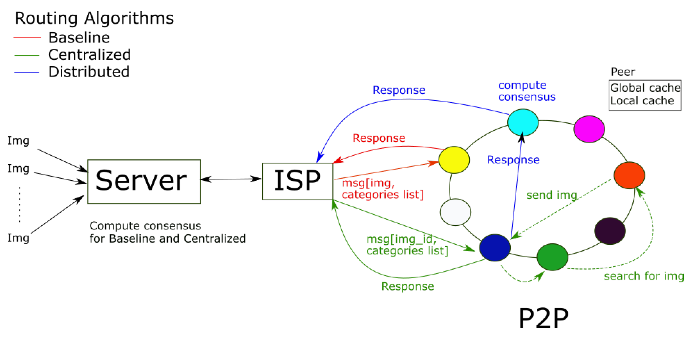
We chose the Centralized routing algorithm as the fixed value for the routing algorithm (ALG) parameter as it strikes a balance between the Baseline and the Distributed routing algorithms. This means it leverages the available computing and network resources in the P2P network while avoiding overloading the peers with the consensus calculation. Furthermore, the following experiments (Figure 8 and Figure 9) as well as prior research [13] comparing the performance of these three algorithms shows that the Centralized approach generally reports better results. We set $C=40\%$ to achieve a minimum consensus of 40%, and $H=50$. Increasing these values also increases the computational costs, while reducing them may lead to a decrease in the quality of volunteers’ votes. Finally, we set the $TTL=24$ h to avoid prematurely dropping tasks, while considering that a 24 h wait is sufficient for disaster scenarios [13,50].

Table 2. Impact of the controllable parameters (Routing algorithm, $C,H,TTL$) on the output metrics: consensus (Cons.), working time (workT), and the ISP utilization (USP_Util), for the index-based dynamic optimization approaches. For each output metric we also show the standard deviation (std). We highlight the best results in bold.

Params	Algorithm	Cons.	std	workT	std	ISP_Util	std
ALG	Index	0.414	0.202	228,000	6.481	0.399	0.112
ALG	IndexF	0.478	0.262	227,333	7.202	0.420	0.069
ALG	IndexLimit	0.395	0.217	230,667	8.571	0.346	0.060
ALG-C	Index	0.437	0.293	231,333	8.892	0.368	0.057
ALG-C	IndexF	0.387	0.163	227,500	4.764	0.414	0.114
ALG-C	IndexLimit	0.513	0.231	226,000	3.950	0.455	0.096
ALG-H	Index	0.997	0.001	102,167	14.470	0.465	0.211
ALG-H	IndexF	0.998	0.002	128,167	25.810	0.285	0.067
ALG-H	IndexLimit	0.992	0.007	111,833	17.429	0.403	0.254
ALG-H-C	Index	0.972	0.023	104,500	13.531	0.517	0.245
ALG-H-C	IndexF	0.993	0.012	122,333	31.602	0.414	0.228
ALG-H-C	IndexLimit	0.980	0.008	126,833	24.425	0.277	0.033
ALG-H-TLL	Index	0.998	0.001	102,333	14.264	0.465	0.208
ALG-H-TLL	IndexF	0.963	0.091	180,000	68.230	0.547	0.241
ALG-H-TLL	IndexLimit	0.994	0.007	99.167	8.353	0.623	0.334
ALG-TTL	Index	0.169	0.060	166,333	18.970	0.630	0.267
ALG-TTL	IndexF	0.210	0.087	179,500	19.087	0.658	0.314
ALG-TTL	IndexLimit	0.297	0.145	188,667	7.711	0.491	0.098
ALG-TTL-C	Index	0.187	0.144	170,333	19.336	0.690	0.300
ALG-TTL-C	IndexF	0.285	0.116	194,333	20.432	0.522	0.226
ALG-TTL-C	IndexLimit	0.319	0.143	195,667	27.259	0.560	0.223
All	Index	0.964	0.022	108,667	14.720	0.535	0.214
All	IndexF	0.960	0.060	134,000	29.604	0.349	0.056
All	IndexLimit	0.987	0.009	123,667	21.417	0.421	0.144
C	Index	0.490	0.307	228,667	33.146	0.578	0.313
C	IndexF	0.496	0.319	229,667	33.068	0.575	0.316
C	IndexLimit	0.515	0.317	228,833	32.443	0.575	0.316
H	Index	0.997	0.002	124,167	47.864	0.477	0.313
H	IndexF	0.998	0.001	118,667	42.908	0.471	0.294
H	IndexLimit	0.992	0.005	109,667	24.080	0.472	0.326
H-C	Index	0.980	0.019	136,833	46.893	0.462	0.301
H-C	IndexF	0.976	0.013	132,167	42.832	0.455	0.281
H-C	IndexLimit	0.987	0.023	113,833	25.143	0.429	0.267
H-TTL	Index	0.776	0.331	114,000	36.006	0.505	0.279
H-TTL	IndexF	0.900	0.148	113,833	36.191	0.492	0.279
H-TTL	IndexLimit	0.993	0.004	109,167	23.507	0.482	0.323
H-TTL-C	Index	0.774	0.286	121,000	25.675	0.502	0.259
H-TTL-C	IndexF	0.921	0.142	122,833	26.739	0.480	0.258
H-TTL-C	IndexLimit	0.991	0.013	114,000	20.986	0.438	0.269
TTL	Index	0.350	0.339	194,333	44.148	0.615	0.291
TTL	IndexF	0.384	0.329	199,500	24.882	0.582	0.309
TTL	IndexLimit	0.384	0.312	213,000	37.709	0.586	0.309
TTL-C	Index	0.236	0.105	189,500	50.919	0.616	0.292
TTL-C	IndexF	0.240	0.116	190,167	11.548	0.591	0.297
TTL-C	IndexLimit	0.379	0.323	197,833	27.709	0.602	0.297

shows the mean and standard deviation (std) reported by the Index, the IndexLimit, and the IndexF algorithms for the consensus (Cons.); the processing time of the platform (workT); and the ISP utilization (ISP_Util). We processed a total of $nQ$ = 10,000 images.

By controlling only the H parameter, the index-based algorithms achieve a consensus greater than 99%. If we only control the voting threshold C the algorithms achieve consensus values between 49% and 52%, the routing algorithm (ALG) allows us to obtain consensus between 39% and 48% when individually manipulated, and the $TTL$ allows us to achieve consensus values between 35% and 39%. Regarding the processing time (workT), by controlling the H parameter, the algorithms report values between 109 and 125 h, controlling the parameter C reports a workT between 228 and 230 h, the $TTL$ is between 194 and 213 h, and the routing algorithm ALG is between 228 and 231 h. Finally, controlling the H parameter individually allows us to achieve ISP average utilization values between 47% and 48%, the ALG is between 34% and 42%, the $TTL$ is between 58% and 62%, and the voting threshold C is between 57% and 58%.

When controlling different combinations of parameters, including all of them together (All), the highest percentage of consensus is 0,998, which is achieved by combining H and the routing algorithm ALG using the $IndexF$ approach. However, similar results are obtained with the other metric-indexed approaches and when using the H parameter or any combinations including H. Thus, the H parameter drastically impacts the percentage of consensus.

On the other hand, the lower processing time, 99.167,is reported by the $indexF$ approach with the ALG-H-$TTL$ combination of controllable parameters. In this case, the consensus reported is 0.994. However, the ISP utilization is higher than 60%. On the other hand, the Index approach with the same controllable parameter configuration manages to keep the average utilization of the ISP network close the limit of 40%, and the processing of the tasks is completed in approximately 102 h. Finally, when all parameters are controlled at the same time, the $Index$ approach returns a high consensus value of 0.964, a total processing time of 108 h, and the average ISP utilization is 53%. The $IndexF$ approach reports a consensus of 0.96, the processing time is 134 h, and the ISP utilization is 34%. The $IndexLimit$ achieves a consensus of 0.987, a processing time of 123 h, and the ISP utilization is 42%.

Therefore, in Table 2 we show that controlling some parameters in isolation, like the $TTL$ and C, does not help to achieve efficient results. On the other hand, the parameter H allows one—in most cases—to achieve a high level of consensus. When controlling H and ALG at the same time, we can reduce the average utilization of the ISP.

Figure 8 shows the average consensus obtained with different dynamic optimization approaches and when no optimization is applied (None). The x-axis shows the name of the routing algorithm used at the beginning of the experiment. At the top, we show the results obtained when $H=30$ at the beginning of the experiment, and at the bottom we show the results obtained when $H=50$. The results show that the Baseline routing algorithm obtains a 100% consensus for the case without optimization when the initial value of $H=30$, but with $H=50$ it reports a low consensus close to 30%. On the other hand, all dynamic parameter optimization approaches achieve consensus levels between 90% and 100%, with $DQL$-$Act$ being the one that obtains the lowest values.

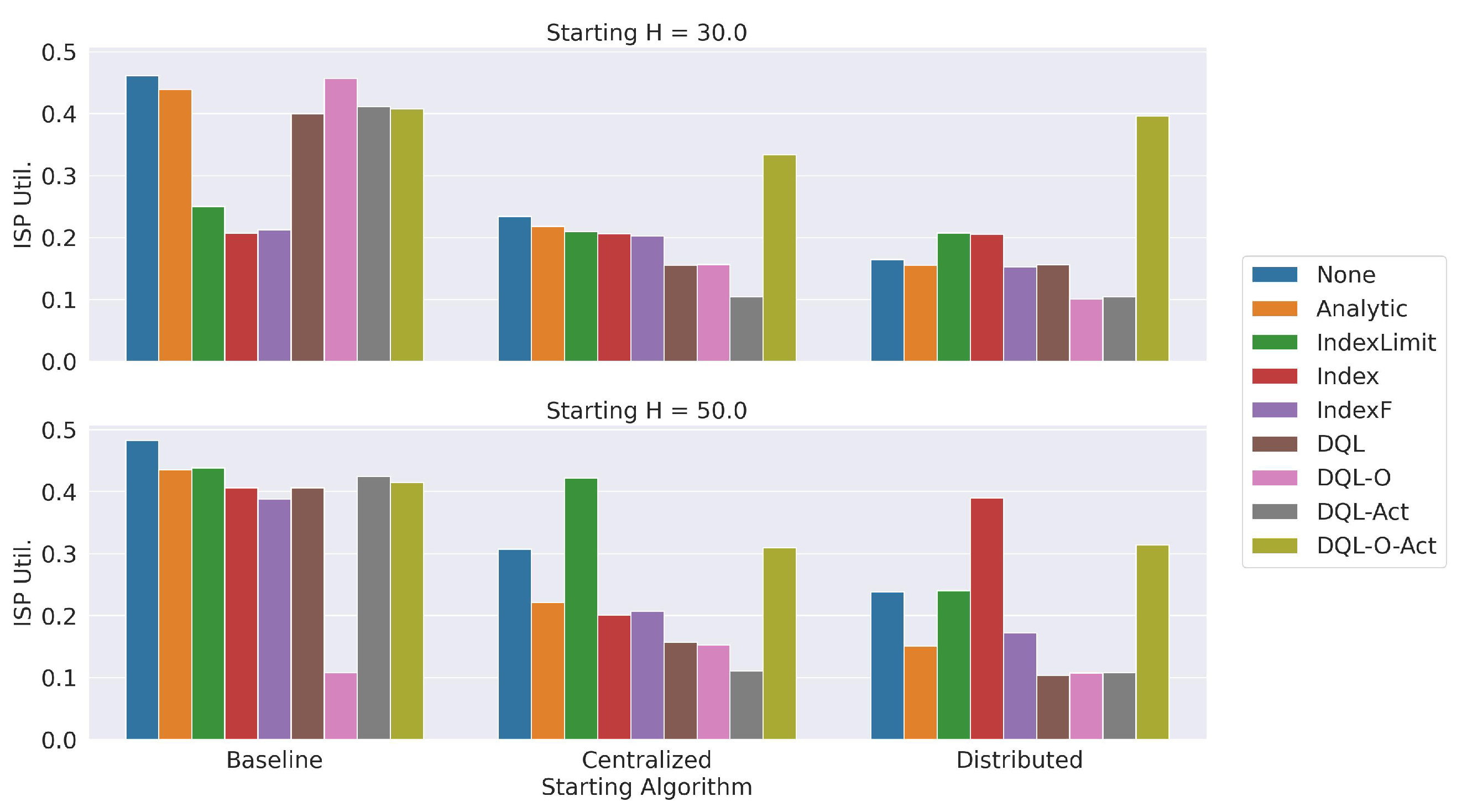
Figure 9 shows the average utilization of the ISP network. The x-axis shows the name of the routing algorithm used at the beginning of the experiment. Again, at the top we show the results obtained when $H=30$ at the beginning of the experiment, and at the bottom we show when $H=50$. The results show that the ISP utilization tends to be higher than 40% when the experiment begins with the Baseline routing algorithm, which uses point-to-point communication between the server and the peers through the ISP. If the initial value $H=30$, only the dynamic optimization approaches based on a metric index can keep the average utilization of the ISP below 40%. Meanwhile, when the initial value $H=50$, the DQL-O approach drastically reduces the ISP utilization. When we use the Centralized or Distributed routing algorithms at the beginning of the experiment and $H=30$, the results show that the $DQL$-o-$Act$ dynamic optimization approach reports the highest utilization. All the remaining approaches tend to keep the ISP utilization below 40%. With $H=50$, again the dynamic optimization approaches tend to keep the ISP utilization below 40%. Only the $IndexLimit$ approach, initializing the execution with the Centralized algorithm, and the $Index$ approach, using Distributed as the initial routing algorithm, report a high ISP utilization.

Figure 10 shows the time required to process the $nQ$ images. With an initial value $H=30$, we can reduce the processing time by 20% when applying a dynamic optimization approach. In this case, the $IndexLimit$ approach reports the lowest processing times. With $H=50$ and stating with the Baseline routing algorithm, we can reduce the processing time by 80% by using a dynamic optimization approach. In this case, the $DQL$ approach presents the lowest processing time when the experiment begins with the Baseline or with the Centralized routing algorithms. The index-based approaches present competitive results. Otherwise, when starting with the Distributed routing algorithm, the $Index$ approach presents the lowest processing time.

Overall, the analytical approach reports a good percentage of consensus and low processing times, but the ISP utilization tends to be high. Regarding the metric index-based approaches, all the proposed versions report a high percentage of consensus and an ISP utilization below 40%, but the $IndexLimite$ version reports lower processing times with $H=30$ and the $Index$ version with $H=50$. Finally, the $DQL$ approach is the one that generally obtains the best results for all the metrics among the reinforcement-learning-based approaches.

7.2. Execution Time of the Dynamic Optimization Approaches

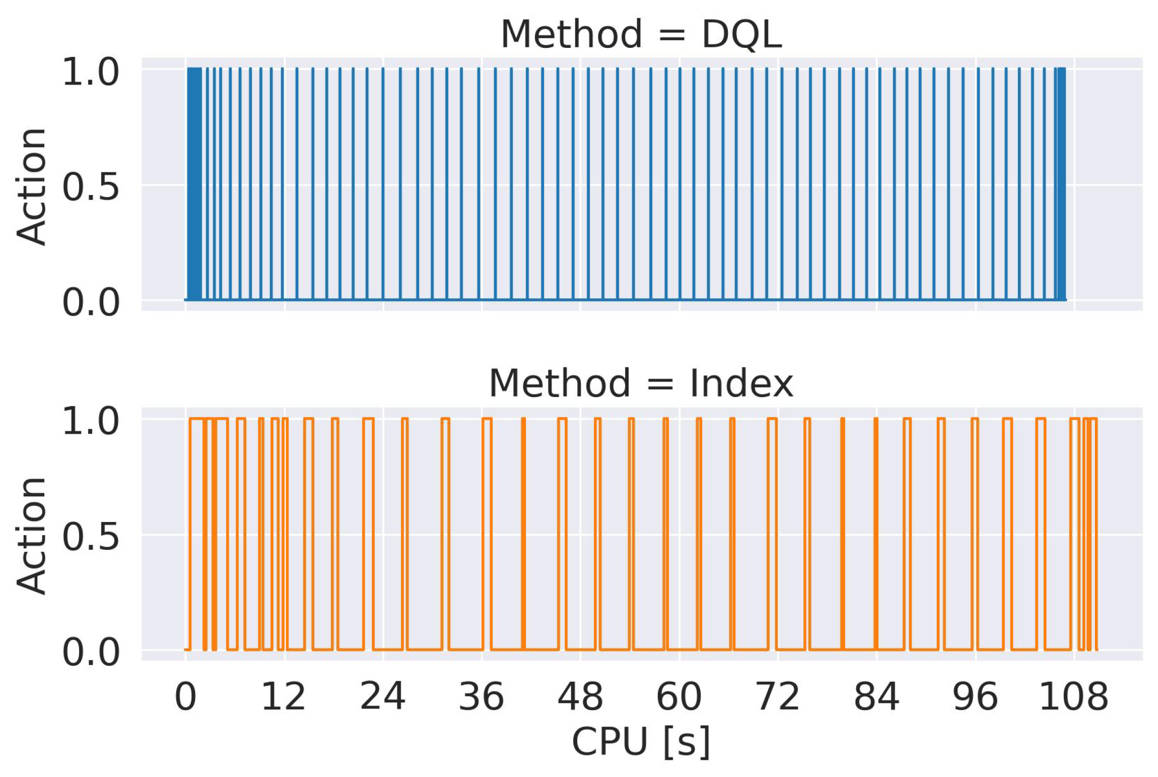
Figure 11 shows the CPU time of the actions performed by the parameter optimization approaches with the metric index ($Index$) and with DRL ($DQL$). The intervals in which the signal is 1 correspond to the intervals where the CPU is used by the $Index$ or the $DQL$, that is, the active intervals of the optimization algorithms. In periods when the signal is 0, only the crowdsoursing platform is active. The graph shows the results obtained for 10,000 images, an initial value of $H=50$, and applying the Distributed routing algorithm. Similar results were obtained for other configurations.

The results show that the $DQL$ reports a larger number of optimization actions, but each one is very fast. On the other hand, the $Index$ approach reports a lower number of optimization actions but each one consumes more time than in the case of the $DQL$. The result of accumulating the CPU time of the optimization actions of each algorithm is 23.86 s for the metric index-based approach and 11.73 ms for the optimization with $DQL$. However, the execution time of the simulation with both approaches tends to be similar, close to 108 s. Notice that the time of the crowdsourcing campaign is higher than 90 h; therefore, the execution times of both dynamic optimization approaches are negligible when operating on a real system.

Regarding the time required to set up the index-based dynamic optimization engine, it is important to notice that the database and the index are only built once, and it depends on the size of the database, but generally it takes a couple of hours at most. When using the $DQL$-based approach, we also have to build the configuration vectors (databases) from previous simulations and then we have to train the model. The training process can take several days, and it must be repeated for each trained model until the desired result is obtained. So, there is a higher uncertainty in the amount of time required to fine-tune the accuracy of the $DQL$-based approach.

7.3. Scalability

Figure 12 shows the percentage of consensus obtained with the dynamic optimization engine as we increase the value of $nQ$. The black bars represent the variation. The results show that with a larger number of images the approaches tend to present a lower consensus. This is more evident for the $DQL$-O, $DQL$-$Act$, and $DQL$-O-$Act$ approaches, while the percentage of consensus remains high—above 80%—for $IndexF$, $IndexLimit$, $Index$, and $DQL$.

Figure 13 shows the processing time ($workTime$) obtained for all the dynamic optimization approaches with different numbers of $nQ$. Again, results show that the $IndexLimit$, $Index$ and $DQL$ report the best results. The $IndexF$, presents a slightly lower performance. More importantly, the processing time reported by the dynamic optimization approaches for the case of 15,000 images is 42% lower than the approach without optimization (None).

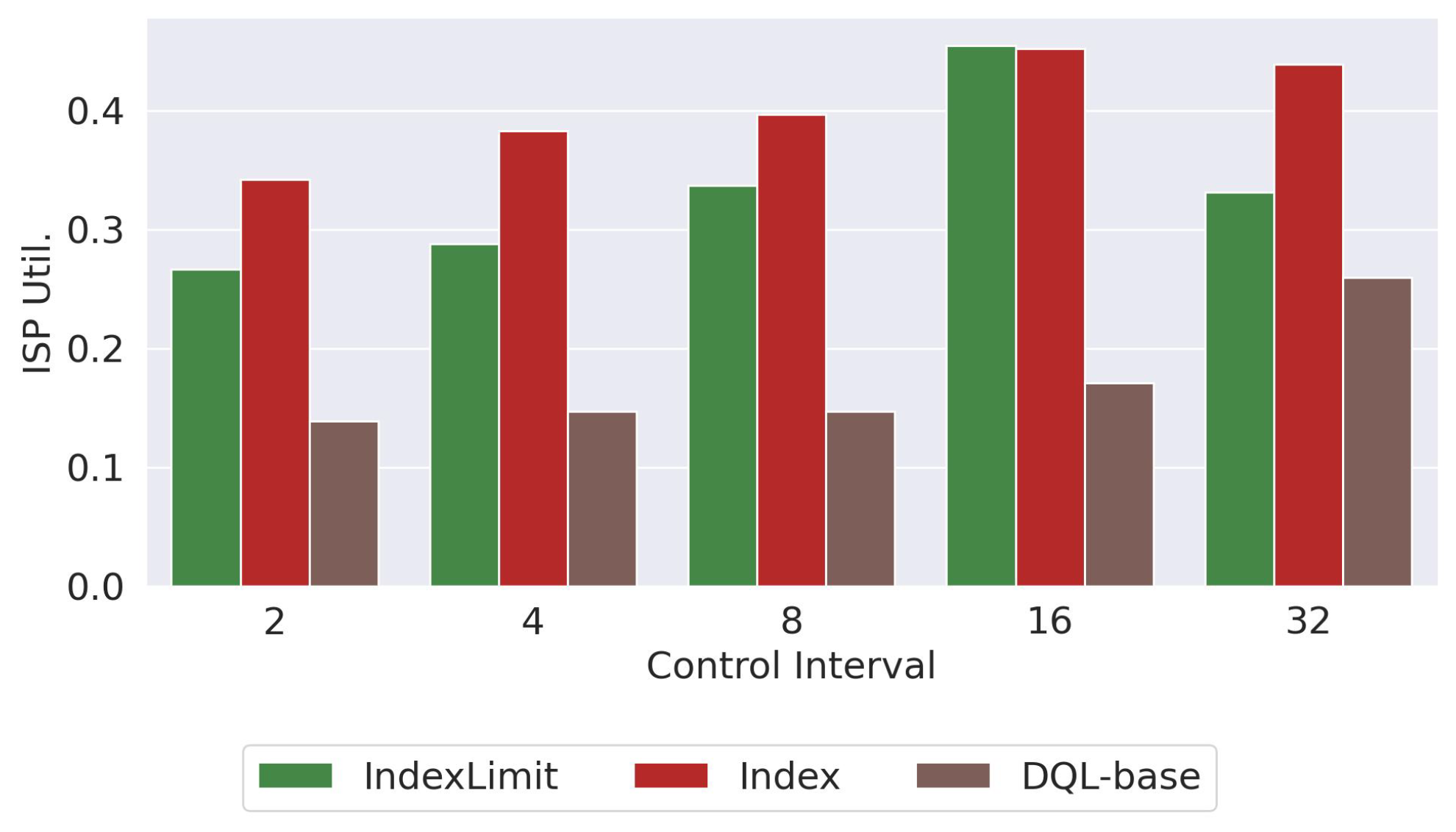
7.4. Size of the Control Window

This section discusses the impact of using different time intervals (called control intervals or control windows) to run the dynamic optimization engine. That is, as the crodwsourcing platform processes images, the dynamic optimization algorithm is activated every ${\Delta }_t$ units of time. We show the results obtained with $H=30$ and using the Baseline routing algorithm at the beginning of the experiment. In Figure 14, we show the ISP utilization obtained with an interval of ${\Delta }_t=\{2,4,8,16,32\}$ hours. 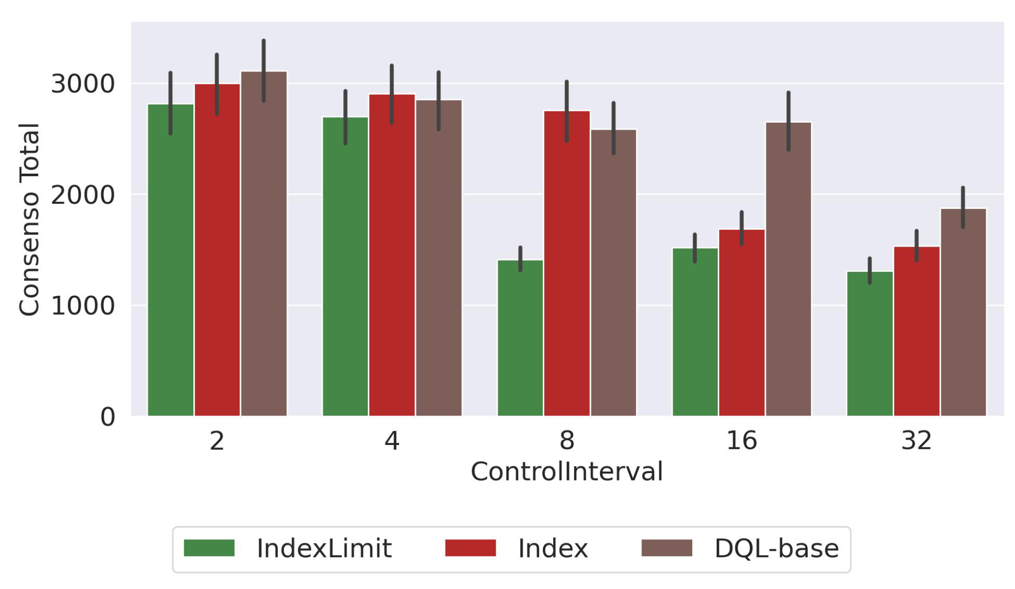Figure 15 shows the average consensus obtained and Figure 16 shows the processing time ($workTime$). We show the results for the $IndexLimit$, $Index$, and $DQL$ approaches, since similar trends have been observed for the other variants.

The results show that a larger ${\Delta }_t$ tends to increase the IPS utilization (Figure 14). This is mainly because as we increase the time in which the changes are made in the parameters, it takes more time to correctly adjust the values of the parameters. Then, as expected, a larger value of ${\Delta }_t$ increases the processing time (Figure 16) and decreases the consensus percentage not only because the parameter control takes more time to correctly adjust the values but also because a higher ISP utilization creates a bottleneck between the peers and the server and therefore the tasks take more time to be processed.

Therefore, a large value of ${\Delta }_t$ delays the parameter adjustment and can affect the performance of the platform. On the other hand, a small value of ${\Delta }_t$ changes the parameters of the platform more frequently, making the platform unstable (some tasks are solved with more peers than others, the routing algorithm can change every time interval, etc.). The results show that with a ${\Delta }_t=\{2,4,8\}$ all approaches achieve high consensus, low ISP utilization, and small processing times.

Additionally, using a small ${\Delta }_t$ time interval increases the CPU time of the metric index-based dynamic optimization approach by 66%. In the case of the $DQL$, the CPU time increases four times with the smallest ${\Delta }_t=2$. In other words, using small intervals allows one to obtain good estimates for the metrics evaluated at the cost of a longer simulation execution time. However, as shown in previous sections (in Figure 11), the execution time of the simulations is close to 100 s.

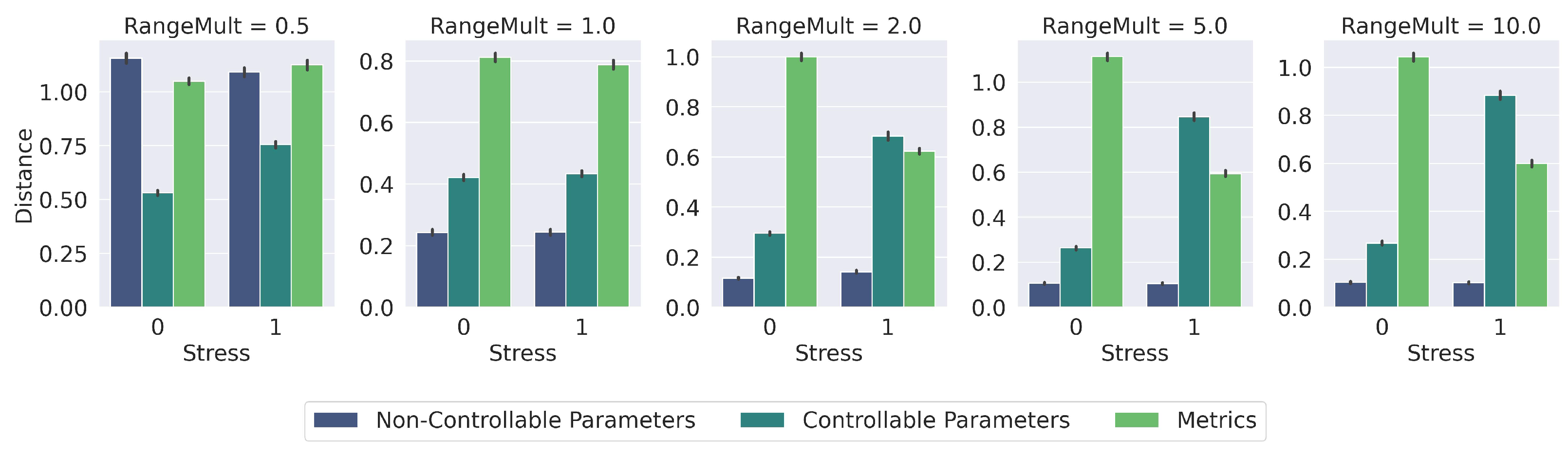
7.4.1. Constants $R_1,R_2$, and $R_3$

In this section, we evaluate the impact of the constants $R_1$, $R_2$, and $R_3$ that multiply the groups of variables in the vectors of the metric index. To this end, we use a ratio, $RangeMult$. If $RangeMult=10$, then, in stressful situations, $R_1=100$, $R_2=1$, and $R_3=10$. If the situation is not stressed, $R1=100$, $R_2=10$, and $R_3=1$. To assess the influence of $RangeMult$, we search for 1000 vectors in the index using different values of $RangeMult=\{0.5,1,2,5,10\}$, for situations with and without stress.

Figure 17 shows the distance between the subset of elements of the configuration vectors. That is, given a search vector $V_s$, the index searches the top-k closest configuration vector to $V_s$. Then, we report the distance between the subset formed of the non-controllable parameters of $V_s$ and the non-controllable parameters of the top-k vectors (blue bars). We also report the distance between the subset formed of the controllable parameters of $V_s$ and the controllable parameters of the top-k vectors (dark green bars). Finally, we report the distance between the subset formed of the metrics of $V_s$ and the metrics of the top-k vectors (light green bars). The x-axis indicates that the evaluated scenario is under stress, 1, or without stress, 0.

To retrieve configuration vectors that match the non-controllable parameters, it is expected to obtain the smallest distances between the values of this subset of elements of search vector $V_s$ and the top-k vectors. That is, we want to retrieve configurations with similar arrival rates and numbers of volunteers as in the current situation. In Figure 17, we show this is true when $RangeMult\ge 1$, since the blue bars report the lowest average distance.

In non-stress situations, it is expected that the distance reported by the subset of controllable parameters is less than the distances of the subset of metrics. On the other hand, under stress situations, it is expected that the distances of the subset of metrics is less than the distances reported by the subset of controllable parameters. This is fulfilled when $RangeMult\ge 2$. With larger values of $RangeMult$ this tendency is amplified. Therefore, to grant the appropriate priority to each subset of variables in stress and non-stress situations, we have to set $RangeMult\ge 1$.

7.4.2. Metric Index Evaluation

In this section, we analyze the impact of using different metric indices on the dynamic optimization engine. Figure 18 shows the average number of distance evaluations for a total of 1000 images. In this experiment, we use different metric space indices like the pivot index with 6 and 10 pivots and the Sparse Spatial Selection (SSS) [58] method with different values of the $\alpha$ parameter. We also evaluate the List of Clusters [59] index with different cluster sizes.

The results show that the performance of the List of Clusters (Lcluster) is highly dependent on the cluster size, reporting better results for larger cluster sizes. On the other hand, the results show that a six-pivot index—the configuration used in this work—obtains the best results. Nevertheless, if necessary, the metric index can be easily changed to a new one.

8. Conclusions

In this paper, we present and evaluate a metric space-based approach for the dynamic optimization of parameters. The proposed approach is devised to improve the performance of a crowdsourcing platform built with a P2P network designed to operate in the context of natural disasters and to deal with unexpected bursts of incoming requests. The context requires that the deployment of crowdsourcing campaigns achieves results in the shortest possible time and without saturating the platform’s resources.

The proposal incorporates the concept of similarity to give the platform more adequate parameter configurations according to the characteristics of the current workload and the size of the volunteer network. The proposal uses a metric database formed of vectors with elements describing the non-controllable parameters, controllable parameters, and metrics. We used a pivot index for the evaluation of the proposal, but other metric indices can be easily incorporated.

We presented two versions of the dynamic parameter optimization algorithm with metric indices and compared them with an analytical optimization approach and with different algorithms using deep reinforcement learning. We evaluated the processing time, the utilization of resources, and the voting consensus with different routing algorithms. The results show that the metric index dynamic optimization approach achieves competitive processing times, high voting consensus, and is capable of keeping the utilization below 40%. Additionally, we showed that the proposal can scale for a high number of tasks and that incorporating dynamic parameter optimization allows us to fulfill the platform’s performance requirements and also reduces the processing time by 40% when the platform is under a high workload.

As future work, we plan to incorporate other deep reinforcement learning algorithms to the platform. Furthermore, it would be interesting to incorporate more complex network topologies involving different communities of volunteers.

References

1. Jamal, A.; Al-Ahmadi, H.M.; Butt, F.M.; Iqbal, M.; Almoshaogeh, M.; Ali, S. Metaheuristics for Traffic Control and Optimization: Current Challenges and Prospects. In Search Algorithm—Essence of Optimization; Harkut, D.D.G., Ed.; IntechOpen: Rijeka, Croatia, 2021; Chapter 2. [Google Scholar] [CrossRef]
2. Li, F.; Su, Z.; Wang, G.M. An effective integrated control with intelligent optimization for wastewater treatment process. J. Ind. Inf. Integr. 2021, 24, 100237. [Google Scholar] [CrossRef]
3. Song, D.; Liu, J.; Yang, Y.; Yang, J.; Su, M.; Wang, Y.; Gui, N.; Yang, X.; Huang, L.; Hoon Joo, Y. Maximum wind energy extraction of large-scale wind turbines using nonlinear model predictive control via Yin-Yang grey wolf optimization algorithm. Energy 2021, 221, 119866. [Google Scholar] [CrossRef]
4. Yazdani, D.; Cheng, R.; Yazdani, D.; Branke, J.; Jin, Y.; Yao, X. A survey of evolutionary continuous dynamic optimization over two decades—Part A. IEEE Trans. Evol. Comput. 2021, 25, 609–629. [Google Scholar] [CrossRef]
5. Yazdani, D.; Cheng, R.; Yazdani, D.; Branke, J.; Jin, Y.; Yao, X. A survey of evolutionary continuous dynamic optimization over two decades—Part B. IEEE Trans. Evol. Comput. 2021, 25, 630–650. [Google Scholar] [CrossRef]
6. Wang, P.; Qin, J.; Li, J.; Wu, M.; Zhou, S.; Feng, L. Dynamic Optimization Method of Wireless Network Routing Based on Deep Learning Strategy. Mob. Inf. Syst. 2022, 2022. [Google Scholar] [CrossRef]
7. Tuli, S.; Poojara, S.R.; Srirama, S.N.; Casale, G.; Jennings, N.R. COSCO: Container Orchestration Using Co-Simulation and Gradient Based Optimization for Fog Computing Environments. IEEE Trans. Parallel Distrib. Syst. 2022, 33, 101–116. [Google Scholar] [CrossRef]
8. Karthick, T.; Charles Raja, S.; Jeslin Drusila Nesamalar, J.; Chandrasekaran, K. Design of IoT based smart compact energy meter for monitoring and controlling the usage of energy and power quality issues with demand side management for a commercial building. Sustain. Energy Grids Netw. 2021, 26, 100454. [Google Scholar]
9. Marín, M.; Gil-Costa, V.; Inostrosa-Psijas, A.; Bonacic, C. Hybrid capacity planning methodology for web search engines. Simul. Model. Pract. Theory 2019, 93, 148–163. [Google Scholar] [CrossRef]
10. Gosavi, A. Simulation-Based Optimization; Springer: Berlin/Heidelberg, Germany, 2015. [Google Scholar]
11. Shi, Y.; Sagduyu, Y.E.; Erpek, T. Reinforcement learning for dynamic resource optimization in 5G radio access network slicing. In Proceedings of the 2020 IEEE 25th International Workshop on Computer Aided Modeling and Design of Communication Links and Networks (CAMAD), Pisa, Italy, 14–16 September 2020; IEEE: Piscataway, NJ, USA, 2020; pp. 1–6. [Google Scholar]
12. Mosavi, A.; Faghan, Y.; Ghamisi, P.; Duan, P.; Ardabili, S.F.; Salwana, E.; Band, S.S. Comprehensive review of deep reinforcement learning methods and applications in economics. Mathematics 2020, 8, 1640. [Google Scholar] [CrossRef]
13. Loor, F.; Manriquez, M.; Gil-Costa, V.; Marín, M. Feasibility of P2P-STB based crowdsourcing to speed-up photo classification for natural disasters. Clust. Comput. 2022, 25, 279–302. [Google Scholar] [CrossRef]
14. Chávez, E.; Navarro, G.; Baeza-Yates, R.; Marroquín, J.L. Searching in metric spaces. ACM Comput. Surv. 2001, 33, 273–321. [Google Scholar] [CrossRef]
15. Bebis, G. Fingerprint Indexing. In Encyclopedia of Biometrics; Li, S.Z., Jain, A., Eds.; Springer: Boston, MA, USA, 2009; pp. 491–496. [Google Scholar] [CrossRef]
16. Gil-Costa, V.; Santos, R.L.; Macdonald, C.; Ounis, I. Modelling efficient novelty-based search result diversification in metric spaces. J. Discret. Algorithms 2013, 18, 75–88. [Google Scholar] [CrossRef]
17. Echihabi, K.; Zoumpatianos, K.; Palpanas, T. High-dimensional similarity search for scalable data science. In Proceedings of the 2021 IEEE 37th International Conference on Data Engineering (ICDE), Chania, Greece, 19–22 April 2021; IEEE: Piscataway, NJ, USA, 2021; pp. 2369–2372. [Google Scholar]
18. Zezula, P.; Amato, G.; Dohnal, V.; Batko, M. Similarity Search: The Metric Space Approach; Advances in Database Systems; Springer: New York, NY, USA, 2006; Volume 32. [Google Scholar]
19. Samet, H. Foundations of Multidimensional and Metric Data Structures (The Morgan Kaufmann Series in Computer Graphics and Geometric Modeling); Morgan Kaufmann Publishers Inc.: Burlington, MA, USA, 2005. [Google Scholar]
20. Mamede, M.; Barbosa, F. Range queries in natural language dictionaries with recursive lists of clusters. In Proceedings of the 22nd International Symposium on Computer and Information Sciences, ISCIS, Ankara, Turkey, 7–9 November 2007. [Google Scholar]
21. Baeza-Yates, R.; Cunto, W.; Manber, U.; Wu, S. Proximity Matching Using Fixed-Queries Trees. In Proceedings of the 5th Annual Symposium on Combinatorial Pattern Matching, CPM, LNCS 807, Asilomar, CA, USA, 5–8 June 1994; pp. 198–212. [Google Scholar]
22. Mico, L.; Oncina, J.; Vidal, E. A new version of the nearest-neighbor approximating and eliminating search (AESA) with linear preprocessing-time and memory requirements. Pattern Recogn. Lett. 1994, 15, 9–17. [Google Scholar] [CrossRef]
23. Gennaro, C.; Mordacchini, M.; Orlando, S.; Rabitti, F. A Scalable Distributed Data Structure for Multi-Feature Similarity Search. In Proceedings of the Sixteenth Italian Symposium on Advanced Database Systems, SEBD, Mondello, PA, Italy, 22–25 June 2008; pp. 302–309. [Google Scholar]
24. Chen, L.; Gao, Y.; Zheng, B.; Jensen, C.S.; Yang, H.; Yang, K. Pivot-based metric indexing. In Proceedings of the VLDB Endowment: 43rd International Conference, Munich, Germany, 28 August–1 September 2017. [Google Scholar]
25. Gil-Costa, V.; Marin, M.; Reyes, N. Parallel query processing on distributed clustering indexes. J. Discret. Algorithms 2009, 7, 3–17. [Google Scholar] [CrossRef]
26. Argentina, S.; Quinteros, A.; García, R.H.; Frati, F.E.; Barrientos, R.J. A Comparative Analysis of Massive Finger-Vein Recognition Algorithms: From Energy Consumption Perspective. In Proceedings of the 2022 41st International Conference of the Chilean Computer Science Society (SCCC), Santiago, Chile, 21–25 November 2022; pp. 1–6. [Google Scholar]
27. Artigas-Fuentes, F.J.; Badía, J.M. Accessing very high dimensional spaces in parallel. J. Supercomput. 2017, 73, 176–189. [Google Scholar] [CrossRef]
28. Safaee, S.; Mirabi, M.; Safaei, A.A. StreamFilter: A framework for distributed processing of range queries over streaming data with fine-grained access control. Clust. Comput. 2024, 73, 1573–7543. [Google Scholar] [CrossRef]
29. Novak, D.; Batko, M.; Zezula, P. Large-scale similarity data management with distributed Metric Index. Inf. Process. Manag. 2012, 48, 855–872. [Google Scholar] [CrossRef]
30. Catalyurek, U.V.; Boman, E.G.; Devine, K.D.; Bozdağ, D.; Heaphy, R.T.; Riesen, L.A. A repartitioning hypergraph model for dynamic load balancing. Parallel Distrib. Comput. 2009, 69, 711–724. [Google Scholar] [CrossRef]
31. Yang, K.; Ding, X.; Zhang, Y.; Chen, L.; Zheng, B.; Gao, Y. Distributed similarity queries in metric spaces. Data Sci. Eng. 2019, 4, 93–108. [Google Scholar] [CrossRef]
32. Gadaleta, M.; Chiariotti, F.; Rossi, M.; Zanella, A. D-DASH: A deep Q-learning framework for DASH video streaming. IEEE Trans. Cogn. Commun. Netw. 2017, 3, 703–718. [Google Scholar] [CrossRef]
33. Ding, D.; Fan, X.; Zhao, Y.; Kang, K.; Yin, Q.; Zeng, J. Q-learning based dynamic task scheduling for energy-efficient cloud computing. Future Gener. Comput. Syst. 2020, 108, 361–371. [Google Scholar] [CrossRef]
34. Luong, N.C.; Hoang, D.T.; Gong, S.; Niyato, D.; Wang, P.; Liang, Y.C.; Kim, D.I. Applications of deep reinforcement learning in communications and networking: A survey. IEEE Commun. Surv. Tutor. 2019, 21, 3133–3174. [Google Scholar] [CrossRef]
35. Wang, L.; Pan, Z.; Wang, J. A review of reinforcement learning based intelligent optimization for manufacturing scheduling. Complex Syst. Model. Simul. 2021, 1, 257–270. [Google Scholar] [CrossRef]
36. Yang, H.; Li, W.; Wang, B. Joint optimization of preventive maintenance and production scheduling for multi-state production systems based on reinforcement learning. Reliab. Eng. Syst. Saf. 2021, 214, 107713. [Google Scholar] [CrossRef]
37. Rabault, J.; Ren, F.; Zhang, W.; Tang, H.; Xu, H. Deep reinforcement learning in fluid mechanics: A promising method for both active flow control and shape optimization. J. Hydrodyn. 2020, 32, 234–246. [Google Scholar] [CrossRef]
38. Yu, C.; Liu, J.; Nemati, S.; Yin, G. Reinforcement learning in healthcare: A survey. ACM Comput. Surv. (CSUR) 2021, 55, 1–36. [Google Scholar] [CrossRef]
39. Kompella, V.; Capobianco, R.; Jong, S.; Browne, J.; Fox, S.; Meyers, L.; Wurman, P.; Stone, P. Reinforcement learning for optimization of COVID-19 mitigation policies. arXiv 2020, arXiv:2010.10560. [Google Scholar]
40. Boulesnane, A.; Meshoul, S. Reinforcement learning for dynamic optimization problems. In Proceedings of the Genetic and Evolutionary Computation Conference Companion, Lille, France, 10–14 July 2021; pp. 201–202. [Google Scholar]
41. Forootani, A.; Zarch, M.G.; Tipaldi, M.; Iervolino, R. A stochastic dynamic programming approach for the machine replacement problem. Eng. Appl. Artif. Intell. 2023, 118, 105638. [Google Scholar] [CrossRef]
42. Rowstron, A.; Druschel, P. Pastry: Scalable, Decentralized Object Location, and Routing for Large-Scale Peer-to-Peer Systems. In Proceedings of the Middleware 2011, Lisbon, Portugal, 12–16 December 2011; Guerraoui, R., Ed.; Springer: Berlin/Heidelberg, Germany, 2001; pp. 329–350. [Google Scholar]
43. Corradi, A.; Fanelli, M.; Foschini, L. VM consolidation: A real case based on OpenStack Cloud. Future Gener. Comput. Syst. 2014, 32, 118–127. [Google Scholar] [CrossRef]
44. Marzolla, M. Libcppsim: A Simula-like, portable process-oriented simulation library in C++. In Proceedings of the 18th European Simulation Multiconference, ESM’04, Magdeburg, Germany, 13–16 June 2004; pp. 222–227. [Google Scholar]
45. Xia, G.S.; Bai, X.; Ding, J.; Zhu, Z.; Belongie, S.; Luo, J.; Datcu, M.; Pelillo, M.; Zhang, L. DOTA: A Large-Scale Dataset for Object Detection in Aerial Images. In Proceedings of the IEEE Conference on Computer Vision and Pattern Recognition (CVPR), Salt Lake City, UT, USA, 18–23 June 2018. [Google Scholar]
46. Cheng, G.; Han, J. A survey on object detection in optical remote sensing images. ISPRS J. Photogramm. Remote Sens. 2016, 117, 11–28. [Google Scholar] [CrossRef]
47. Alam, F.; Ofli, F.; Imran, M. Crisismmd: Multimodal twitter datasets from natural disasters. In Proceedings of the Twelfth International AAAI Conference on Web and Social Media, Palo Alto, CA, USA, 25–28 June 2018. [Google Scholar]
48. Bhavaraju, S.K.T.; Beyney, C.; Nicholson, C. Quantitative analysis of social media sensitivity to natural disasters. Int. J. Disaster Risk Reduct. 2019, 39, 101251. [Google Scholar] [CrossRef]
49. Imran, M.; Mitra, P.; Castillo, C. Twitter as a lifeline: Human-annotated twitter corpora for NLP of crisis-related messages. arXiv 2016, arXiv:1605.05894. [Google Scholar]
50. Kurkcu, A.; Zuo, F.; Gao, J.; Morgul, E.F.; Ozbay, K. Crowdsourcing incident information for disaster response using twitter. In Proceedings of the Transportation Research Board 96th Annual Meeting, Washington, DC, USA, 8–12 January 2017; pp. 1–17. [Google Scholar]
51. Murthy, D.; Gross, A.J. Social media processes in disasters: Implications of emergent technology use. Soc. Sci. Res. 2017, 63, 356–370. [Google Scholar] [CrossRef] [PubMed]
52. Danylo, O.; Moorthy, I.; Sturn, T.; See, L.; Laso Bayas, J.C.; Domian, D.; Fraisl, D.; Giovando, C.; Girardot, B.; Kapur, R.; et al. The Picture Pile tool for rapid image assessment: A demonstration using Hurricane Matthew. ISPRS Ann. Photogramm. Remote Sens. Spat. Inf. Sci. 2018, 4, 27–32. [Google Scholar] [CrossRef]
53. Rogstadius, J.; Vukovic, M.; Teixeira, C.A.; Kostakos, V.; Karapanos, E.; Laredo, J.A. CrisisTracker: Crowdsourced social media curation for disaster awareness. IBM J. Res. Dev. 2013, 57, 4:1–4:13. [Google Scholar] [CrossRef]
54. Salk, C.F.; Sturn, T.; See, L.; Fritz, S. Limitations of majority agreement in crowdsourced image interpretation. Trans. GIS 2017, 21, 207–223. [Google Scholar] [CrossRef]
55. Falcão, I.W.; Seruffo, M.C.; Souza, D.D.S.; Cardoso, D.L.; Ferreira, J.J.; Da Silva, M.S. A Comparative Analysis of Local and Cloud Access Assessment for Multimodal Interactive Application. In Proceedings of the 2018 4th International Conference on Cloud Computing Technologies and Applications, Cloudtech Brussels, Belgium, 26–28 November 2018. [Google Scholar]
56. Qarout, R.K.; Checco, A.; Bontcheva, K. Investigating stability and reliability of crowdsourcing output. In Proceedings of the CEUR Workshop Proceedings, Zürich, Switzerland, 14 December 2018; Volume 2276, pp. 83–87. [Google Scholar]
57. Mnih, V.; Kavukcuoglu, K.; Silver, D.; Rusu, A.A.; Veness, J.; Bellemare, M.G.; Graves, A.; Riedmiller, M.; Fidjeland, A.K.; Ostrovski, G.; et al. Human-level control through deep reinforcement learning. Nature 2015, 518, 529–533. [Google Scholar] [CrossRef]
58. Pedreira, O.; Brisaboa, N.R. Spatial selection of sparse pivots for similarity search in metric spaces. In Proceedings of the International Conference on Current Trends in Theory and Practice of Computer Science, Harrachov, Czech Republic, 20–26 January 2007; Springer: Berlin/Heidelberg, Germany, 2007; pp. 434–445. [Google Scholar]
59. Chávez, E.; Navarro, G. A compact space decomposition for effective metric indexing. Pattern Recognit. Lett. 2005, 26, 1363–1376. [Google Scholar] [CrossRef]
Figure 1. Pre-calculated distances between the pivots ( P 1 P N ) and every object ( o 1 o M ) in the metric space database.
Futureinternet 16 00202 g001
Figure 2. General scheme of the P2P-based crowdsourcing platform for image processing. Each peer is responsible for processing objects of different colors.
Futureinternet 16 00202 g002
Figure 4. Groups of variables inside the vectors that compose the metric database.
Futureinternet 16 00202 g004
Figure 5. Steps involved in the building phase of the dynamic optimization engine.
Futureinternet 16 00202 g005
Figure 6. ISP utilization: At time T 1 , the network utilization exceeds 40%, indicating a state of stress. However, by time T 2 , the network utilization decreases, and the platform returns to normal operation.
Futureinternet 16 00202 g006
Figure 7. Distribution of the arrival of images used in the experiments.
Futureinternet 16 00202 g007
Figure 8. Percentage of consensus reported with different dynamic optimization approaches and with no optimization (None).
Futureinternet 16 00202 g008
Figure 9. Average ISP network utilization obtained with different dynamic optimization approaches and with no optimization (None).
Futureinternet 16 00202 g009
Figure 10. Processing time (workTime) obtained with the different dynamic optimization approaches and with no optimization (None).
Futureinternet 16 00202 g010
Figure 11. Execution time reported by the I n d e x and D Q L optimization approaches when processing 10,000 images. We set the Distributed algorithm as the initial routing algorithm with an initial parameter H = 50 .
Futureinternet 16 00202 g011
Figure 12. Percentage of consensus obtained with the dynamic optimization approaches. We set H = 50 and the platform received 5000, 10,000, and 15,000 images.
Futureinternet 16 00202 g012
Figure 13. Processing time reported by the dynamic optimization approaches. We set the initial value of H = 50 and the platform receives 5000, 10,000 and 15,000 images.
Futureinternet 16 00202 g013
Figure 14. Average ISP utilization obtained with different values of the control interval.
Futureinternet 16 00202 g014
Figure 15. Consensus percentage obtained with different control interval values.
Futureinternet 16 00202 g015
Figure 16. Processing time obtained with different control interval values.
Futureinternet 16 00202 g016
Figure 17. Number of distance evaluations for different values for the constants R 1 , R 2 , and R 3 in the metric indices.
Futureinternet 16 00202 g017
Figure 18. Number of computations (distance evaluations) achieved with different metric space indices.
Futureinternet 16 00202 g018