4.1. Basic MA
The MA combines all effect size estimates of a common variable of interest reported by the collected articles, assigning more weight to more precise econometric results. Hence, the initial step of the MA is developed around the idea of meta-averages.
Therefore, the first question is: once all the collected estimates are combined, what is the true underlying growth effect of land inequality? The initial answer is a set of basic calculations that compute weighted means, which might differ substantially from the mean. Two weighted averages can be computed using the pooled fixed effect estimator (FEE) and the pooled random effect estimator (REE). The former assumes that there is no heterogeneity among studies’ results and the different magnitude of the estimates is due to sampling variation; the latter assumes heterogeneity among studies results.
Statistically, the underlying hypothesis in the FEE is that all effect sizes are equal, for example
, where
represents the effect of size of the
jth observation (in our case,
j = 1, 2, 3, …, 180) and
β is the true effect size, or population effect size [
64]. The observed effects will be distributed around α (the common effect), and will have a variance σ
2 that depends primarily on the sample size for each study. Hence, the weighted average effect is calculated with weights that are inversely proportional to the variance, and as a result, point estimates have greater weights associated to smaller standard errors [
65].
The REE assumes that all analyses are estimating different (random) treatment effects [
66]. The combined effect
β, therefore, represents an average of the population of true effects, and the variance associated with each effect size has two components: one regarding the sample level, as in the fixed effect model (within-variance), and the other one regarding the random effect variance (between-variance). Hence, the weights are inversely proportional to an estimate of between-study heterogeneity,
, and are equal to (
). A weighted least squares (WLS) estimate can be obtained regressing the
t-statistic of the estimated coefficients (
) on the inverse of their standard errors; it gives more efficient estimates and corrects for heteroscedasticity.
Table 1 reports the results of the basic MA. Considering the fact that the distribution of the PCC is truncated (the coefficient ranges from −1 to 1), and that it might cause an asymmetry, we also computed the Fisher’s z-transformed correlation [
67]:
For a robustness check, both MA results for both PCC and Fisher’s z-transformed correlation are reported in the table.
Table 1 displays pooled estimates of the effect size of land inequality, computed as simple means, weighted averages, FE, and RE estimates. All averages were statistically significant at 1% level. The simple average was equal to −0.19 in the case of the PCC and −0.20 in the case of the Fisher’s z-transformed correlation. However, with a highly skewed distribution, the weighted average was a more appropriate summarizing measure. The FEE and WLS estimates led to the same averages, but the confidence interval was slightly wider for the WLS estimate. The fixed effect of the PCC showed a value of −0.13, as opposed to the random effect, which showed a value of −0.17.
Results were slightly higher if Fisher’s z-transformed correlation was used; either way, the two distributions presented the same behavior. Hence, the PCCs were used in the ensuing analysis.
In summary, the preliminary result of our MA is that land inequality seemed to influence growth negatively: there was a trade–off between land inequality and economic growth. These findings may, however, be greatly affected by the presence of publication bias, e.g., when editors or referees, but also researchers, have a preference for results that are statistically significant and with a direction in line with the theoretical predictions.
4.2. Publication Selection Bias
Journal editors and authors may be inclined to report econometric results in a certain direction or there may be a tendency to publish only statistically significant findings, leaving aside non-significant findings or studies. This behavior produces the so-called “publication bias” [
66]. As already widely established by the literature, any simple overall MA should be interpreted with caution due to the possible presence of heterogeneity and/or publication bias in empirical findings [
68].
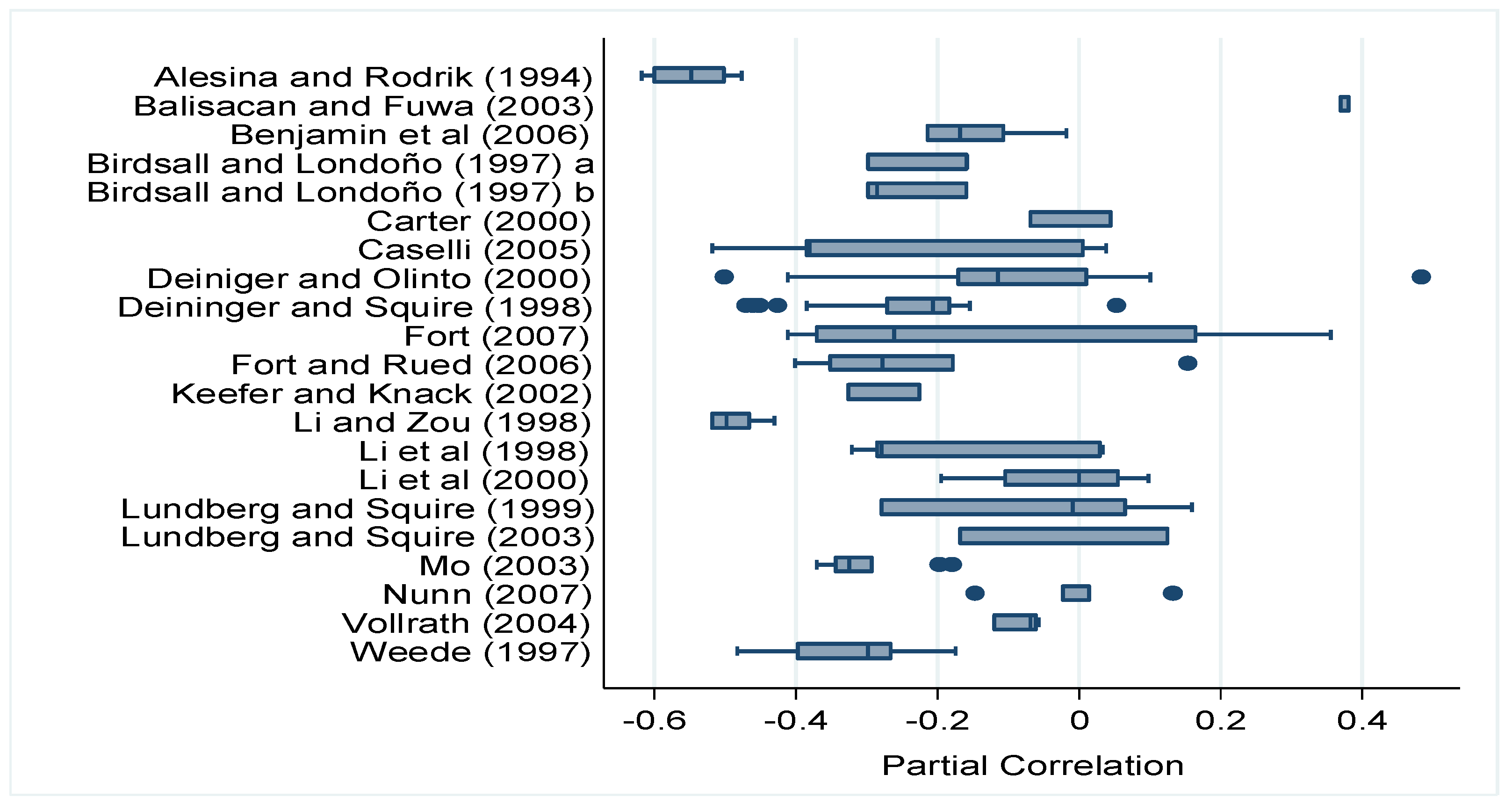
Figure 1 shows the heterogeneity of the results across studies: the results range from negative to positive values and are less or more economically significant. Even if the expectation of a negative growth effect of land inequality is by and large confirmed, 12 studies found evidence of positive effects.
The so-called Q-test is a formal way to test the hypothesis of heterogeneity (
) versus the alternative that at least one estimate differs. If
H0 is true, the Q-test has an asymptotic chi-squared distribution with
k − 1 degrees of freedom [
64]. In our meta sample, the hypothesis of heterogeneity is accepted and the null hypothesis of homogeneity is rejected with a
p-value < 0.001 (Q-test is 1350.88 with 179 degrees of freedom). Higgins and Thompson [
65] suggest the I
2 index to measure the share of variation of point estimates as a result of heterogeneity rather than sampling error. In our meta sample I
2 is equal to 86.75%, which reveals a high degree of heterogeneity. Therefore, considering these results, we are going to explain such heterogeneity in the effect sizes in the last section using a meta-regression analysis.
A popular plot to investigate the publication bias is the funnel plot [
69] that compares the estimated coefficient of the impact of land inequality on growth from each study and the inverse of its standard error, as a measure of precision. Publication bias may lead to asymmetrical funnel plots.
The funnel graph in
Figure 2 seems to be asymmetrical with a tendency to values on the left side (negative values). The solid vertical line illustrates the meta-average, suggesting a small negative effect of land inequality on economic growth.
However, visual inspections are subjective and somehow ambiguous [
70], and the funnel asymmetry test (FAT-PET) allows one to identify the asymmetry of the funnel plot by means of a regression between the collected effect sizes and respective standard errors; namely, the test determines if the intercept deviates significantly from zero [
69]. The WLS version, preferred to the OLS since meta-regression errors are likely to be heteroscedastic [
63], is as follows:
In the absence of publication selection, the overall effect size will vary randomly around the “true” value, , independently of its standard error; this means that the null hypothesis should be accepted. Another advantage of the use of the WLS model is that, according to Equation (5), the dependent variable in our model is no longer censored.
To account for the fact that estimates within one study are not statistically independent, we adopt a “robust with cluster” procedure to adjust standard errors for intra-study correlation. This is a common solution in meta-analysis literature [
71,
72], which relaxes the independent and identically distributed (i.i.d.) assumption of independent errors, and corrects for potential unobserved correlation among errors within clusters of observations.
In
Table 2, we explore the publication bias by implementing the FAT-PET using WLS, panel, and multilevel models.
Table 2 shows that the estimated coefficient
was significantly different from zero only in the case of the WLS model (column 1), signaling the presence of publication bias, while in the other three models (columns 2–4), it was not significantly different from zero, which does not confirm the existence of publication bias. Moreover, the estimated coefficient
was always negative, even if it was significant only when fixed-effect panel model was used (column 2), providing evidence of a genuinely negative effect.
Stanley and Doucouliagos [
73] argue that in the presence of a genuine effect, the FAT-PET is downwardly bias, and suggest the “precision-effect estimate with standard error” (PEESE) model to correct potential publication bias:
The PEESE results shown in
Table 3 suggest that, after correcting for publication bias, there existed a significant and negative effect of land inequality on economic growth.
In the following, we implement a multiple meta-regression analysis (MRA) to explain the diversity in findings in the literature controlling for various characteristics of the collected studies.
4.3. Multiple Meta-Regression Analysis
In our MRA, we include as moderator a set of control variables reflecting features of the studies considered and try to explain the heterogeneity in the MA sample.
We select seven characteristics: (i) the development level of the countries included in the sample, (ii) the theoretical framework, (iii) the definitions of the dependent variable, (iv) the estimation techniques, (v) the structure of the data, (vi) the database used for growth and for land inequality, and (vii) published versus unpublished articles. Finally, we added dummies for periods in order to collect studies using data related only to specific time periods.
Results for the overall sample are shown in
Table 4. In columns 1 and 2, we took into account the potential publication bias and estimated the multiple WLS-MRA and the PEESE correction, and in column 3 we simply dropped the standard error from the regression in order to check how the results change.
Adding our set of moderators, we could capture quite a lot of the heterogeneity in the partial correlation coefficients. Since the FAT coefficient was statistically insignificant (in column 1), it did not appear as evidence of publication selection. The overall inequality effect on economic growth was negative and statistically significant, ( = −0.44 with p-value < 0.05). After correcting for potential publication selection bias and by looking at results in column 2, we still found a significant and negative effect, ( = −0.41 with p-value < 0.01). Such a result was also confirmed by the simple MRA (column 3); however, without filtering out publication bias, the estimated effect was lower ( = −0.33 with p-value < 0.01).
From a methodological point of view, the estimated coefficients of dummies for country groups included in our multiple MRA indicate how results from analyses focusing on specific countries differ. In particular, we investigated how the effect size differed among studies that included in their analysis countries with different levels of development. We added dummies Developed, with value equal to one when the primary study includes only developed countries, and Developing, with value equal to one when the primary study includes only developing countries. The dummy sample of countries remained as the control variable, corresponding to studies that included both developed and developing countries. Statistically significant coefficients of these country dummies supported the idea that inequality affects the developed countries less and the developing countries more. Part of the heterogeneity can be explained by which sample of countries was considered.
Concerning the dummies describing the theoretical framework, we included dummies for “Endogenous Human Capital (HC)” and “Political Economy Models.” The omitted category was a dummy related to the set of the empirically oriented literature on distribution. The dummy for historical approaches was dropped due to collinearity, since it included only one study. The idea was that studies based on the same theoretical framework tended to include the same set of control variables. We found that all controls had negative and statistically significant coefficients, hence the theoretically grounded analyses tended to confirm the negative results predicted by theory: empirical tests tended to produce lower effects.
The MRA included controls for the dependent variable used as a measure of economic growth, as well as for the structure of the data and the estimators adopted. We distinguished studies that compute the economic growth rate using data on GDP from those that used data on income. Even if conceptually, the terms income and GDP were equal in national economic accounting, in practice their data may differ due to the use of different sources of information. Results in
Table 4 show that only the coefficient of the dummy GDP was equal to 1 when the dependent variable used was the growth rate of GDP and was statistically significant and negative, hence land inequality seemed to affect GDP more than income growth. The estimated coefficient for the dummy “Agricultural production” was not statistically significant, and sectoral analysis does not influence the findings.
Most of the collected articles in our MA used cross-country regressions and found that falls in the growth rate were caused by inequality in land distribution rather than in income [
18,
25,
30,
35,
36,
37,
74]. The cross-country estimates have received several critiques due to the omitted variables in the regression model, such as technology, climate, institutions, and any other variable specific to each country. To address these methodological concerns, Deininger and Olinto [
40], Fort and Ruben [
41], Li et al. [
75], and Mo [
43] use panel data econometric methods and fixed-effect estimators in order to account for country specific characteristics. The coefficient of dummy labeled “Panel data” (Structure of data) was positive and, although it was only statistically significant for the simple MRA (column 3), we were interested in its direction: the negative impact of land inequality was more evident in cross-sectional studies. Studies that use panel data showed mixed results for the direction of the impact of inequality on growth, with some positive coefficients. This was possibly due to the fact that in a panel dimension, the average annual growth rates refer to the short or medium-run; indeed, the largest number of studies estimated the impact of land Gini index on economic growth rate over five-year intervals. Deininger and Olinto [
40] used a sample over 5 years for 60 countries, and Mo [
43] uses a panel data set covering 1960–1985, divided into 5-year sub-periods. However, as also pointed out in the previous section, the channels through which inequality affects growth are different in different time horizons [
76].
Looking at dummies for the estimation techniques, our evidence suggests that the diversity in the effects sizes was in part explained by differences in techniques. The cross-sectional analyses used the OLS estimator to quantify the impact of inequality on growth, whilst panel studies used panel estimation techniques, such as fixed and random models, or instrumental variables (IV) estimator, or still, OLS to “within groups,” and so on, even if none of these techniques are completely adequate to estimate the inequality–growth linkage [
40]. For example, the variation of land inequality is mostly cross-sectional and likely persistent in time series; therefore, FE models usually yield biased results. Instead, the RE estimator leads to inconsistency of results because of the correlation between the country-specific effects and the variables commonly included in the analysis to assess the nexus between land inequality and growth. Surprisingly, the statistically insignificant coefficient associated to the dummy for the Generalised Method of Moments GMM does not signal that more appropriate estimation techniques produce large diversity in estimates of the impact of land inequality on growth. Whereas the positive sign of the significant coefficient related to the Two-Stage least squares (2SLS) estimator suggests that the negative relationship between inequality and growth weakens when studies correct for endogeneity.
Regarding the heterogeneity produced by the fact that studies use different sources of data, we added dummies for sources used for the economic growth and the land Gini index. All estimated coefficients of this set of controls (with exception for National Statistic Office) were statistically significant; the use of different databases might influence the wide variety of findings.
Finally, since the peer-review process can greatly affect the magnitude of the estimated effect, the inclusion of published and unpublished articles allows us to evaluate the potential “publication impact” including in our MRA the “dummy for published.” Its estimated coefficient was negative and statistically significant, signaling that indeed, the peer-review process exerted some influence on reported results in the collected studies.


