3.1. Log t Convergence Test
In this section, we briefly describe the method developed by Phillips and Sul [
2,
6]. The log
t model considers individual heterogeneity based on the neoclassical economic growth theoretical framework. The specification of panel logarithmic GDP per capita under this framework can be expressed as follows:
where
φi denotes the characteristic unit,
μt represents common factors, and
εit is the error term. There is a time-varying factor indication that can arise from the classical panel data representation as follows:
where
δit contains the error term and the unit-specific component and therefore indicates heterogeneity features that vary over time. Thus, Equation (1) describes individual behaviors of log
yit with common factors
μt and two unit-specific components (
φi and
εit). Equation (2) reflects changes in the dependent variable in the form of the estimation of the common growth path (
μt) and economic unit ratio (
δit). Hence, Equation (2) can determine the convergence phenomenon by verifying whether the load value of factor
δit is convergent. To determine time and economic growth transition heterogeneity, Phillips and Sul [
2] developed time heterogeneity technologies by allowing technological development
Ait to follow a path format
Ait =
Ai0 exp (
xitt). The log
yit transition path under heterogeneity technologies can be shown as follows:
where
and
represent log GDP per capita at the initial and steady stages.
βit is the adjustment speed overtime.
Equation (3) can be expressed in the following form (same as Equation (2)):
where
xit represents the technological improvement parameter and
μt represents factor ratios in common growth elements. These elements may represent the common technology levels of industrial and scientific innovation or internet technologies. Therefore, the dynamic factor equation
δitμt includes both common economic growth elements
μt and an individual transition element
δit, which can be used to estimate the transition path of the common steady stage. During the transition stage, the transition of the individual elements
δit depends on the convergence speed parameter
βit, the technological improvement parameter
xit, the initial technology level, and the steady level determined by
ait.
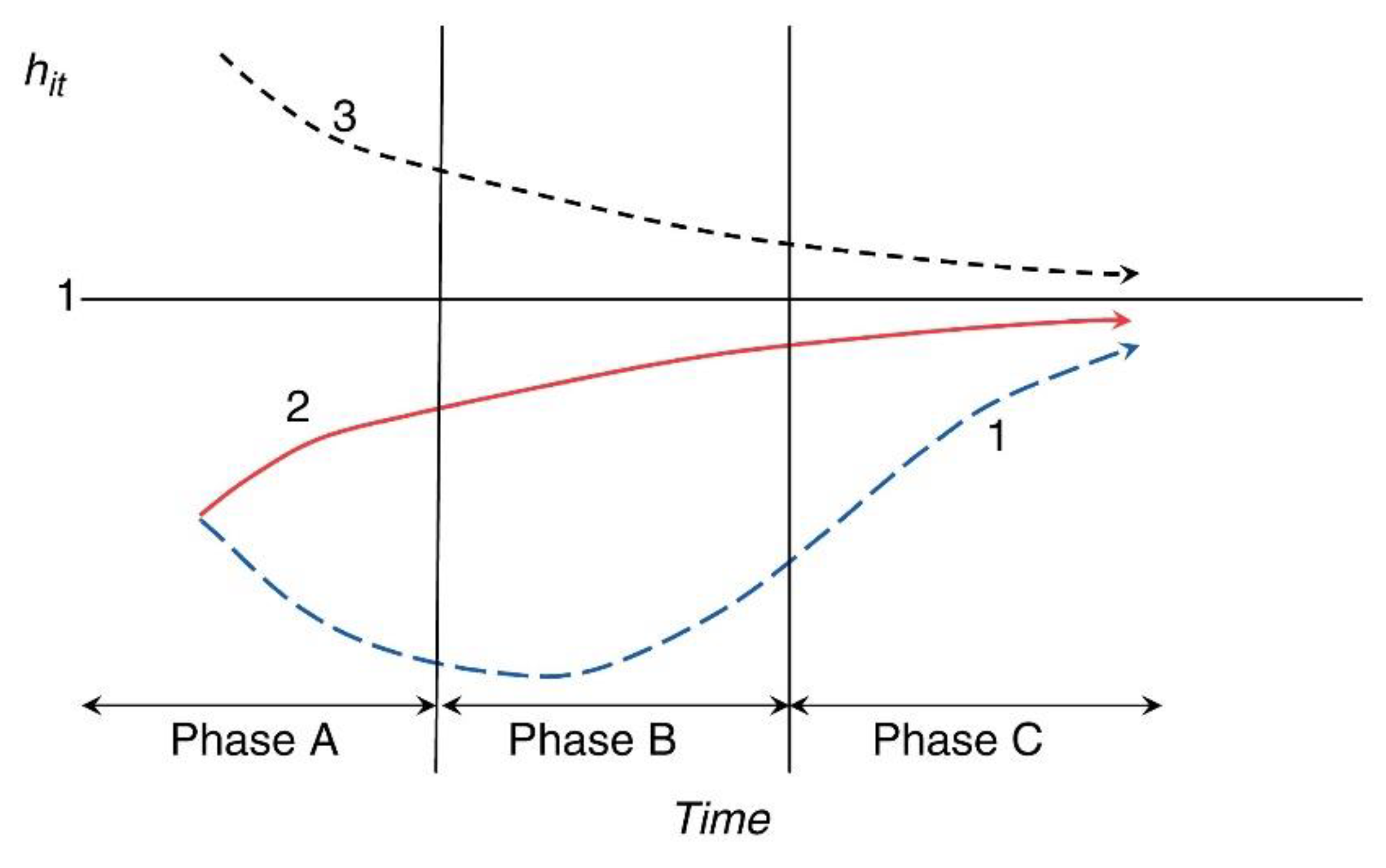
To simulate the transition parameter
δit, the relative transition parameter
hit is constructed through the following equation:
where
hit denotes the transformation path of
i economic unit compared with the cross-sectional average level. Hence, the common growth path element is eliminated, because the method calculates individual economic behaviors in relation to other economic units. Furthermore, this approach allows one to estimate the distance of unit
i from the common growth path
μt. Under convergence conditions, all economic units followed the same transformation path; when
t → ∞,
hit → 1. The cross-sectional variance of
hit can be expressed as
, which shall converge to 0. When convergence does not occur,
Vt may be positive and indicate the presence of classic convergence clubs.
To construct the null hypothesis of the economic growth convergence, Phillips and Sul [
6] presented a semi-parametric model as follows:
where
δi is constant,
σi is the heterogeneity degree parameter,
ξit is iid (0,1) across
i but weakly dependent over
t,
L(
t) is a slowly varying function for which
L(
t) → ∞ as
t → ∞, and
α is the decline rate. This formula guarantees that
δit converges to
δi for all
α ≥0. Hence, it can be seen as a null hypothesis.
The convergence null hypothesis can be expressed as follows:
And it is tested against the alternative for all i or . Therefore, even if the other methods fail, the log t test can be used to identify economic behaviors that were traditionally thought to be divergent.
Phillips and Sul [
6] presented a limiting format of cross-sectional variance
hit based on Equation (6):
Therefore, the convergence test regression equation can be written as
where
. According to the Monte Carlo simulation, the
L(
t) = log
t and
r = 0.3 setting when the sample scope
T is smaller than 50 is quite reasonable. The critical parameter
b is associated with
α. They indicated that the fitted value of log
t is
(where
is the estimated value of
α in
H0)
. A unilateral
t-test robust to heteroskedasticity and autocorrelation (HAC) is used to test the inequality of null hypothesis
. If
(the conventional robust
t statistic for the coefficient
, significant at the 5% level), the null hypothesis of convergence is rejected.
However, rejecting the null hypothesis of convergence does not mean that there is no convergence in the subgroups of the panel, because different situations can be met. For example, it is still possible that the presence of convergence clusters in the full panel follow steady-state growth paths [
6]. Hence, it is necessary to identify whether there are convergence clubs in the full panel. In this regard, Phillips and Sul [
6] suggested the following steps to identify the convergence clubs.
Step 1: Sample units (counties) are processed following reversed order in the full panel.
Step 2: Selecting the first k highest counties (log GDP per capita) in the panel to compose the core group Gk for some N > k ≥2, we then perform the log t regression and calculate the convergence test statistic for the core group Gk. Based on a standard subject to , the number of counties in the core group is determined by maximizing tk over k. Condition can help to ensure that the null hypothesis of convergence is valid for each k. If all counties were assigned a single convergence club, then the number of convergence clubs is N. In contrast, if there are two or more convergence clubs, the cluster will have a size smaller than N. If is not supported for k = 2, then the highest counties in the core group can be excluded from each subgroup, and new subgroups are formed. This procedure can be implemented again and again to meet the condition. If the condition is not supported for all such sequential pairs, then we reason that those counties were divergent.
Step 3: We set as a complemental group to the core group , brought one of the remaining counties in at a time to the k* members of the core group , and performed the log t regression. If , the counties were contained in the convergence club, where c is some chosen critical value ( represents the t-statistic for this regression). Usually, we used the Monte Carlo method to identify the choice of the critical value. This step was repeated for the rest of counties and shaped the first sub-convergence club. We needed to operate the log t regression for this first sub-convergence club and make sure that for the entire group. If not, the critical value, c, needed to be raised to improve the identifying ability of the log t test, and we repeated this procedure until the emergence of first sub-convergence group.
Step 4: We shaped a sub-group for all counties for which in Step 3 and performed the log t regression for this sub-group to verify whether and this cluster converged. In that case, we could infer that there were two convergent clubs in the panel. If not, we continued to perform Steps 1–3 on this sub-group to ensure whether there was a smaller sub-group that shaped a convergence club. If there was no k in Step 2 for which , it drew the conclusion that the rest of the counties were divergent.
Convergence club identification is realized through GAUSS9.0. GAUSS codes were sourced from Phillips and Sul [
2]. The panel logarithmic GDP per capita of 2286 counties was an input data to identify the economic growth convergence clubs.
3.2. Dynamic Spatial Ordered Probit Regression Model
The dynamic spatial ordered probit regression model that considers spatial autocorrelation extends the scope of the existing research [
36,
41]. Wang [
39] and Wang and Kockelman [
38] discussed the settings and estimation methods of the DSOP model in detail.
The DSOP model settings are as follows:
where
i is the clubs (
I = 1,…,
M),
k denotes individual counties inside the clubs (
k = 1,…,
ni), and
t is the time period. In another expression, there are
M counties/neighborhoods, each of which includes
ni observations, and the observation total is
.
λ is the time autocorrelation estimated coefficient. Each unit is observed over
T time period, producing a total observation number of
NT.
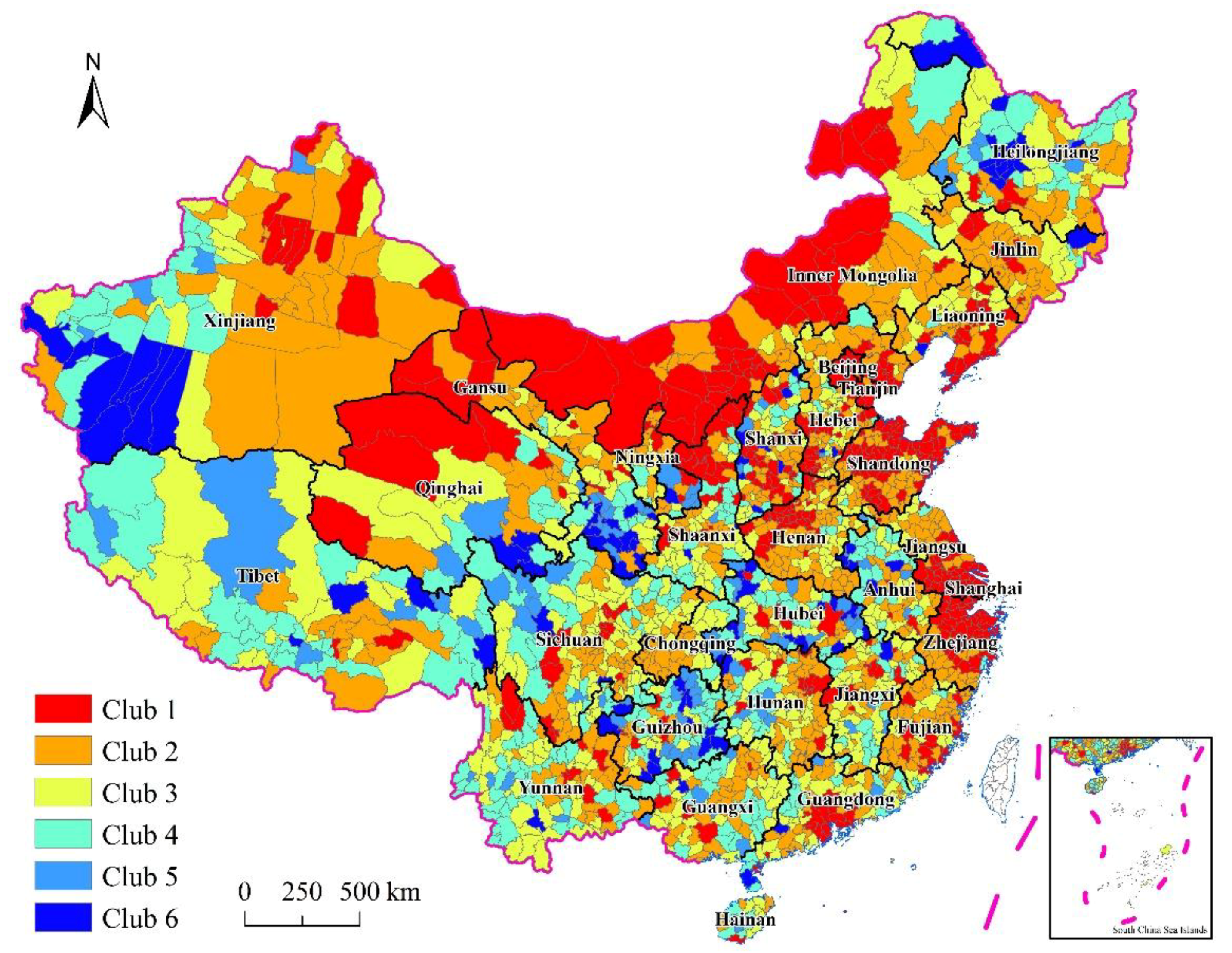
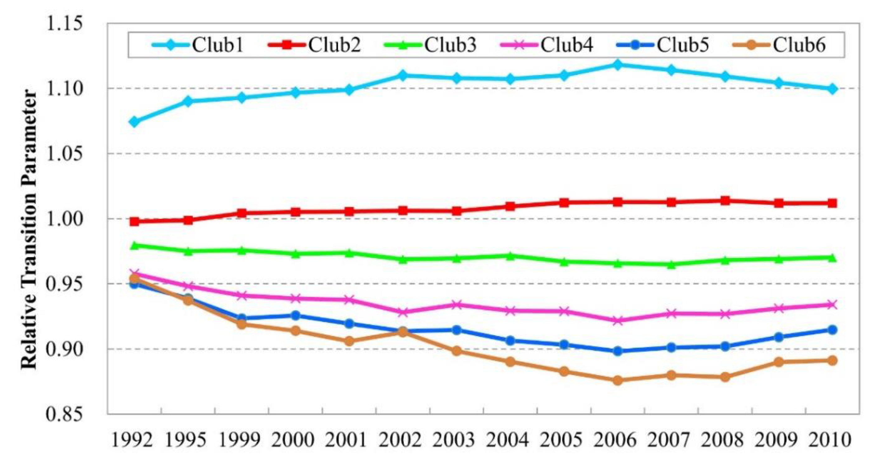
Uikt is the potential response variable (unobserved) in this paper. The range of values was from 1 to 6, corresponding to 6 identified convergence clubs. However, the sixth club included only 94 counties, thus, we merged clubs 5 and 6 into one club. The final response variables ranged from 1–5 for unit
k from county
i during time
t.
Uikt−1 is one period lagged, dependent variables of the unobserved dependent variable. The residual contains two parts,
θi, which absorbs all common yet random elements for observations with county
i, while the rest of the random component is caught by individual effect
εik, which is the heteroskedasticity with variance
vi (i.e., var (
εik) =
vi). After the
Uikt−1 were controlled, the error terms are correlated and identically distributed.
Xikt is a
Q × 1 vector of independent variables, and
β is a series of corresponding estimated parameters. In this paper, the explanatory variables include the labor participation rate (LABOR), the investment in fixed assets per capita (LNFIX), human capital (LNHUM), population density (LNDEN), and the proportion of the added value of the secondary industry in GDP (IND).
These settings reflect the spatial autocorrelations with counties. A spatial autocorrelation state can be represented as follows:
where spatial weight
wij represents spatial contiguity, which can be calculated from the adjacency or distance between counties. The degree of neighboring impact is represented by the spatial effect parameter
ρ.
ui aims to absorb any regional effects, and it is supposed to be iid normally distributed, with a mean of zero and a common variance of
σ2. Therefore, the spatial effect vector can be written as follows:
The regional effect vector will be a function of the weight matrix
W, which has zero on its diagonal and is composed of purely exogenous elements
wij, as follows:
For an ordered probit, the observed response variable,
yikt, can be expressed as follows:
The observed variable is a censored form of the latent variable, and the possible outcomes are integers between 1 and
S (In this paper,
S = 5, corresponding to the number of identified convergence clubs). The latent variable
Uikt can change within the unknown boundaries
;
γ0 tends to be an infinite negative, whereas
γS tends to be an infinite positive. If the constant term is involved in the explanatory variables,
γ1 also is normalized to equal 0. The probabilities of these
S outcomes can be expressed as follows:
where Ф (•) is the cumulative distribution function of the standard normal distribution.
The resulting likelihood function can be expressed as follows as follows:
where
y,
U, and
γ are the vector of
yikt,
Uikt, and
γs, respectively.
ϑ (
A) is an indicator function that equals 1 when event
A is true (and 0 otherwise).
The DSOP model estimation method functions within the Bayesian framework, in which each parameter corresponds to prior and posterior distributions. The posterior distribution is calculated using the Markov chain Monte Carlo method. Wang [
39] describes this estimation method in detail.
Detailed calculations of the convergence club influencing factors were performed through Matlab 2012a, and the codes were developed by Wang and Kockelman [
38] and Wang [
39].
3.3. Sample Data and Preliminary Processing
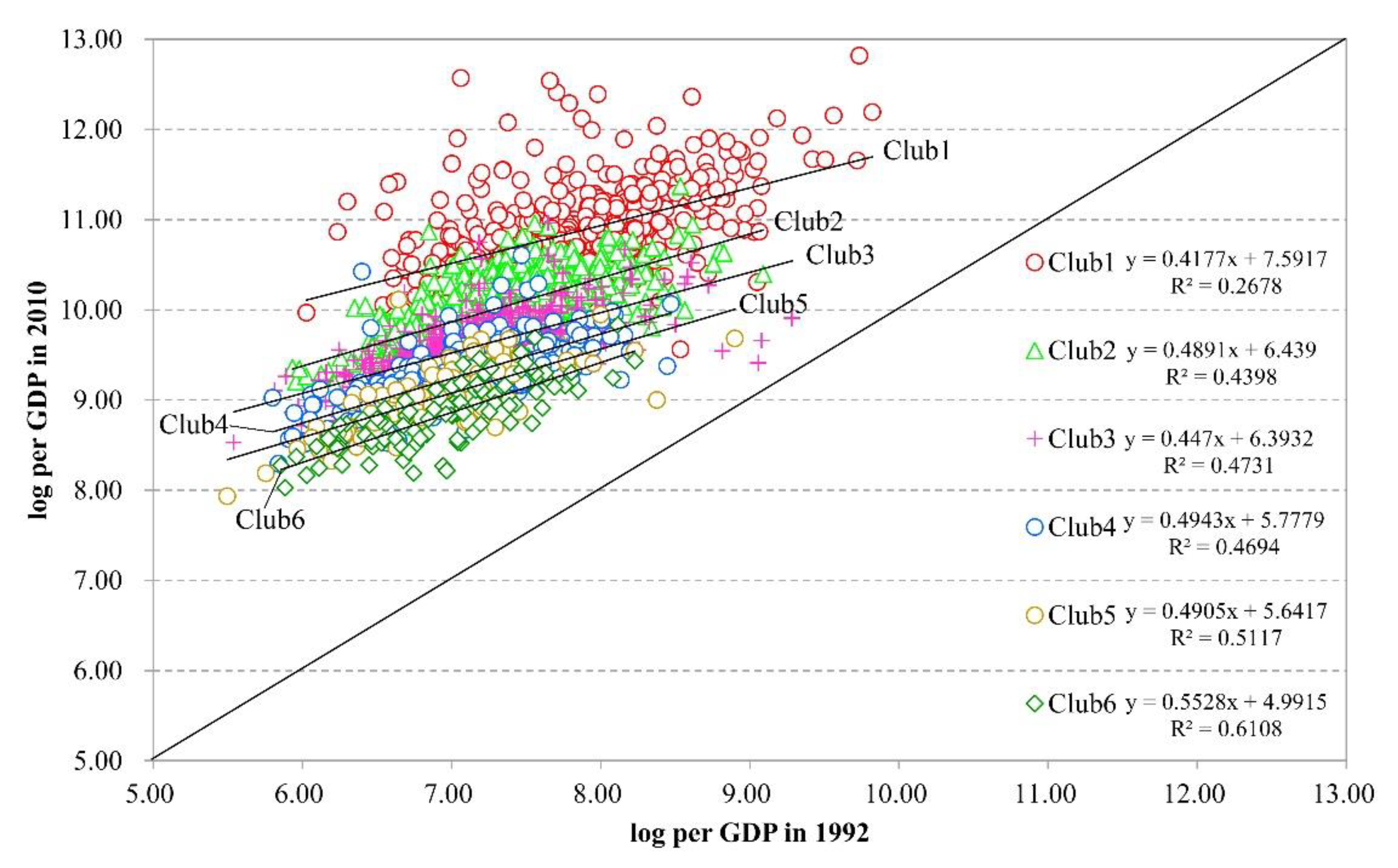
A county is a basic administrative unit of China, used to organize economic activities and administrative management, to support economic life, social life and cultural life, to connect the rural–urban interflow, and to promote rural economic development and industrialization. In fact, the stabilization and development of counties is a basis to boost the political stability, social progress, and economic prosperity of China. Using the county as a basic unit provides a finer analysis of convergence clubs compared with using a prefecture or province. Moreover, using the county as a basic unit helps investigate the inner regional equality within prefectures or provinces. There are three administrative units at the county level in China: the county (including autonomous counties), the county-level city, and the urban district. Data on counties and county-level cities were primarily derived from the China Statistical Yearbook for Regional Economy (2002–2011) and Social and Economic Statistical Yearbook of China’s County and City (2000–2011). Data for 1992, 1995, and 1999 were primarily drawn from the 2000 Statistical Yearbook. Because the China Statistical Yearbook for Regional Economy (2002–2011) does not include urban district data, these data were primarily derived from the China City Statistical Yearbook (1993–2011). Missing data for specific years and regions were supplemented using statistical yearbooks of various provinces (including districts and directly controlled municipalities from 1993–2011). Following basic data and data accessibility requirements, we constructed a socioeconomic database for Chinese counties for 1992–2010 (for data prior to 2000, only data for 1992, 1995, and 1999 were relatively complete for statistical reasons) that accounts for 2286 county units. The reason for choosing 1992 as the start of the study period is mainly that the socialist market economy system began to develop in China in 1992. Another reason is that China started publishing the county-level statistical data in 1992.
To examine the regional differences in the influencing factors behind the formation of convergence clubs, we used China’s four regions as our regression analyses sample to explore influencing factor effects on different regions. According to the classification methods of the National Bureau of Statistics of China (NBSC), the four main regions are defined as follows: the eastern region covers (580 sampled cities and counties) Beijing, Tianjin, Hebei, Shandong, Jiangsu, Zhejiang, Shanghai, Fujian, Guangdong, and Hainan; the central region covers (573 sampled cities and counties) Shanxi, Henan, Anhui, Hubei, and Hunan, Jiangxi; the western region covers (951 sampled cities and counties) Inner Mongolia, Shaanxi, Ningxia, Gansu, Chongqing, Sichuan, Guizhou, Yunnan, Guangxi, Qinghai, Tibet, and Xinjiang; and the northeastern region covers (182 sampled cities and counties) Liaoning, Jilin, and Heilongjiang.
Here, five explanatory variables, including the labor participation rate (LABOR), the investment in fixed assets per capita (LNFIX), the human capital (LNHUM), the population density (LNDEN), and the proportion of the added value of the secondary industry in GDP (IND), are used as input data to estimate the effects of these variables on the formation of convergence clubs. LABOR is a variable used to investigate the condition of the labor participation rate (%) in the entire society. The natural logarithm of the investment in fixed assets per capita (LNFIX) represents the investment level of each county. LNHUM reflects human capital levels, using the natural logarithm of the enrollment in regular secondary schools as the proxy variable. The natural logarithm of population density (LNDEN) variable is used to investigate the effects of population aggregation. IND is the proportion of the added value of the secondary industry in GDP (%) (see
Table 1 for detailed description).
Table 2 lists the descriptive statistics results for six key variables.
Graphic data were primarily drawn from the National Geomatics Center of China (NGCC,
http://ngcc.sbsm.gov.cn) and the data sharing infrastructure of Earth System Science (www.geodata.cn). Due to continuous changes in administrative divisions, we needed to adjust administrative units. To ensure the consistency of the counties over several years, a backtracking method, in which administrative division codes were reviewed from the final year to the first year, was applied. To ensure regional continuity over time and to render the data order consistent with the basic characteristics of panel data, we compared the characteristics of counties for each year and adjusted counties that experienced changes. Because GDP is a current price measure that must be deflated to improve the accuracy of the data, we deflated the county GDP index for all of the studied years to the level recorded in 1992.
Basic spatial weight matrix calculation data included latitude and longitude coordinates for the central points of the counties listed on a nationwide county map provided by the NGCC. Coordinate information extraction and application was realized through ESRI ArcGIS 10.1. We used the Matlab 2012a platform to convert coordinate information into a spatial weight matrix via xy2cont coding (
http://www.spatial-econometrics.com/), finally obtaining a 2286 × 2286 adjacency matrix.


