A Novel Stochastic Two-Stage DEA Model for Evaluating Industrial Production and Waste Gas Treatment Systems

Abstract

In recent decades, the high-speed development in China has caused serious air pollution in China. The present paper proposes a stochastic data envelopment analysis (DEA) model based on a general two-stage structure with comprehensively considering the randomness in both desirable and undesirable outputs to calculate the environmental efficiency of the industry system. The new proposed model is more applicable to practical system, and is applied to evaluate the performance of production and waste gas treatment in the industrial sector for China’s regions along the “One Belt and One Road” in 2015. The results show that about half of the regions along “One Belt and One Road” in China are inefficient, where the performance on waste gas treatment is significantly worse than that of industrial production. Further, the managers should take different strategies for efficiency improvement in different areas because of the obvious differences in efficiency scores, in which the regions in the southeast area should pay more attention to improving waste gas treatment efficiency while that in the northwest area need to focus on industrial production efficiency.

1. Introduction

China’s industry section has gained remarkable development during the past several decades, which has surpassed the United States to become the world’s largest industrial producer. However, the environmental efficiency in China’s industry section cannot match its size. As China’s industrialization deepens, the problem of air pollution is gradually increasing, which has caused serious health problems in the whole country [1]. China has become the country with the most serious air pollution all around the world based on the results in “2016 Yale environmental performance index report”. Finally, Langrish et al. [2] report that air pollution has killed about 3 million Chinese people and cut lifespan by about 5.5 years in 2012. China’s government has done a lot of work to release the air pollution by introducing some important laws and regulations, such as “Air Pollution Prevention and Control Action Plan (2013)” and “The People’s Republic of China on the prevention and control of air pollution (2015)”. In the “China Thirteenth Five Year Plan (2016–2020)”, the Chinese government plan to significantly improve air quality. It is not easy to release air pollution problem of China’s areas in the context of high-speed economic development.

“One Belt and One Road” is a national cooperation initiative proposed by the Chinese government. With the advance of the “One Belt and One Road” strategy in China, the areas along “Belt and Road” can gain new opportunities for economic development. Many scholars research the development of Chinese regions along “Belt and Road”, such as the health resource allocation [3], the urban infrastructure utilization [4], regional logistic [5] and green economy development [6]. However, few study focuses on analyzing the air pollution problem caused by economic development for these areas. Improving the efficiency of industrial production is considered an important way to reduce the use of resources and emission of air pollution [7].

The main objective of this paper is to accurately measure the performance of production and waste gas treatment in the industrial sector for China’s regions along the “One Belt and One Road”. Considering the uncertainty of input and output variables, a novel non-radial stochastic two-stage DEA (Data Envelopment Analysis) model is constructed. From individual provinces and region perspective, environmental efficiency under different risk attitude is carefully analyzed. The remainder of the paper is organized as follows. Section 2 reviews the literature on environmental efficiency. Section 3 proposes a stochastic two-stage DEA model and converts it into an equivalent deterministic model. Section 4 provides an empirical analysis of the industrial production and waste gas treatment of Chinese regions along the “One Belt and One Road”. Finally, conclusions are provided in Section 5.

2. Literature Review

Efficiency measurement is an important task in management to show the past accomplishments of a unit but also identifies targets for future development [8]. As one of the most popular tools for measuring efficiency, Data Envelopment Analysis is widely used to evaluate the efficiency score in all fields because it does not need any information of input and output variables [9]. Based on the input–output indicator value of decision-making units (DMUs), DEA judges the efficiency of these DMUs through linear programming and constructs a production frontier according to efficient DMUs. The efficiency value of inefficient DMU is determined by its distance from the DMU to the production frontier. Since the birth of the first model, DEA has made significant progress in both theory and application.

Environmental efficiency is formally proposed by the World Economic Council for Sustainable Development, as mentioned by Desimone and Popoff [10], which means the economic value of unit environmental load. Competitive advantage in environmental efficiency will be a norm for any entity [11]. In recent years, environmental performance evaluation has attracted increasing interest since they are considered a crucial approach to save energy, reduce greenhouse gas emissions, protect the environment and mitigate global climate change [12].

As the largest developing country in the world, China has significant environmental, human health, and social problems due to rapid economic development [13,14]. DEA models have frequently been used to calculate the environmental efficiency of the different domains in China. For example, Bian and Yang [15] establish the Shannon-DEA procedure to assess the environmental efficiency of 30 provinces. Distinguishing strong and weak disposability of different undesirable outputs, Piao et al. [16] assess the environmental efficiency and the dynamic change trend of 30 provinces in China. Wu et al. [17] propose both static and dynamic energy efficiency performance indexes based on the DEA model to calculate the environmental efficiency performance of the industry section in 28 Chinese provinces. Based on a slack-based measure DEA model with nonseparable bad output and weights determined by the coefficient of variation method, He et al. [18] study the comprehensive environmental efficiency of socioeconomic sectors in China. Adopting a non-radial DEA model, Kang et al. [19] examine the environmental efficiency and investment strategy of China’s manufacturing industry. Dividing China’s iron and steel industry into five processes: sintering, coking, ironmaking, steelmaking, and steel rolling, Wang et al. [20] compare the environmental efficiency of different DEA models in 54 iron and steel enterprises. After constructing a new enhanced Russell measure (ERM) model, An et al. [21] analyze the environmental efficiency of thermal power enterprises in Anhui Province of China. Based on an improved SBM model and ML index, An et al. [22] measures the energy and environmental efficiency of the Xiangjiang River basin cities in Hunan Province of China.

However, relatively few studies focus on evaluating air pollution in China. Xie et al. [23] use the DEA model to measure air pollution in China by using SO2 to scale air problems. Sueyoshi and Yuan [24] believe incorporate PM 2.5 and PM 10 as undesirable outputs to scaling air pollution based on DEA models. Zhou et al. [1] use the composite indicator, namely the air quality index (AQI), as the only undesirable output to calculate air pollution based on DEA models. Taking industrial waste gas emission as undesirable output, Yang and Li [25] evaluate the environmental efficiency of industrial waste gas control of 39 industrial sectors in China.

In many cases, the production of DMUs may consist of a two-stage network structure with an intermediate link between two sub-stages [26]. However, the traditional DEA model regards the production process as a “black box”, and calculates the efficiency scores by considering only the initial inputs and final outputs, which is unable to provide inefficient sources [27] and biased efficiency values for DMUs [28]. The two-stage structure is widely applied to measure environmental efficiency, because the production and treatment of pollution are usually operated by different organizations in the real-world production process. DEA model has received extensive attention from scholars, and many studies have used two-stage DEA models to evaluate DMUs’ efficiency. Song et al. [29] compose DEA models based on the two-stage structure to measure the environmental efficiency score of the industry in which the pollution emitted in the first stage is used as input for the second stage. From an interest preference perspective which changes weights of two sub-stage in turn, Wu et al. [30] study the environmental efficiency of 30 provinces. Under the two-stage DEA framework, Chen et al. [31] evaluate the environmental efficiency of 30 provinces from a cooperative and non-cooperative perspective, respectively. Dividing the land transportation sector into railway transportation and road transportation, Liu et al. [32] analyze the environmental efficiency of land transportation in China-based a parallel SBM model.

Both input and output data are assumed to be deterministic in classic DEA models. However, in reality, some factors are stochastically uncertain [33]. Sengupta [34] and Land et al. [35] construct a stochastic DEA model based on chance-constrained programming to address the randomness of the input and output data, and point out that the efficiency scores based on stochastic DEA model are more realistic. Wu et al. [36] put forward a stochastic DEA model considering undesirable outputs with weak disposability to analyze Chinese provincial environment efficiency in 2009. Similarly, Jin et al. [37] present a stochastic environmental DEA model to evaluate the environmental performance of Asia Pacific Economic Cooperation (APEC) economies in 2010. Zha et al. [38] construct a non-radial stochastic DEA model to measure the environmental efficiency of different regions of China, in which the uncertainty of CO2 emission is considered. Charles and Cornillier. [39] proposed two liner models (a semi-stochastic model and a stochastic model) to study the case where the inputs are random in DEA framework. However, all the above stochastic models are based on a single-stage which is unable to deal with the complex network structure in reality. Relatively few studies address stochastic data in a two-stage DEA. Chen et al. [40] focus on the efficiency assessment of 13 major Chinese airlines from 2006 to 2014 and applied a two-stage DEA model containing undesirable intermediate outputs. Izadikhah and Saen [41] presented a new stochastic two-stage DEA model based on a two-stage structure with a shared intermediate product which can produce both desirable and undesirable outputs. There are two obvious drawbacks in the above stochastic two-stage DEA model. Firstly, both of them are radial models that means all inputs or all outputs change in the same proportion, which is not in line with reality. Secondly, although the above studies consider the undesirable output in data collection, they ignore the characteristics of undesirable output, such as weak disposability [42], which is widely used in environmental efficiency evaluation [43]. Based on a centralized control organization mechanism, Zhou et al. [44] model random variables based on a simple two-stage structure, in which all the outputs of the first stage are used as the only inputs of the second stage. However, the structure of production process in real-life world is too complex to evaluate by using existing stochastic two-stage DEA model, such as Song et al. [45], Chu et al. [46] and Bi et al. [47]. The stochastic two-stage DEA of Zhou et al. [44] is also a radial model.

The main contribution of this paper lies in two aspects. In the theoretical aspect, a general non-radial stochastic two-stage DEA model with weak disposability of undesirable intermediate outputs is proposed, which can figure out a better result in environmental efficiency evaluation. In the practical aspect, this is the first time to study the “One Belt and One Road” environmental efficiency in China by stochastic two-stage model. Specifically, We evaluate the performance of production and waste gas treatment in the industrial sector for China’s regions along the “One Belt and One Road” in 2015.

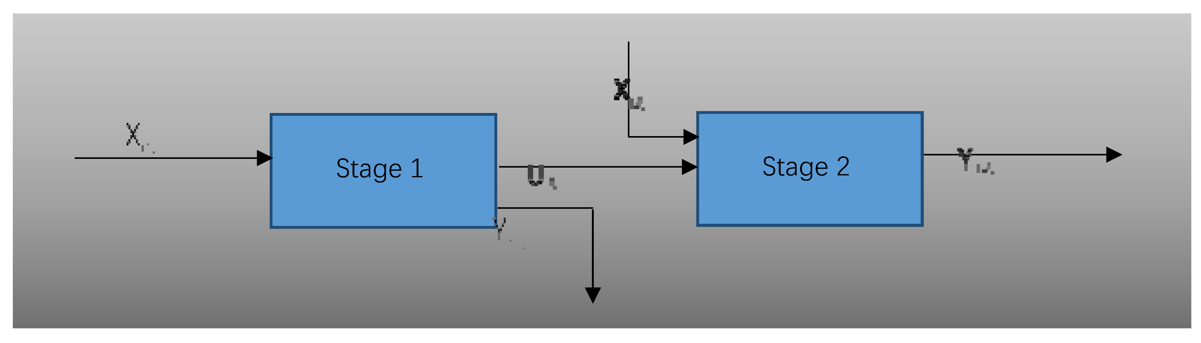
3. Proposed Stochastic Two-Stage DEA Model

Suppose that there are n DMUs, any $DM{U}_j(\mathrm{j}=1,2,\dots ,\mathrm{n})$ consumes m1 inputs $X_{i1j}(i1=1,2,\dots ,m1)$ to produce s1 desirable outputs $Y_{r1j}(r1=1,2,\dots ,s1)$ and $T$ undesirable intermediate outputs ${\tilde{U}}_{tj}(t=1,2,\dots ,T)$ in sub-stage 1. Then, sub-stage 2 disposes of the undesirable intermediate outputs ${\tilde{U}}_{tj}$ by using m2 inputs $X_{i2j}(i2=1,2,\dots ,m2)$ to obtain the s2 desirable outputs ${\tilde{Y}}_{r2j}(r2=1,2,\dots ,s2)$. As showing in Figure 1, the intermediate outputs ${\tilde{U}}_{tj}$ and final outputs ${\tilde{Y}}_{r2j}$ are random variables that represent the amount of pollutants produced and removed, while the other indexes are deterministic, such as manpower, capital investment, and benefit output.

Following the practice in Zhou et al. [44] and Bi et al. [47], the present paper ensures that the intermediate outputs used in sub-stage 2 are not greater than the output in sub-stage1. That is, $\sum _{j=1}^n{\lambda }_j^1{\tilde{U}}_{tj}\ge \sum _{j=1}^n{\lambda }_j^2{\tilde{U}}_{tj}$. Accordingly, the two-stage stochastic production possibility set is shown in formulas (1):

$$\begin{array}{l}T=\{(X1,Y1,\tilde{U},X2,\tilde{Y}2)\\ s.t.{\displaystyle \sum _{j=1}^n}{\lambda }_j^1{X}_{i1j}\le X_{i10},i1=1,2,\dots ,m1\\ \hspace{1em}{\displaystyle \sum _{j=1}^n}{\lambda }_j^1{Y}_{r1j}\ge Y_{r10},r1=1,2,\dots ,s1\\ \hspace{1em}{\displaystyle \sum _{j=1}^n}{\lambda }_j^1{\tilde{U}}_{tj}={\tilde{U}}_{t0},t=1,2,\dots ,T\\ \hspace{1em}{\displaystyle \sum _{j=1}^n}{\lambda }_j^1{\tilde{U}}_{tj}\ge {\displaystyle \sum _{j=1}^n}{\lambda }_j^2{\tilde{U}}_{tj},t=1,2,\dots ,T\\ \hspace{1em}{\displaystyle \sum _{j=1}^n}{\lambda }_j^2{X}_{i2j}\le X_{i20},i2=1,2,\dots ,m2\\ \hspace{1em}{\displaystyle \sum _{j=1}^n}{\lambda }_j^2{\tilde{Y}}_{r2j}\ge {\tilde{Y}}_{r20},r2=1,2,\dots ,s2\\ {\hspace{1em}\lambda }_j^1\ge 0,{\lambda }_j^2\ge 0\}\end{array}$$

(1)

In model (1), ${\tilde{U}}_{tj}$ and ${\tilde{Y}}_{r2j}$ are random variables, ${\mathsf{\lambda }}_j^1$ and ${\mathsf{\lambda }}_j^2$ are intensity vectors corresponding to sub-stage 1 and sub-stage 2. Constraints $\sum _{j=1}^n{\mathsf{\lambda }}_j^1{\tilde{U}}_{tj}={\tilde{U}}_{t0}$ and $\sum _{j=1}^n{\mathsf{\lambda }}_j^1{\tilde{U}}_{tj}\ge \sum _{j=1}^n{\mathsf{\lambda }}_j^2{\tilde{U}}_{tj}$ represent the weak disposability of undesirable outputs and the linkage between two stages. According to the production possibility set $\mathrm{T}$, the DEA model for calculating overall efficiency score can be obtained as model (2):

$$\begin{array}{l}E=\min \frac{1}{2}({\theta }_1+{\beta }_2)\\ s.t.{\displaystyle \sum _{j=1}^n}{\lambda }_j^1{X}_{i1j}\le {\theta }_1{X}_{i10},i1=1,2,\dots ,m1\\ \hspace{1em}{\displaystyle \sum _{j=1}^n}{\lambda }_j^1{Y}_{r1j}\ge Y_{r10},r1=1,2,\dots ,s1\\ \hspace{1em}pro\{{\displaystyle \sum _{j=1}^n}{\lambda }_j^1{\tilde{U}}_{tj}={\tilde{U}}_{t0}\}\ge 1-\alpha ,t=1,2,\dots ,T\\ \hspace{1em}pro\{{\displaystyle \sum _{j=1}^n}{\lambda }_j^1{\tilde{U}}_{tj}\ge {\displaystyle \sum _{j=1}^n}{\lambda }_j^2{\tilde{U}}_{tj}\}\ge 1-\alpha ,t=1,2,\dots ,T\\ \hspace{1em}{\displaystyle \sum _{j=1}^n}{\lambda }_j^2{X}_{i2j}\le {\beta }_2{X}_{i20},i2=1,2,\dots ,m2\\ \hspace{1em}pro\{{\displaystyle \sum _{j=1}^n}{\lambda }_j^2{\tilde{Y}}_{r2j}\ge {\tilde{Y}}_{r20}\}\ge 1-\alpha ,r2=1,2,\dots ,s2\\ {\hspace{1em}\lambda }_j^1\ge 0,{\lambda }_j^2\ge 0,0\le {\theta }_1,{\beta }_2\le 1,\forall j,i1,i2\end{array}$$

(2)

The above model (2) is a radial model in which the inputs are scale by the same proportion. Following the practices of Zhou et al. [48] and Bian et al. [15], a non-radial model stochastic DEA model is organized as follows.

$$\begin{array}{l}E=\min \frac{1}{2}(\frac{1}{m1}{\displaystyle \sum _{i1=1}^{m1}}{\theta }_1+\frac{1}{m2}{\displaystyle \sum _{i2=1}^{m2}}{\beta }_2)\\ s.t.{\displaystyle \sum _{j=1}^n}{\lambda }_j^1{X}_{i1j}\le {\theta }_{i1}{X}_{i10},i1=1,2,\dots ,m1\\ \hspace{1em}{\displaystyle \sum _{j=1}^n}{\lambda }_j^1{Y}_{r1j}\ge Y_{r10},r1=1,2,\dots ,s1\\ \hspace{1em}pro\{{\displaystyle \sum _{j=1}^n}{\lambda }_j^1{\tilde{U}}_{tj}={\tilde{U}}_{t0}\}\ge 1-\alpha ,t=1,2,\dots ,T\\ \hspace{1em}pro\{{\displaystyle \sum _{j=1}^n}{\lambda }_j^1{\tilde{U}}_{tj}\ge {\displaystyle \sum _{j=1}^n}{\lambda }_j^2{\tilde{U}}_{tj}\}\ge 1-\alpha ,t=1,2,\dots ,T\\ \hspace{1em}{\displaystyle \sum _{j=1}^n}{\lambda }_j^2{X}_{i2j}\le {\beta }_{i2}{X}_{i20},i2=1,2,\dots ,m2\\ \hspace{1em}pro\{{\displaystyle \sum _{j=1}^n}{\lambda }_j^2{\tilde{Y}}_{r2j}\ge {\tilde{Y}}_{r20}\}\ge 1-\alpha ,r2=1,2,\dots ,s2\\ \hspace{1em}{\lambda }_j^1\ge 0,{\lambda }_j^2\ge 0,0\le {\theta }_1,{\beta }_2\le 1,\forall j,i1,i2\end{array}$$

(3)

In model (3), the symbol Pro represents the probability, and the parameter $\mathsf{\alpha }$ is a certain value between 0 and 1 regarding the risk attitude of a decision-maker [38]. Then, the optimal value $E_O=1$ indicates that the DMU0 is stochastic efficient while $E_O<1$ indicates it is stochastic inefficient. ${\theta }_{i1}$ and ${\beta }_{i2}$ represent the performance of different inputs in sub-stages.

Equations (3.1) to (3.8) is a non-linear programming because of the constraint $pro\{\sum _{j=1}^n{\mathsf{\lambda }}_j^1{\tilde{U}}_{tj}\ge \sum _{j=1}^n{\mathsf{\lambda }}_j^2{\tilde{U}}_{tj}\}\ge 1-\mathsf{\alpha },\mathrm{t}=1,2,\dots ,\mathrm{T}$. It is equivalent to the following programming (4):

$$\begin{array}{l}pro\{\frac{({\displaystyle \sum _{j=1}^n}{\lambda }_j^2{\tilde{U}}_{tj}-{\displaystyle \sum _{j=1}^n}{\lambda }_j^1{\tilde{U}}_{tj})-({\displaystyle \sum _{j=1}^n}{\lambda }_j^2{\overline{U}}_{tj}-{\displaystyle \sum _{j=1}^n}{\lambda }_j^1{\overline{U}}_{tj})}{{\sigma }_t({\lambda }_j^1,{\lambda }_j^2)}\le \frac{-({\displaystyle \sum _{j=1}^n}{\lambda }_j^2{\overline{U}}_{tj}-{\displaystyle \sum _{j=1}^n}{\lambda }_j^1{\overline{U}}_{tj})}{{\sigma }_t({\lambda }_j^1,{\lambda }_j^2)}\}\ge 1-\alpha ,\\ t=1,2,\dots ,T\end{array}$$

(4)

In Equation (4), ${\overline{U}}_{tj}$ is the mean value of ${\tilde{U}}_{tj}$ and ${\sigma }_t({\lambda }_j^1,{\lambda }_j^2)$ is the standard deviation of $\sum _{j=1}^n{\lambda }_j^2{\tilde{U}}_{tj}-\sum _{j=1}^n{\lambda }_j^1{\tilde{U}}_{tj}$. Then, model (4) can be converted into model (5):

$${\displaystyle \sum _{j=1}^n{\lambda }_j^2{\overline{U}}_{tj}}-{\displaystyle \sum _{j=1}^n{\lambda }_j^1{\overline{U}}_{tj}}\le {\mathsf{\Phi }}^{-1}{\sigma }_t({\lambda }_j^1,{\lambda }_j^2),t=1,2,\dots ,T$$

(5)

In formula (5), $\mathsf{\Phi }(\alpha )$ is the accumulation function of the standard normal distribution function, and ${\mathsf{\Phi }}^{-1}(\alpha )$ is its inverse function.

Similarly, the chance constraint $pro\{\sum _{j=1}^n{\lambda }_j^2{\tilde{Y}}_{r2j}\ge {\tilde{Y}}_{r20}\}\ge 1-\mathsf{\alpha },\mathrm{r}2=1,2,\dots ,\mathrm{s}2$ can be converted into (6):

$$pro\{\frac{({\tilde{Y}}_{r20}-{\displaystyle \sum _{j=1}^n}{\lambda }_j^2{\tilde{Y}}_{r2j})-({\overline{Y}}_{r20}-{\displaystyle \sum _{j=1}^n}{\lambda }_j^2{\overline{Y}}_{r2j})}{{\sigma }_{r2}({\lambda }_j^2)}\le \frac{-({\overline{Y}}_{r20}-{\displaystyle \sum _{j=1}^n}{\lambda }_j^2{\overline{Y}}_{r2j})}{{\sigma }_{r2}({\lambda }_j^2)}\}\ge 1-\alpha ,r2=1,2,\dots ,s$$

(6)

In Equation (6), ${\overline{Y}}_{r2j}$ is the mean value of ${\tilde{Y}}_{r2j}$, ${\sigma }_{r2}({\lambda }_j^2)$ is the standard deviation of ${\tilde{Y}}_{r20}-\sum _{j=1}^n{\lambda }_j^2{\tilde{Y}}_{r2j}$, and equation (7) can be further obtained:

$${\overline{Y}}_{r20}-{\displaystyle \sum _{j=1}^n{\lambda }_j^2{\overline{Y}}_{r2j}}\le {\mathsf{\Phi }}^{-1}(\alpha ){\sigma }_{r2}({\lambda }_j^2),r2=1,2,\dots ,s2$$

(7)

The chance constraint $pro\{\sum _{j=1}^n{\mathsf{\lambda }}_j^1{\tilde{U}}_{tj}={\tilde{U}}_{t0}\}\ge 1-\mathsf{\alpha },\mathrm{t}=1,2,\dots ,\mathrm{T}$, cannot be directly converted through this method; hence, let $pro\{\sum _{j=1}^n{\mathsf{\lambda }}_j^1{\tilde{U}}_{tj}\ge {\tilde{U}}_{t0}\}\ge 1-\mathsf{\alpha },\mathrm{t}=1,2,\dots ,\mathrm{T}$ and $pro\{\sum _{j=1}^n{\mathsf{\lambda }}_j^1{\tilde{U}}_{tj}\le {\tilde{U}}_{t0}\}\ge 1-\mathsf{\alpha },\mathrm{t}=1,2,\dots ,\mathrm{T}$, using the previously described converting method, and this chance constraint can be separately converted into:

${\overline{U}}_{t0}-\sum _{j=1}^n{\mathsf{\lambda }}_j^1{\overline{U}}_{tj}\le {\mathsf{\Phi }}^{-1}(\alpha ){\sigma }_t({\lambda }_j^1)$ and $\sum _{j=1}^n{\mathsf{\lambda }}_j^1{\overline{U}}_{tj}-{\overline{U}}_{t0}\le {\mathsf{\Phi }}^{-1}(\alpha ){\sigma }_t({\lambda }_j^1)$.

At this point, model (3) can be transformed into model (8):

$$\begin{array}{l}E=\min \frac{1}{2}(\frac{1}{m1}{\displaystyle \sum _{i1=1}^{m1}}{\theta }_1+\frac{1}{m2}{\displaystyle \sum _{i2=1}^{m2}}{\beta }_2)\\ s.t.{\displaystyle \sum _{j=1}^n}{\lambda }_j^1{X}_{i1j}\le {\theta }_{i1}{X}_{i10},i1=1,2,\dots ,m1\\ \hspace{1em}{\displaystyle \sum _{j=1}^n}{\lambda }_j^1{Y}_{r1j}\ge Y_{r10},r1=1,2,\dots ,s1\\ \hspace{1em}{\overline{U}}_{t0}-{\displaystyle \sum _{j=1}^n}{\lambda }_j^1{\overline{U}}_{tj}\le {\mathsf{\Phi }}^{-1}(\alpha ){\sigma }_t({\lambda }_j^1),t=1,2,\dots ,T\\ \hspace{1em}{\displaystyle \sum _{j=1}^n}{\lambda }_j^1{\overline{U}}_{tj}-{\overline{U}}_{t0}\le {\mathsf{\Phi }}^{-1}(\alpha ){\sigma }_t({\lambda }_j^1),t=1,2,\dots ,T\\ \hspace{1em}{\displaystyle \sum _{j=1}^n}{\lambda }_j^2{\overline{U}}_{tj}-{\displaystyle \sum _{j=1}^n}{\lambda }_j^1{\overline{U}}_{tj}\le {\mathsf{\Phi }}^{-1}(\alpha ){\sigma }_t({\lambda }_j^1,{\lambda }_j^2),t=1,2,\dots ,T\\ \hspace{1em}{\displaystyle \sum _{j=1}^n}{\lambda }_j^2{X}_{i2j}\le {\beta }_{i2}{X}_{i20},i2=1,2,\dots ,m2\\ \hspace{1em}{\overline{Y}}_{r20}-{\displaystyle \sum _{j=1}^n}{\lambda }_j^2{\overline{Y}}_{r2j}\le {\mathsf{\Phi }}^{-1}(\alpha ){\sigma }_{r2}({\lambda }_j^2),r2=1,2,\dots ,s2\\ {\hspace{1em}\lambda }_j^1\ge 0,{\lambda }_j^2\ge 0,0\le {\theta }_1,{\beta }_2\le 1,\forall j,i1,i2\end{array}$$

(8)

Further suppose that random variables can be expressed as: ${\tilde{U}}_{tj}={\overline{U}}_{tj}+C_{tj}\tau$, where ${\overline{U}}_{tj}$ is the mean value, $C_{tj}$ is the standard deviation,$\tau ~N(0,1)$. ${\tilde{Y}}_{r2j}={\overline{Y}}_{r2j}+b_{r2j}\mathsf{\xi }$, where ${\overline{Y}}_{r2j}$ is the mean value, $b_{r2j}$ is standard deviation, and $\mathsf{\xi }~N(0,1)$; then, we have:

$${\sigma }_t({\lambda }_j^1,{\lambda }_j^2)=|{\displaystyle \sum _{j=1}^n{\lambda }_j^2{C}_{tj}}-{\displaystyle \sum _{j=1}^n{\lambda }_j^1{C}_{tj}}|$$

(9)

$${\sigma }_t({\lambda }_j^1)=|{\displaystyle \sum _{j=1}^n{\lambda }_j^1{C}_{tj}}-C_{t0}|$$

(10)

$${\sigma }_{r2}({\lambda }_j^2)=|{\displaystyle \sum _{j=1}^n{\lambda }_j^1{b}_{r2j}}-b_{r20}|$$

(11)

Then, model (8) can be transformed into model (12):

$$\begin{array}{l}E=\min \frac{1}{2}(\frac{1}{m1}{\displaystyle \sum _{i1=1}^{m1}}{\theta }_1+\frac{1}{m2}{\displaystyle \sum _{i2=1}^{m2}}{\beta }_2)\\ s.t.{\displaystyle \sum _{j=1}^n}{\lambda }_j^1{X}_{i1j}\le {\theta }_{i1}{X}_{i10},i1=1,2,\dots ,m1\\ \hspace{1em}{\displaystyle \sum _{j=1}^n}{\lambda }_j^1{Y}_{r1j}\ge Y_{r10},r1=1,2,\dots ,s1\\ \hspace{1em}{\overline{U}}_{t0}-{\displaystyle \sum _{j=1}^n}{\lambda }_j^1{\overline{U}}_{tj}\le {\mathsf{\Phi }}^{-1}(\alpha )|{\displaystyle \sum _{j=1}^n}{\lambda }_j^1{C}_{tj}-C_{t0}|,t=1,2,\dots ,T\\ \hspace{1em}{\displaystyle \sum _{j=1}^n}{\lambda }_j^1{\overline{U}}_{tj}-{\overline{U}}_{t0}\le {\mathsf{\Phi }}^{-1}(\alpha )|{\displaystyle \sum _{j=1}^n}{\lambda }_j^1{C}_{tj}-C_{t0}|,t=1,2,\dots ,T\\ \hspace{1em}{\displaystyle \sum _{j=1}^n}{\lambda }_j^2{\overline{U}}_{tj}-{\displaystyle \sum _{j=1}^n}{\lambda }_j^1{\overline{U}}_{tj}\le {\mathsf{\Phi }}^{-1}(\alpha )|{\displaystyle \sum _{j=1}^n}{\lambda }_j^2{C}_{tj}-{\displaystyle \sum _{j=1}^n}{\lambda }_j^1{C}_{tj}|,t=1,2,\dots ,T\\ \hspace{1em}{\displaystyle \sum _{j=1}^n}{\lambda }_j^2{X}_{i2j}\le {\beta }_{i2}{X}_{i20},i2=1,2,\dots ,m2\\ \hspace{1em}{\overline{Y}}_{r20}-{\displaystyle \sum _{j=1}^n}{\lambda }_j^2{\overline{Y}}_{r2j}\le {\mathsf{\Phi }}^{-1}(\alpha )|{\displaystyle \sum _{j=1}^n}{\lambda }_j^1{b}_{r2j}-b_{r20}|,r2=1,2,\dots ,s2\\ {\hspace{1em}\lambda }_j^1\ge 0,{\lambda }_j^2\ge 0,0\le {\theta }_1,{\beta }_2\le 1,\forall j,i1,i2\end{array}$$

(12)

In model (12), a lower $\alpha$ indicates that the decision-maker has more confidence in the evaluated DMU and assumes less risk. In most cases, the risk is limited, especially for decision-makers of city and provincial governments. Therefore, this paper follows the practice of Zhou et al. [44] and lets the value of $\alpha$ not exceed 0.5.

Based on this assumption, if $\alpha \le 0.5$, then ${\mathsf{\Phi }}^{-1}(\alpha )\le 0$. Therefore, $\sum _{j=1}^n{\mathsf{\lambda }}_j^2{\overline{U}}_{tj}-\sum _{j=1}^n{\mathsf{\lambda }}_j^1{\overline{U}}_{tj}\le {\mathsf{\Phi }}^{-1}(\alpha )|\sum _{j=1}^n{\mathsf{\lambda }}_j^2{C}_{tj}-\sum _{j=1}^n{\mathsf{\lambda }}_j^1{C}_{tj}|$ is equivalent to $-{\mathsf{\Phi }}^{-1}(\alpha )|\sum _{j=1}^n{\mathsf{\lambda }}_j^2{C}_{tj}-\sum _{j=1}^n{\mathsf{\lambda }}_j^1{C}_{tj}|\le \sum _{j=1}^n{\mathsf{\lambda }}_j^1{\overline{U}}_{tj}-\sum _{j=1}^n{\mathsf{\lambda }}_j^2{\overline{U}}_{tj}$.

This constraint can be further converted into: $-(\sum _{j=1}^n{\mathsf{\lambda }}_j^1{\overline{U}}_{tj}-\sum _{j=1}^n{\mathsf{\lambda }}_j^2{\overline{U}}_{tj})\le -{\mathsf{\Phi }}^{-1}(\alpha )(\sum _{j=1}^n{\mathsf{\lambda }}_j^2{C}_{tj}-\sum _{j=1}^n{\mathsf{\lambda }}_j^1{C}_{tj})\le \sum _{j=1}^n{\mathsf{\lambda }}_j^1{\overline{U}}_{tj}-\sum _{j=1}^n{\mathsf{\lambda }}_j^2{\overline{U}}_{tj}$.

Similarly, the remaining three absolute value limitations can be converted to corresponding inequality constraints. The final equivalent transformation model, which is a linear programming problem, is shown in model (13):

$$\begin{array}{l}E=\min \frac{1}{2}(\frac{1}{m1}{\displaystyle \sum _{i1=1}^{m1}}{\theta }_1+\frac{1}{m2}{\displaystyle \sum _{i2=1}^{m2}}{\beta }_2)\\ s.t.{\displaystyle \sum _{j=1}^n}{\lambda }_j^1{X}_{i1j}\le {\theta }_{i1}{X}_{i10},i1=1,2,\dots ,m1\\ {\displaystyle \sum _{j=1}^n}{\lambda }_j^1{Y}_{r1j}\ge Y_{r10},r1=1,2,\dots ,s1\\ -{\mathsf{\Phi }}^{-1}(\alpha )({\displaystyle \sum _{j=1}^n}{\lambda }_j^1{C}_{tj}-C_{t0})={\overline{U}}_{t0}-{\displaystyle \sum _{j=1}^n}{\lambda }_j^1{\overline{U}}_{tj},t=1,2,\dots ,T\\ -{\mathsf{\Phi }}^{-1}(\alpha )({\displaystyle \sum _{j=1}^n}{\lambda }_j^1{C}_{tj}-C_{t0})={\displaystyle \sum _{j=1}^n}{\lambda }_j^1{\overline{U}}_{tj}-{\overline{U}}_{t0},t=1,2,\dots ,T\\ {\displaystyle \sum _{j=1}^n}{\lambda }_j^1{\overline{U}}_{tj}-{\overline{U}}_{t0}\le {\mathsf{\Phi }}^{-1}(\alpha )|{\displaystyle \sum _{j=1}^n}{\lambda }_j^1{C}_{tj}-C_{t0}|,t=1,2,\dots ,T\\ -{\mathsf{\Phi }}^{-1}(\alpha )({\displaystyle \sum _{j=1}^n}{\lambda }_j^2{C}_{tj}-{\displaystyle \sum _{j=1}^n}{\lambda }_j^1{C}_{tj})\le {\displaystyle \sum _{j=1}^n}{\lambda }_j^1{\overline{U}}_{tj}-{\displaystyle \sum _{j=1}^n}{\lambda }_j^2{\overline{U}}_{tj},t=1,2,\dots ,T\\ -{\mathsf{\Phi }}^{-1}(\alpha )({\displaystyle \sum _{j=1}^n}{\lambda }_j^2{C}_{tj}-{\displaystyle \sum _{j=1}^n}{\lambda }_j^1{C}_{tj})\ge {\displaystyle \sum _{j=1}^n}{\lambda }_j^2{\overline{U}}_{tj}-{\displaystyle \sum _{j=1}^n}{\lambda }_j^1{\overline{U}}_{tj},t=1,2,\dots ,T\\ {\displaystyle \sum _{j=1}^n}{\lambda }_j^2{X}_{i2j}\le {\beta }_{i2}{X}_{i20},i2=1,2,\dots ,m2\\ -{\mathsf{\Phi }}^{-1}(\alpha )({\displaystyle \sum _{j=1}^n}{\lambda }_j^1{b}_{r2j}-b_{r20})\le {\displaystyle \sum _{j=1}^n}{\lambda }_j^2{\overline{Y}}_{r2j}-{\overline{Y}}_{r20},r2=1,2,\dots ,s2\\ -{\mathsf{\Phi }}^{-1}(\alpha )({\displaystyle \sum _{j=1}^n}{\lambda }_j^1{b}_{r2j}-b_{r20})\ge {\overline{Y}}_{r20}-{\displaystyle \sum _{j=1}^n}{\lambda }_j^2{\overline{Y}}_{r2j},r2=1,2,\dots ,s2\\ {\lambda }_j^1\ge 0,{\lambda }_j^2\ge 0,0\le {\theta }_1,{\beta }_2\le 1,\forall j,i1,i2\end{array}$$

(13)

Obviously, when $\alpha =0.5$, model (13) is an actual deterministic model. Then, the uncertainty of the discharge capacity is no longer considered at this time. After obtaining the overall efficiency value of each DMU, the efficiency scores of sub-stage 1 and sub-stage 2 can be solved as in Equations (14) and (15), respectively:

$$E_0^1=\frac{1}{m1}{\displaystyle \sum _{i1=1}^{m1}}{\theta }_{i1}^{*}$$

(14)

$$E_0^2=\frac{1}{m2}{\displaystyle \sum _{i2=1}^{m2}}{\beta }_{i2}^{*}$$

(15)

In model (14) and (15), ${\theta }_{i1}^{*}$ and ${\beta }_{i2}^{*}$ are the optimal solutions obtained from model (13).

4. Empirical Analysis and Results

4.1. Variables Selection and Data Description

There are 18 provinces and cities in China along Belt and Road”, which can be divided into the Northeast region (Liaoning, Jilin, and Heilongjiang), the Northwest region (Xinjiang, Shanxi, Gansu, Ningxia, Qinghai, and Inner Mongolia), the Southeast region (Shanghai, Fujian, Guangdong, Zhejiang, and Hainan) and the Southwest region (Guangxi, Yunnan, Chongqing, and Tibet) (Zhang and Tong, 2016). To measure the efficiency of production stage for these 18 provinces and cities, three inputs ($X_1^1$: quantity of industrial employment, $X_2^1$: fixed assets investments and $X_3^1$: total amount of industrial energy consumption), one desirable output ($Y^1$: industrial production value) and one undesirable output (Z: Industrial waste gas produced) are used to scale the efficiency of first production stage. The undesirable output in the first stage is considered as an intermediate output between the production stage (stage 1) and the pollution treatment stage (stage 2). In the second stage, one input ($X^2:$ Annual expenditure for operation) is used to treat the undesirable output from stage 1 (z) to produce one desirable output ($Y^2$: industrial waste gas treatment). The data are collected from the 2016 China Industrial Statistical Yearbook (NBSC, 2016), the 2012–2016 China Environmental Yearbook (NBSC, 2012-2016), and the statistical yearbooks of each of the 18 provinces and cities. The statistical description of each indicator is provided in

Table 1. Statistical description of inputs and outputs.

	Variables	Min	Max	Mean	S.T
Stage 1	Labor (1,000,000 persons)	12.22	269.44	95.65	62.21
	Fixed assets investment (100 billion RMB)	11.64	1463.8	257.1	355.3
	Total industrial energy consumption (1,000,000 TCE)	9.86	175.76	74.91	48.36
	Gross industrial production (100 billion RMB)	479.22	31,539.6	7451.4	7580.8
Intermediate output	Industrial waste gas production (1,000,000 Ton)	4.15	53.18	21.59	11.94
Stage 2	Annual expenditure for operation (1,000,000 RMB)	1032.3	10,460.6	4489.2	2945.8
	Industrial waste gas removal (1,000,000 Ton)	4,04	50.60	20.48	11.33

.

4.2. Efficiency Analysis

4.2.1. Efficiency Comparison between Deterministic and Stochastic Two-Stage Models

Based on the stochastic two-stage DEA model (13), the relevant data are programmed using MATLAB software.

Table 2. Efficiency comparison between deterministic and stochastic two-stage models.

Region	$\mathbf{Deterministic}\mathbf{Model}\mathbf{Efficiency}(\mathit{\alpha }=0.5)$			$\mathbf{Stochastic}\mathbf{Model}\mathbf{Efficiency}(\mathit{\alpha }=0.05)$
	$E_0$	$E_0^1$	$E_0^2$	$E_0$	$E_0^1$	$E_0^2$
Zhejiang	0.633 (14)	0.844 (11)	0.422 (15)	1.000 (1)	1.000 (1)	1.000 (1)
Shanghai	0.597 (16)	1.000 (1)	0.193 (1)	1.000 (1)	1.000 (1)	1.000 (1)
Fujian	0.724 (10)	0.927 (9)	0.521 (13)	0.817 (13)	1.000 (1)	0.633 (16)
Shandong	0.628 (15)	1.000 (1)	0.256 (16)	0.693 (16)	1.000 (1)	0.386 (17)
Hainan	0.897 (5)	0.794 (12)	1.000 (1)	1.000 (1)	1.000 (1)	1.000 (1)
Guangxi	1.000 (1)	1.000 (1)	1.000 (1)	1.000 (1)	1.000 (1)	1.000 (1)
Liaoning	0.642 (12)	0.857 (10)	0.427 (14)	0.749 (15)	0.861 (13)	0.638 (15)
Jilin	0.834 (9)	1.000 (1)	0.668 (11)	0.974 (10)	1.000 (1)	0.949 (12)
Heilongjiang	0.849 (8)	0.698 (14)	1.000 (1)	0.875 (11)	0.749 (14)	1.000 (1)
Inner Mongolia	0.938 (4)	1.000 (1)	0.875 (7)	1.000 (1)	1.000 (1)	1.000 (1)
Shaanxi	0.965 (2)	0.930 (8)	1.000 (1)	1.000 (1)	1.000 (1)	1.000 (1)
Gansu	0.646 (11)	0.606 (15)	0.686 (10)	0.799 (14)	0.690 (15)	0.907 (13)
Qinghai	0.540 (17)	0.533 (17)	0.547 (12)	0.678 (17)	0.613 (17)	0.742 (14)
Ningxia	0.889 (6)	1.000 (1)	0.779 (8)	1.000 (1)	1.000 (1)	1.000 (1)
Xinjiang	0.633 (13)	0.576 (16)	0.691 (9)	0.827 (12)	0.654 (16)	1.000 (1)
Chongqing	0.962 (3)	1.000 (1)	0.925 (6)	1.000 (1)	1.000 (1)	1.000 (1)
Yunnan	0.881 (7)	0.762 (13)	1.000 (1)	1.000 (1)	1.000 (1)	1.000 (1)
Average	0.780	0.855	0.705	0.907	0.916	0.897

shows the overall and sub-stages efficiency scores of the 17 provinces and cities along the “Belt and Road” by setting $\alpha =0.5$ and $\alpha =0.05$.

Based on the efficiency scores and ranking orders in Table 2, we can find some interesting conclusions. Generally, the average efficiency scores of the industrial production stage are higher than that of the waste gas treatment stage under both stochastic and deterministic models. Regardless of the overall or the sub-stages of the system, the efficiency of every DMU under the stochastic model is not lower than under the deterministic model. Under the stochastic model, more than half DMUs (9 in 17) are efficient, while only one DMU is efficient by using the deterministic model.

Many DMUs need to improve their performance because of the poor efficiency scores based on both stochastic and deterministic models, in which the province Qinhai is the DMU with the lowest efficiency score. However, the reason of poor performance for different DMUs are different, Fujian, Guangdong, Liaoning and Jilin attain low efficiency in the waste gas treatment stage, whereas Heilongjiang, Gansu, Qinghai and Xinjiang perform poorly in the industrial production stage. Some DMUs obtain quite different efficiency scores based on different models. For example, Shanghai is efficient under the stochastic model but only gets 0.597 under the deterministic model. Similar situations have also occurred in Zhejiang and Xinjiang.

4.2.2. Sensitivity Analysis of $\mathsf{\alpha }$

Table 3. Overall efficiency of the stochastic model (13) under different $\mathsf{\alpha }.$

Region	Overall Efficiency							s.t
	$\mathit{\alpha }=0.01$	$\mathit{\alpha }=0.05$	$\mathit{\alpha }=0.1$	$\mathit{\alpha }=0.2$	$\mathit{\alpha }=0.3$	$\mathit{\alpha }=0.4$	$\mathit{\alpha }=0.5$
Zhejiang	1.000	1.000	0.738	0.738	0.737	0.735	0.633	0.144
Shanghai	1.000	1.000	1.000	0.618	0.613	0.613	0.597	0.208
Fujian	0.753	0.817	0.810	0.795	0.808	0.808	0.724	0.035
Guangdong	0.693	0.693	0.693	0.692	0.691	0.690	0.628	0.024
Hainan	1.000	1.000	1.000	1.000	1.000	1.000	0.897	0.039
Guangxi	1.000	1.000	1.000	1.000	1.000	1.000	1.000	0.000
Liaoning	0.750	0.749	0.745	0.747	0.747	0.743	0.642	0.040
Jilin	0.975	0.974	0.973	0.970	0.966	0.953	0.834	0.051
Heilongjiang	0.875	0.875	0.875	0.875	0.875	0.875	0.849	0.010
Inner Mongolia	1.000	1.000	1.000	1.000	1.000	1.000	0.938	0.024
Shaanxi	1.000	1.000	1.000	1.000	1.000	1.000	0.965	0.013
Gansu	0.803	0.799	0.794	0.789	0.764	0.763	0.646	0.055
Qinghai	0.679	0.678	0.676	0.673	0.667	0.652	0.540	0.050
Ningxia	1.000	1.000	1.000	1.000	1.000	1.000	0.889	0.042
Xinjiang	0.827	0.827	0.827	0.827	0.827	0.827	0.633	0.073
Chongqing	1.000	1.000	1.000	1.000	1.000	1.000	0.962	0.014
Yunnan	1.000	1.000	1.000	1.000	1.000	1.000	0.881	0.045
Average	0.903	0.907	0.890	0.866	0.864	0.862	0.780	-
Number of efficient DMU	9	9	8	7	7	7	1	-

reports the overall efficiency scores for every DMU under different risk attitudes $\alpha$ to analyze the sensitivity of parameter $\mathsf{\alpha }$. The last column of Table 3 shows the standard deviation of efficiency scores based on different $\alpha$, which shows the efficiency scores of all the DMUs except Guangxi change with $\alpha$. The results indicate that the randomness of the data has significant impact on the efficiency value. The overall average efficiency of the stochastic two-stage model shows an inverted “U” type change as $\alpha$ increases, and the maximum average efficiency is 0.907 when $\alpha =0.05$. For individual provinces, it is worth noting that different provinces have different efficiency change trend. So, in order to maximize environmental efficiency, different provinces and cities should carefully choose appropriate risk attitudes.

Figure 2 indicates the efficiency score of the industrial production stage for each DMU under different $\alpha$. When $\alpha \le 0.4$, the efficiency score of the industrial production stage in most DMUs remains unchanged (except for Liaoning Province, which shows irregular changes). 7 DMUs, namely Shanghai, Guangdong, Guangxi, Jilin, Inner Mongolia, Ningxia and Chongqing, keep efficient under all values, while Qinghai obtains the lowest efficiency score 0.533 when $\alpha =0.5$. As showing in Figure 3, the efficiency change of the waste gas treatment stage is more remarkable, because two random variables are used in this stage. Only 5 DMUs (Hainan, Guangxi, Heilongjiang, Shanxi and Yunnan) are efficient based on all the possibility of $\alpha$. Shanghai is the poorest performance DMU on waste gas treatment with an efficiency score of 0.193 under $\alpha =0.5$. Figure 4 describes the mean value and standard deviation of the sub-stage efficiency with different $\alpha$ values, in which we can find that the average efficiency score of air pollution stage is much lower than that of the industrial production stage.

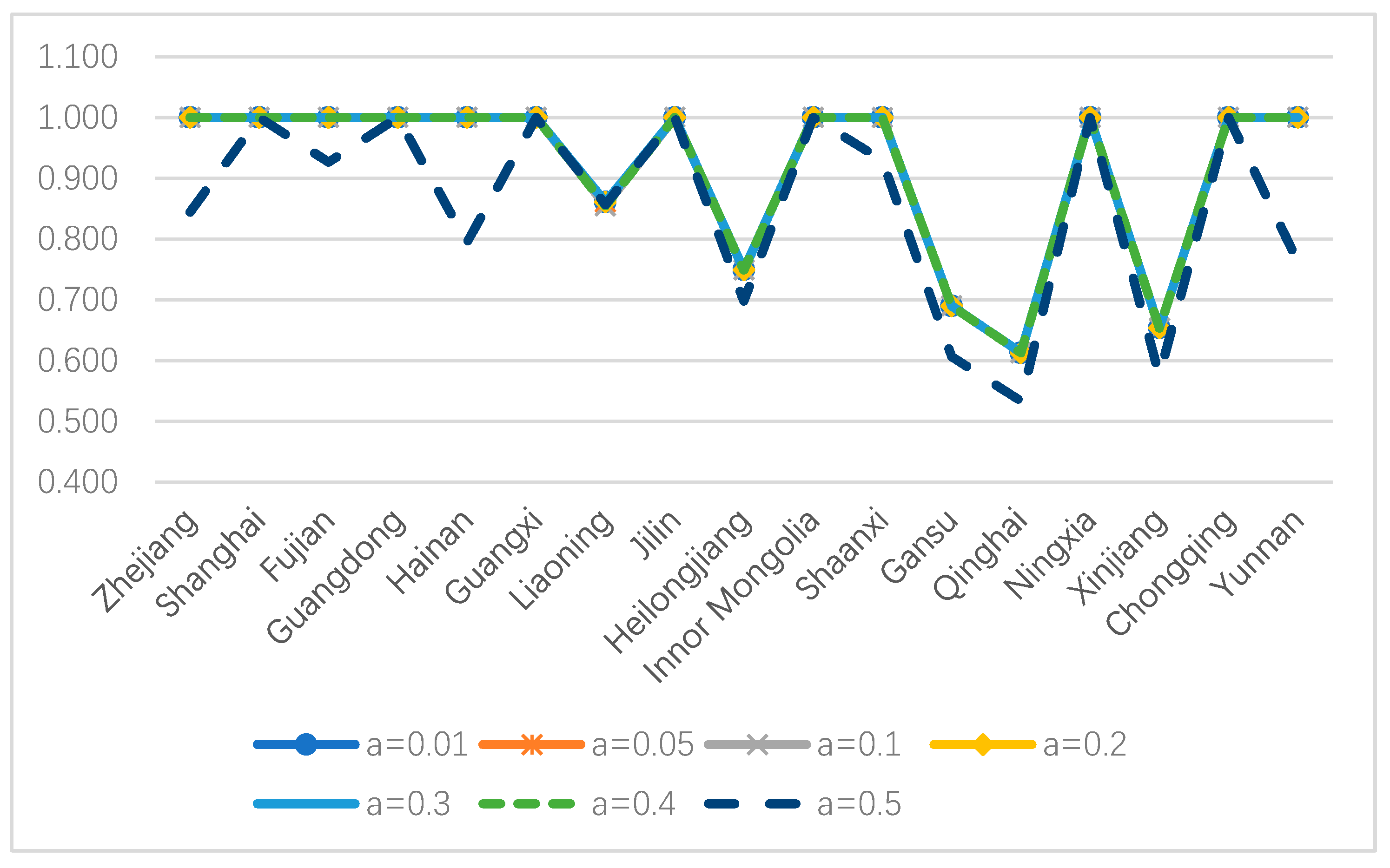
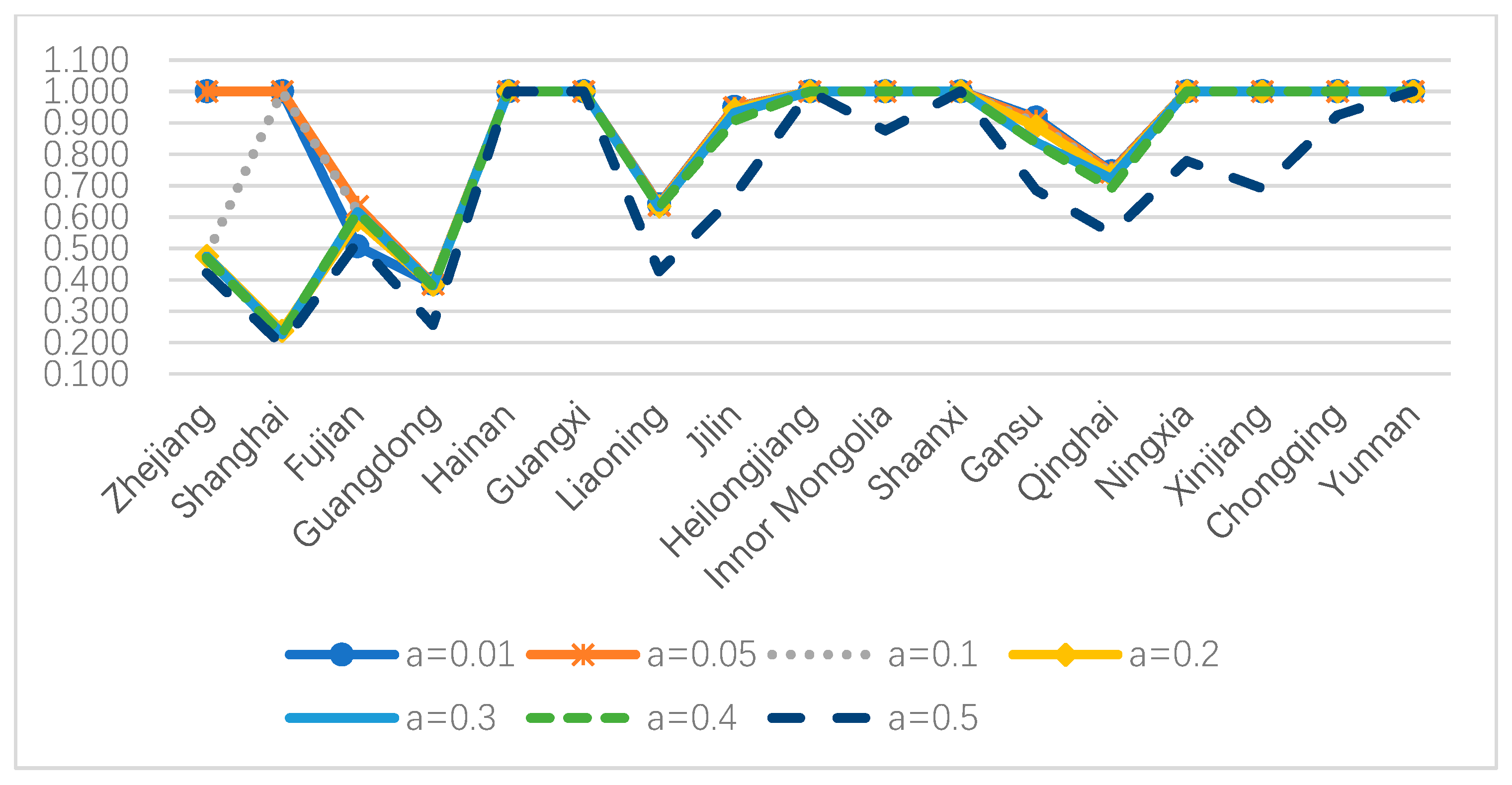
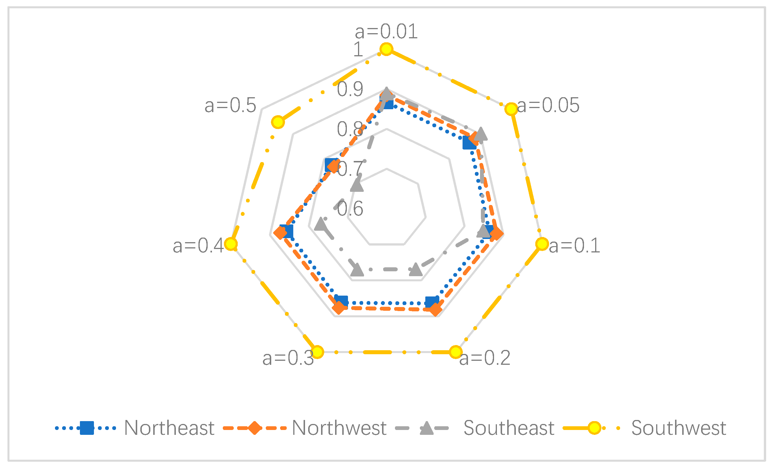
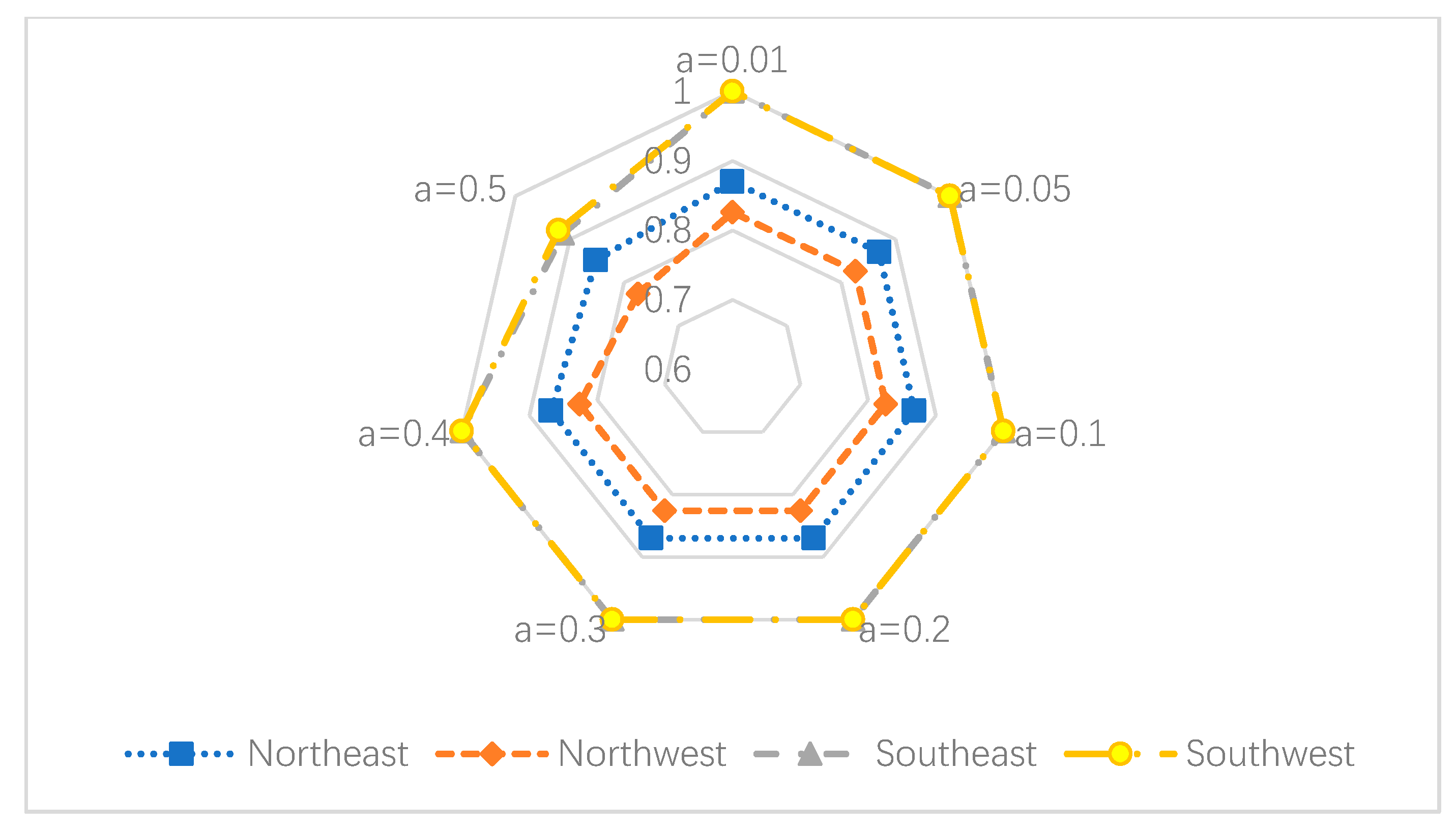
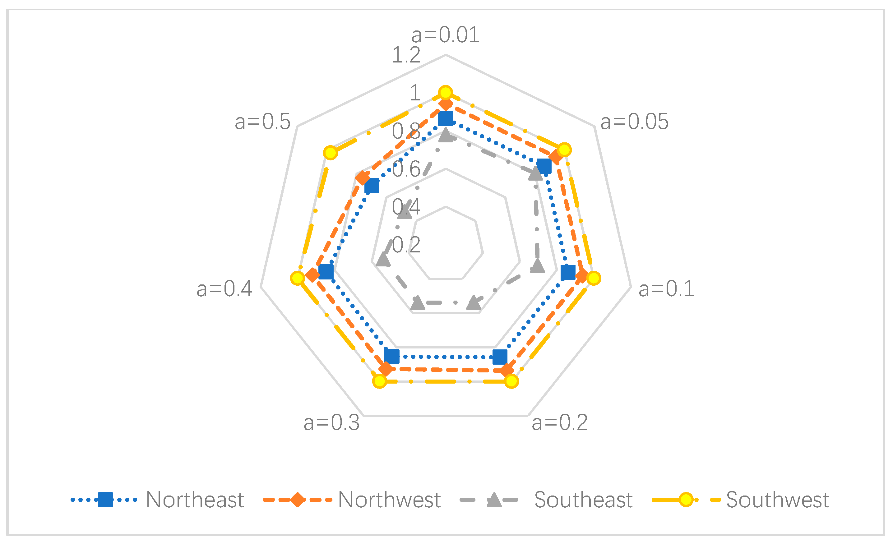
4.2.3. Evaluation from the Regional Perspective

Figure 5, Figure 6 and Figure 7 show the trends of overall and sub-stage efficiency values for different regions under different $\alpha$. Figure 5 indicates that the overall efficiency score of the southwestern region is relatively high, which only decreases slightly at $\alpha =0.5$. The northwest and northeast regions show similar trends and basically maintained overall efficiency scores at the same level, which also shows a gradual decreasing trend with the increasing of $\alpha$. Figure 6 and Figure 7 the differences in industrial production and waste gas treatment stages between regions. Southeast area performs well in the production stage but gains the lowest efficiency score in the treatment stage, while the northeast area performs much better in the treatment stage than the production stage.

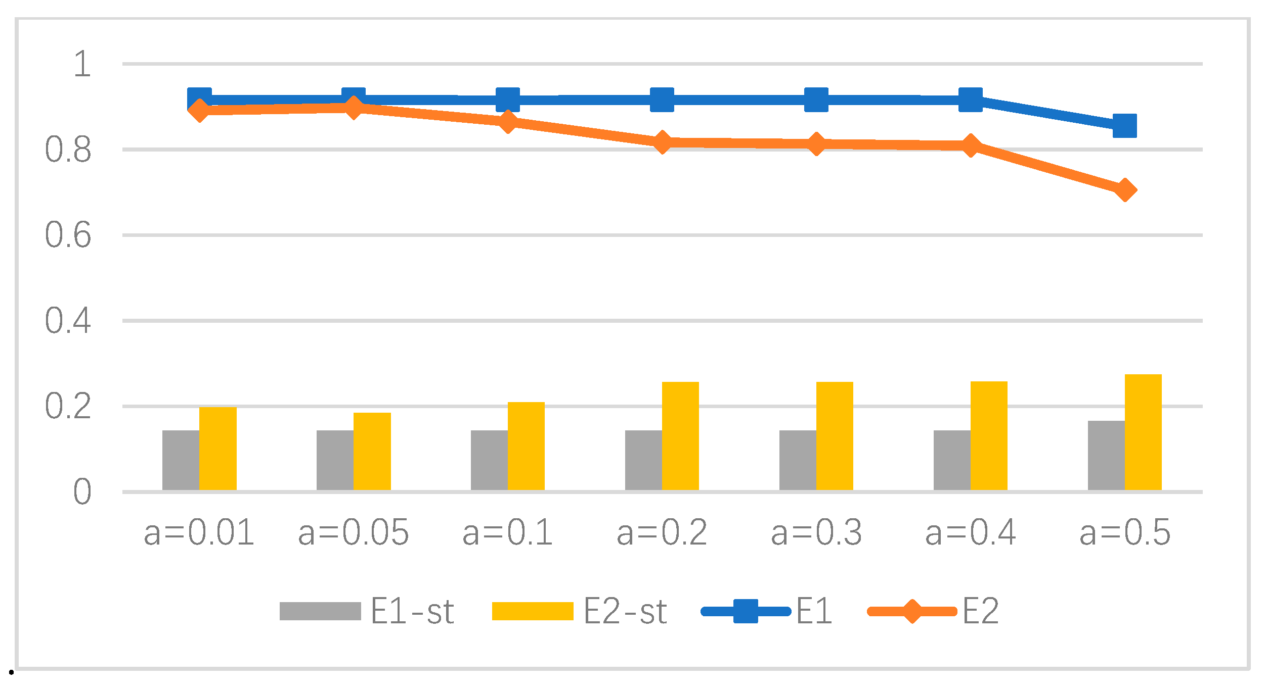
4.2.4. Efficiency Comparison between Proposed Stochastic Two-Stage Model and Corresponding Stochastic Single-Stage Model

Most of the existing studies use single-stage DEA model to calculate the efficiency score of waste gas treatment. To verify the rationality of the proposed model, the present paper provides a comparative analysis between the proposed two-stage model and single-stage stochastic DEA model.

Table 4. Efficiency of stochastic single-stage DEA model.

Region	Efficiency
	$\mathit{\alpha }=0.01$	$\mathit{\alpha }=0.05$	$\mathit{\alpha }=0.1$	$\mathit{\alpha }=0.2$	$\mathit{\alpha }=0.3$	$\mathit{\alpha }=0.4$	$\mathit{\alpha }=0.5$
Zhejiang	0.775	0.773	0.773	0.773	0.773	0.773	0.773
Shanghai	0.843	0.841	0.841	0.841	0.841	0.841	0.841
Fujian	1.000	1.000	1.000	0.954	0.952	0.950	0.947
Guangdong	1.000	1.000	1.000	1.000	1.000	1.000	1.000
Hainan	0.740	0.731	0.726	0.719	0.714	0.708	0.703
Guangxi	1.000	1.000	1.000	1.000	1.000	1.000	1.000
Liaoning	0.811	0.811	0.811	0.811	0.811	0.811	0.810
Jilin	1.000	1.000	1.000	1.000	1.000	1.000	1.000
Heilongjiang	1.000	1.000	1.000	1.000	1.000	1.000	1.000
Inner Mongolia	1.000	1.000	1.000	1.000	1.000	1.000	1.000
Shaanxi	1.000	1.000	1.000	1.000	1.000	1.000	1.000
Gansu	0.814	0.805	0.799	0.792	0.787	0.782	0.766
Qinghai	0.674	0.655	0.640	0.629	0.624	0.620	0.617
Ningxia	1.000	1.000	1.000	1.000	1.000	1.000	1.000
Xinjiang	1.000	1.000	1.000	1.000	1.000	1.000	1.000
Chongqing	1.000	1.000	1.000	1.000	1.000	1.000	1.000
Yunnan	1.000	1.000	1.000	0.935	0.914	0.895	0.871
Average	0.921	0.919	0.917	0.909	0.907	0.905	0.902
Number of efficient DMU	11	11	11	9	9	9	9

reports the efficiency score computed by single-stage stochastic DEA model, which is provided in the Appendix A. In this model, undesirable intermediate output is not considered, while all inputs and outputs in the first and second stages are used ($X^1, X^2, Y^1\mathrm{and}{\tilde{Y}}^2 \mathrm{in}$ Figure 2).

The efficiency scores under a single DEA model are shown in Table 4. By comparing with the overall efficiency under two-stage model in Table 3, one can find the two-stage model has the stronger discriminating ability on the efficiency results. First, the number of efficient DMUs under the two-stage model is smaller than that under the single-stage model by using all $\alpha$ values. Especially when $\alpha =0.5$, there are 9 efficient DMUs under the single-stage model, while only one DMU (Guangxi) is efficient under the two-stage model. Secondly, the mean efficiency score under different $\alpha$ under the two-stage model is smaller than that under the single-stage model.

5. Conclusions

In reality, available data are usually uncertain which is difficult to calculate by using the existing DEA model. Stochastic uncertainty is one of the diverse causes of uncertainty and is necessary to modeling random variables in the DEA approach. The present paper proposes a stochastic two-stage DEA model based on a general two-stage structure with considering the randomness on both desirable and undesirable variables based on both radial and non-radial forms. Subsequently, the proposed model is applied to the efficiency study of the industry section for 17 regions in China along the “One Belt and One Road” in the year of 2015. Based on the efficiency results, we find that about half of the regions along “Belt and Road” in China are inefficient on environmental efficiency in the industry section. In which, the performance of waste gas treatment is weaker than that of industrial production. Besides, similar to the results in [30] and [43] there are significant differences between the efficiency scores in different areas, where the southwest is the area with the best efficiency score while the southeast is the poorest performance area. Further, there are still differences between the performances for different stages in these areas that might guide the managers to take effective ways to improve efficiency.

The present paper also analysis the sensitivity of risk attitudes by setting different $\alpha$ values in the newly constructed models. Based on the results of sensitivity analysis, the selection of $\alpha$ is very important in the presented model and should cause significant differences to the efficiency scores in both overall efficiency and sub-stage efficiency scores. Different provinces and cities should carefully choose appropriate risk attitudes to maximize their environmental efficiency.

In the future, there are two interesting research directions. First, more complex network structures, such as a two-stage model with shared inputs and common outputs, should be extended to the sentiment of random numbers. Second, the present paper follows the practice in Zhou et al. [44] and sets $\alpha \le 0.5$ in efficiency calculation. However, the value of $\alpha$ will no longer be limited to smaller than 0.5 in some of the other research objects. How to determine the range and optimal value of parameter $\alpha$ should be discussed in the future.

References

1. Zhou, Z.; Guo, X.; Wu, H.; Yu, J. Evaluating air quality in China based on daily data: Application of integer data envelopment analysis. J. Clean. Prod. 2018, 198, 304–311. [Google Scholar] [CrossRef]
2. Langrish, J.P.; Bosson, J.; Unosson, J.; Muala, A.; Newby, D.E.; Mills, N.L.; Blomberg, A.; Sandström, T. Cardiovascular effects of particulate air pollution exposure: time course and underlying mechanisms. J. Intern. Med. 2012, 272, 224–239. [Google Scholar] [CrossRef] [PubMed]
3. Alimu, M.; Salipu, A.; Wang, Y.F.; Tang, C.Y.; Han, C.Y. A Study on the Efficiency of Medical and Health Resource Allocation in the Five Northwest Provinces and the Five Central Asian Countries against the Background of “One Belt and One Road”—An Empirical Study Based on the Three-Stage DEA Model. J. Lanzhou Univ. (Social Sci.). 2016, 4, 90–94. [Google Scholar]
4. Zhang, Q.; Tong, J.X. Analysis of Urban Infrastructure Efficiency of the Provinces and Cities on the Belt and Road Area—Based on DEA and Malmquist Index Model. Soft Sci. 2016, 30, 114–117. [Google Scholar]
5. Zhang, X.Q. Analysis on the coordinated development of regional logistics in the “One Belt and One Road”. Stat. Decis. 2016, 8, 108–110. [Google Scholar]
6. Zhang, W.B.; Deng, L.; Yin, C.B. Evaluation of Green Economy Efficiency and Analysis of Influencing Factors in Major Node Cities of “One Belt and One Road”. Inq. Econ. Issues. 2017, 11, 84–90. [Google Scholar]
7. Zhou, Z.; Wu, H.; Song, P. Measuring the resource and environmental efficiency of industrial water consumption in China: A non-radial directional distance function. J. Clean. Prod. 2019, 240, 118169. [Google Scholar] [CrossRef]
8. Kao, C. Efficiency measurement and frontier projection identification for general two-stage systems in data envelopment analysis. Eur. J. Oper. Res. 2017, 261, 679–689. [Google Scholar] [CrossRef]
9. Charnes, A.; Cooper, W.; Rhodes, E. Measuring the efficiency of decision making units. Eur. J. Oper. Res. 1978, 2, 429–444. [Google Scholar] [CrossRef]
10. Desimone, L.D.; Popoff, F. Eco-efficiency: the business link to sustainable development. Crop. Environ. Strategy. 2000, 1, 220–221. [Google Scholar]
11. Rashidi, K.; Saen, R.F. Measuring eco-efficiency based on green indicators and potentials in energy saving and undesirable output abatement. Energy Econ. 2015, 50, 18–26. [Google Scholar] [CrossRef]
12. Wang, K.; Lu, B.; Wei, Y.-M. China’s regional energy and environmental efficiency: A Range-Adjusted Measure based analysis. Appl. Energy 2013, 112, 1403–1415. [Google Scholar] [CrossRef]
13. Sun, J.; Li, G.; Wang, Z. Technology heterogeneity and efficiency of China’s circular economic systems: A game meta-frontier DEA approach. Resour. Conserv. Recycl. 2019, 146, 337–347. [Google Scholar] [CrossRef]
14. Song, M.; Wang, S.; Cen, L. Comprehensive efficiency evaluation of coal enterprises from production and pollution treatment process. J. Clean. Prod. 2015, 104, 374–379. [Google Scholar] [CrossRef]
15. Bian, Y.; Yang, F. Resource and environment efficiency analysis of provinces in China: A DEA approach based on Shannon’s entropy. Energy Policy 2010, 38, 1909–1917. [Google Scholar] [CrossRef]
16. Piao, S.-R.; Li, J.; Ting, C.-J. Assessing regional environmental efficiency in China with distinguishing weak and strong disposability of undesirable outputs. J. Clean. Prod. 2019, 227, 748–759. [Google Scholar] [CrossRef]
17. Wu, F.; Fan, L.; Zhou, P.; Zhou, D. Industrial energy efficiency with CO2 emissions in China: A nonparametric analysis. Energy Policy 2012, 49, 164–172. [Google Scholar] [CrossRef]
18. He, Q.; Han, J.; Guan, D.; Mi, Z.; Zhao, H.; Zhang, Q. The comprehensive environmental efficiency of socioeconomic sectors in China: An analysis based on a non-separable bad output SBM. J. Clean. Prod. 2018, 176, 1091–1110. [Google Scholar] [CrossRef] [Green Version]
19. Kang, Y.Q.; Xie, B.C.; Wang, J.; Wang, Y.N. Environmental assessment and investment strategy for China’s manufacturing industry: A non-radial DEA based analysis. J. Clean. Prod. 2018, 175, 501–511. [Google Scholar] [CrossRef]
20. Wang, Y.; Wen, Z.; Cao, X.; Zheng, Z.; & Xu, J. Environmental efficiency evaluation of China’s iron and steel industry: A process-level data envelopment analysis. Sci. Total. Environ. 2020, 707, 135903. [Google Scholar] [CrossRef]
21. An, Q.; Pang, Z.; Chen, H.; Liang, L. Closest targets in environmental efficiency evaluation based on enhanced Russell measure. Ecol. Indic. 2015, 51, 59–66. [Google Scholar] [CrossRef]
22. An, Q.; Wu, Q.; Li, J.; Xiong, B.; Chen, X. Environmental efficiency evaluation for Xiangjiang River basin cities based on an improved SBM model and Global Malmquist index. Energy Econ. 2019, 81, 95–103. [Google Scholar] [CrossRef]
23. Xie, H.; Shen, M.; Wei, C. Technical efficiency, shadow price and substitutability of Chinese industrial SO2 emissions: a parametric approach. J. Clean. Prod. 2016, 112, 1386–1394. [Google Scholar] [CrossRef]
24. Sueyoshi, T.; Yuan, Y. Returns to damage under undesirable congestion and damages to return under desirable congestion measured by DEA environmental assessment with multiplier restriction: Economic and energy planning for social sustainability in China. Energy Econ. 2016, 56, 288–309. [Google Scholar] [CrossRef]
25. Yang, W.; Li, L. Efficiency evaluation of industrial waste gas control in China: A study based on data envelopment analysis (DEA) model. J. Clean. Prod. 2018, 179, 1–11. [Google Scholar] [CrossRef]
26. Li, H.; Chen, C.; Cook, W.D.; Zhang, J.; Zhu, J. Two-stage network DEA: Who is the leader? Omega 2018, 74, 15–19. [Google Scholar] [CrossRef]
27. Wang, K.; Huang, W.; Wu, J.; Liu, Y.-N. Efficiency measures of the Chinese commercial banking system using an additive two-stage DEA. Omega 2014, 44, 5–20. [Google Scholar] [CrossRef]
28. Lorenzo, C.; Raffaele, P.; Walter, U. DEA-like models for the efficiency evaluation of hierarchically structured units. Eur. J. Oper. Res. 2004, 154, 465–476. [Google Scholar]
29. Song, M.; Wang, S.; Liu, W. A two-stage DEA approach for environmental efficiency measurement. Environ. Monit. Assess. 2014, 186, 3041–3051. [Google Scholar] [CrossRef]
30. Wu, J.; Yin, P.; Sun, J.; Chu, J.; Liang, L. Evaluating the environmental efficiency of a two-stage system with undesired outputs by a DEA approach: An interest preference perspective. Eur. J. Oper. Res. 2016, 254, 1047–1062. [Google Scholar] [CrossRef]
31. Chen, L.; Lai, F.; Wang, Y.-M.; Huang, Y.; Wu, F.-M. A two-stage network data envelopment analysis approach for measuring and decomposing environmental efficiency. Comput. Ind. Eng. 2018, 119, 388–403. [Google Scholar] [CrossRef]
32. Liu, H.; Zhang, Y.; Zhu, Q.; Chu, J. Environmental efficiency of land transportation in China: A parallel slack-based measure for regional and temporal analysis. J. Clean. Prod. 2017, 142, 867–876. [Google Scholar] [CrossRef]
33. Tavana, M.; Shiraz, R.K.; Hatami-Marbini, A. A new chance-constrained DEA model with birandom input and output data. J. Oper. Res. Soc. 2014, 65, 1824–1839. [Google Scholar] [CrossRef]
34. Sengupta, J.K. Data envelopment analysis for efficiency measurement in the stochastic case. Comput. Oper. Res. 1987, 14, 117–129. [Google Scholar] [CrossRef]
35. Land, K.C.; Lovell, C.A.K.; Thore, S. Chance-constrained data envelopment analysis. Manag. Decis. Econ. 1993, 14, 541–554. [Google Scholar] [CrossRef]
36. Wu, C.; Li, Y.; Liu, Q.; Wang, K. A stochastic DEA model considering undesirable outputs with weak disposability. Math. Comput. Model. 2013, 58, 980–989. [Google Scholar] [CrossRef]
37. Jin, J.; Zhou, D.; Zhou, P. Measuring environmental performance with stochastic environmental DEA: The case of APEC economies. Econ. Model. 2014, 38, 80–86. [Google Scholar] [CrossRef]
38. Zha, Y.; Zhao, L.; Bian, Y. Measuring regional efficiency of energy and carbon dioxide emissions in China: A chance constrained DEA approach. Comput. Oper. Res. 2016, 66, 351–361. [Google Scholar] [CrossRef]
39. Charles, V.; Cornillier, F. Value of the stochastic efficiency in data envelopment analysis. Expert Syst. Appl. 2017, 81, 349–357. [Google Scholar] [CrossRef] [Green Version]
40. Chen, Z.; Wanke, P.; Antunes, J.J.M.; Zhang, N. Chinese airline efficiency under CO2 emissions and flight delays: A stochastic network DEA model. Energy Econ. 2017, 68, 89–108. [Google Scholar] [CrossRef]
41. Izadikhah, M.; Saen, R.F. Assessing sustainability of supply chains by chance-constrained two-stage DEA model in the presence of undesirable factors. Comput. Oper. Res. 2018, 100, 343–367. [Google Scholar] [CrossRef]
42. Färe, R.; Grosskopf, S.; Pasurka, C. Environmental production functions and environmental directional distance functions. Energy 2007, 32, 1055–1066. [Google Scholar] [CrossRef]
43. Zhou, D.; Wang, Q.; Su, B.; Zhou, P.; Yao, L. Industrial energy conservation and emission reduction performance in China: A city-level nonparametric analysis. Appl. Energy 2016, 166, 201–209. [Google Scholar] [CrossRef]
44. Zhou, Z.; Lin, L.; Xiao, H.; Ma, C.; Wu, S. Stochastic network DEA models for two-stage systems under the centralized control organization mechanism. Comput. Ind. Eng. 2017, 110, 404–412. [Google Scholar] [CrossRef]
45. Song, W.; Bi, G.B.; Wu, J.; Yang, F. What are the effects of different tax policies on China’s coal-fired power generation industry? An empirical research from a network slacks-based measure perspective. J. Clean. Prod. 2017, 142, 2816–2827. [Google Scholar] [CrossRef]
46. Chu, J.; Wu, J.; Zhu, Q.; An, Q.; Xiong, B. Analysis of China’s Regional Eco-efficiency: A DEA Two-stage Network Approach with Equitable Efficiency Decomposition. Comput. Econ. 2016, 54, 1263–1285. [Google Scholar] [CrossRef]
47. Bi, G.B.; Shao, Y.Y.; Song, W.; Yang, F.; Luo, Y. A performance evaluation of China’s coal-fired power generation with pollutant mitigation options. J. Clean. Prod. 2018, 171, 867–876. [Google Scholar] [CrossRef]
48. Zhou, P.; Poh, K.L.; Ang, B.W. A non-radial DEA approach to measuring environmental performance. Eur. J. Oper. Res. 2007, 178, 1–9. [Google Scholar] [CrossRef]
Figure 1. General two-stage system.
Sustainability 12 02316 g001
Figure 2. Industrial production sub-stage efficiency under different α .
Sustainability 12 02316 g002
Figure 3. Waste gas treatment sub-stage efficiency under different α
Sustainability 12 02316 g003
Figure 4. Mean value and standard deviation of sub-stage efficiency.
Sustainability 12 02316 g004
Figure 5. Overall efficiency of different regions under different α .
Sustainability 12 02316 g005
Figure 6. Production stage efficiency of different regions under different α .
Sustainability 12 02316 g006
Figure 7. Waste gas treatment stage efficiency of different regions under different α .
Sustainability 12 02316 g007