Examining Spatial Heterogeneity Effects of Landscape and Environment on the Residential Location Choice of the Highly Educated Population in Guangzhou, China

Abstract

The residential location choice of the highly educated population is an important consideration to construct a livable city. While landscape and environment are important factors, few studies have deeply analyzed the spatial heterogeneity effects of landscape and environment on the residential location choices of a highly educated population. Taking Guangzhou as the sample, we built a livability-oriented conceptual framework of landscape and environment, and constructed datasets for highly educated population proportion, landscape, and environment factors, and other influencing factors for Guangzhou’s 1364 communities. Global regression and geographically weighted regression (GWR) models are used for analysis. The GWR model is more effective than the global regression model. We found spatial heterogeneity in the strength and direction of the relationship between the highly educated population proportion and landscape and environment. We find that landscape and environment exert spatial heterogeneity effects on the residential location choice of the highly educated population in Guangzhou. The conclusions will be of reference value to further understand how the spatial limitations of landscape and environment affect residential location choices. This study will help city managers formulate spatially differentiated environment improvement policies, thereby increasing the city’s sustainable development capabilities.

1. Introduction

A city is a place of residence, which is both, its main function and the core of its sustainable urban development. In “Transforming our World: The 2030 Agenda for Sustainable Development,” 17 goals were proposed. Goal number 11 mentions the building of “sustainable cities and human settlements.” In academic research on the area of residence, the choice of residential location has always been a core subject. However, due to systemic complexity and data constraints, the academic community is yet to reach a unified and cogent conclusion [1]. The characteristics and factors influencing residential location choice vary among different demographics [2]. The highly educated population, which forms a city’s valuable human resource and the basis for its innovative and sustainable development, has become the target of contention for various cities [3,4]. Therefore, an in-depth understanding of the characteristics and mechanisms of the highly educated population’s choice of residential location not only helps in attracting talents, but also provides an important reference point for improving the competitiveness and sustainable development of cities.

According to existing research, factors affecting choice of residential location include distance from the city center [5], accessibility to workplace [6], convenience of public transportation [7,8], public urban facilities [9,10], crime rate [11], and built environment [12,13,14,15]. Landscape and environment, as important components of the built environment, exert an impact on the choice of residential location that should not be ignored. Wolpert [16] believes location choice is derived from environmental perception. He proposed basic concepts and research perspectives such as “behavioral space” and “location utility,” introducing environmental awareness into the analysis framework of location decision-making, thus, laying a theoretical foundation for research in this field. Therefore, landscape and environment are important factors that cannot be ignored in the choice of residential location [17,18].

There has been empirical research corroborating the impact of landscape and environment on the choice of residential location. Such an impact is divided into two forms: a) residents tending to move closer to positive landscapes and environments [17,18,19,20,21] and b) residents tending to stay away from negative landscapes and environments [22,23]. For the former, studies have found parks [24], trees [18], waterfronts [17,25,26], and landmark buildings [27,28] to be attractive to residents. Meanwhile, for the latter, studies have identified transportation infrastructure (such as airports, highways, and railways) [29,30] and municipal infrastructure (such as high-voltage corridors, substations, sewage treatment plants, landfill sites, and signal towers) [31,32], factories [33,34], and logistics centers and wholesale markets [34] to be repelling elements in residential location choices.

Demographics with different educational backgrounds have different preferences and show different factors influencing residential location choice [35,36]. The highly educated population, with a higher income and more elevated social status, show greater need for landscape and environment. Studies have found that landscape and environment exert a significant impact on the housing choices of highly educated people [3], which warrants the study of such factors. From the perspective of human needs, the choice of residential location tends to be based on convenience first, and then on landscape and environment, which serve to satisfy higher-level living needs.

Although some studies have investigated the influence of landscape and environment, at a city-level, the spatial distribution of the choice of residential location among the highly educated population has shown marked differences versus other demographics, and a significant spatial heterogeneity is visible [37,38]. Therefore, landscape and environment may not be universally applicable in influencing the choice of residential location among the highly educated population anywhere in the city. However, when this group of residents chooses a location, landscape and environment may become a consideration only in some areas and not in others, resulting in spatial heterogeneity in the impact of landscape and environment on such choices.

As a first-tier city in China with a robust economy, Guangzhou has attracted highly educated people as a place of employment. The city has a noticeably heterogeneous social space [39,40,41], and there is significant spatial heterogeneity in the distribution of population by education levels [42]. In addition, Guangzhou’s urban landscape and environment are diverse and complex, with significant variances [39,43,44], making it a suitable city for a case study.

This study attempts to explore spatial heterogeneity in relationship to landscape and environment in the context of the distribution of a city’s highly educated population. Specifically, using Guangzhou as the case in point, this study explores the areas whose landscape and environment have a significant impact on the choice of residential location among the highly educated population; and areas with minimal impact. The study thus explores the direction and intensity of the impact of landscape and environment on the residential location of the highly educated population. Finally, it explores the spatially heterogeneous distribution characteristics of this influence.

To answer these questions, we constructed a cross-sectional data set of the proportion of highly educated population (PHEP), landscape, and environment factors, and six other influencing factors in 1364 communities in Guangzhou. Based on a global-level verification of the impact of Guangzhou’s landscape and environment on the location choice of the highly educated population, geographically weighted regression (GWR) technology was used to analyze the spatial heterogeneity regarding the direction and degree of influence of 1364 communities. This study, unlike previous studies, focuses on the spatial variability of the impact of landscape and environment on the choice of residential location of a highly educated population. The research will be of reference value to further understand how the spatial limitations of landscape and environment affect the residential location choices. It will help city managers formulate spatially differentiated environment improvement policies, thereby increasing the city’s sustainable development capabilities.

The rest of the paper is organized as follows: Section 2 includes the conceptual framework, factor indicator construction, data, and methodology. Section 3 analyzes the research results, including the spatial heterogeneity pattern of the distribution of highly educated population as well as landscape and environment in Guangzhou, and examines the degree and direction of the global influence of landscape and environment on the distribution of highly educated population as well as the spatial heterogeneity of such influence. Section 4 provides the conclusions and policy implications.

2. Conceptual Framework and Methods

2.1. Study Area

Guangzhou is one of China’s major and “first-tier” cities. As a superstar city, Guangzhou has been the destination for employment and residence of talents from both home and abroad. More importantly, there are significant differences in housing conditions and social space in Guangzhou. The Guangzhou Metropolitan Area in China was, therefore, selected as the area under study (Figure 1). It is located within the Guangzhou Ring Expressway—Guangzhou-Gaoming Expressway—Guangzhou administrative boundary, as the city’s functional area, and is smaller than the administrative area of Guangzhou. The research area covers 1364 community neighborhood committees, spanning 1409 square kilometers. The area has a population of 8.28 million (a total of 7.73 million people aged six years and above), of which those holding a bachelor’s degree or above amounted to 1.09 million, accounting for 14.12% of the population aged six years and over (based on data from the sixth census held in 2010). According to Guangzhou’s urban construction and development characteristics, this area can be roughly divided into four regional functional categories: old area, core area, urban district area, and suburban area, and the corresponding numbers of communities belonging to these areas are 238, 312, 504, and 307, respectively. Although the area under study only accounts for 18.95% of the Guangzhou municipality, it hosts 65.19% of Guangzhou’s population. The Pearl River, New City located in the core area is the central business district (CBD) of Guangzhou, with the International Finance Center Building being the CBD center.

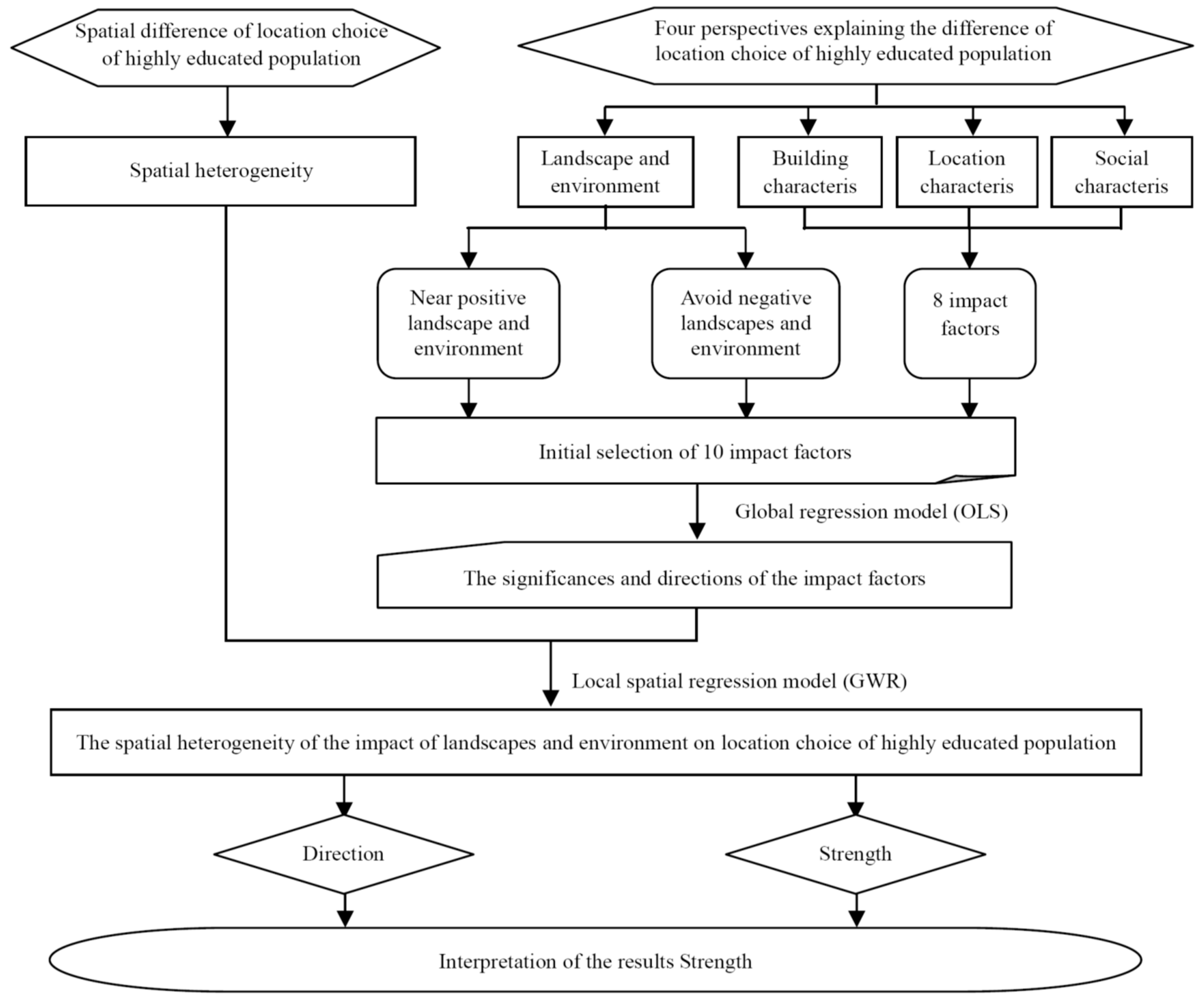
2.2. Conceptual Framework of Livability-Oriented Landscape and Environment

The concept of landscape and environment includes multiple aspects and varies according to different research backgrounds. Based on the understanding of residential location choice, this study proposes a conceptual framework of livability-oriented landscape and environment. This conceptual framework has two basic perspectives: (1) to be near positive landscape and environment, and (2) to avoid negative landscape and environment. We selected three indicators, namely parks, waterfronts, and famous landmarks, to evaluate positive landscape and environment, and selected three other indicators, namely municipal facilities, factory, and logistics and wholesale center, to evaluate negative landscape and environment (Figure 2).

Elaborations of the two perspectives are as follows:

• Near positive landscape and environment (NPLE): This comprises of parks, waterfronts, and famous landmarks which enhance the landscape and environment. Parks [24,45,46] and rivers or lakes [25,26,47] not only create a pleasurable landscape but also improve the environment (such as purifying the air) and boost the microclimate (such as reducing the urban heat island effect) [48,49,50]. As places of daily leisure, these elements have a significant impact on residents’ choice of location [21]. A famous landmark is the symbol of a city and may take the form of important landmark buildings, areas, and scenic spots; for example, Beijing’s Tiananmen Square, Oriental Pearl Tower in Shanghai, West Lake in Hangzhou, and Pearl River New Town in Guangzhou. As important landscape sites and symbols of urban centers, landmarks have aesthetic and landscape values [27], and their surrounding areas often have a well-built environment and a refined urban atmosphere, making them a large attraction for residents [28]. In theory, a highly educated population is more inclined to live in areas close to a positive landscape and environment.
• Avoid negative landscape and environment (ANLE): This comprises municipal facilities, factories, and logistics and wholesale centers, which are likely to exert a negative impact on the landscape and environment [51]. Municipal facilities include airports, train stations, coach stations, highways (or elevated roads), railways, gas stations, funeral homes, substations, sewage treatment plants, garbage disposal sites, signal transmission towers, high-voltage corridors, and more. Municipal facilities constitute negative urban landscape regarding visual and psychological aspects. Pollution is observed in noise, radiation, air quality, odor, hygiene, and safety risks. Some case studies have demonstrated the negative impact of these facilities on housing choices (or housing prices) [22,23,29,31,32]. A factory may also have negative impacts on the surroundings, such as noise and air pollution, so the industrial built environment leads to negative landscape features [33,34]. Further, logistics centers and professional wholesale markets tend to gather many freight vehicles around them, which can cause traffic congestion and generate noise and air pollution. Moreovre, the large and complex flow of people in logistics centers and specialized wholesale markets is likely to have a negative impact on urban safety [34]. In theory, the highly educated population often chooses to live away from negative and closer to positive landscapes and environments.

2.3. Research Design

This study designed a conceptual framework to understand specific areas where landscape and environment have a significant impact on the choice of housing location of the highly educated population, to study the spatial heterogeneity of landscape and environment and the direction and intensity thereof. The analysis process is as follows. First, using data from 1364 communities in the Guangzhou Metropolitan Area, a model of the residential location of highly educated population is built from the perspective of the landscape and environmental characteristics, building characteristics, location characteristics, and social characteristics. Second, we used the ordinary least squares (OLS) model to study the global influencing factors and directions that explain the choice of residential location of Guangzhou’s highly educated population. Third, we used the geographically weighted regression (GWR) model to analyze the spatial heterogeneity of the effects of landscape and environment on the location choice of the highly educated population. Specifically, these include the significant-, direction-, and intensity differences in the influence of landscape and environment on the choice of residential location in different regions. Finally, the results are explained (Figure 3).

The segment of the population that has a bachelor’s degree or above is defined as the highly educated population. The proportionate percentage (%) of the highly educated population among those aged six and above is used to represent the residential attractiveness of the community to the highly educated demographic group. The higher the percentage, the higher the chances of the highly educated population tending to live in the community; this serves as the dependent variable in this study. The two constituent elements of landscape and environment, which have been explained in the co conceptual framework, are the explanatory variables for the residential location of the highly educated population. Further, “building characteristics”, “location characteristics”, and “social characteristics” are the controlling factors, and are composed of a series of indicators as follows:

• Building characteristics: Building age (BAGE), building area per household (BAREA), and housing facilities (HF) were chosen as the three factors reflecting “building characteristics [52,53,54,55,56]”. The highly educated population with a higher income is more inclined to live in housing with a newer building, larger building area, and more complete housing facilities.
• Location characteristic: Location is an important factor to consider when choosing a residential location [57]. It is found here from the three perspectives of daily life convenience (DLC), public services accessibility (PSA), and CBD accessibility. Among them, DLC is jointly evaluated by subway transport-, business service-, and office accessibility. PSA consists of basic education-, medical services-, and cultural and physical activity accessibility. Empirical studies have proved the positive impact of these indicators on housing prices from the perspective of characteristic prices [58,59,60], as they are important factors in choosing residential locations [61,62,63,64,65].
• Social characteristics: Population density (POPD) and employment rate (ER) are two main factors reflecting “social characteristics.” POPD demonstrates the degree of residential congestion in the community. ER is an important indicator of community security and attraction. Higher unemployment will lead to higher crime rates [66]. Theoretically, the choice of residential location of a highly educated population is influenced by POPD and ER.

The detailed definitions, as well as evaluation standards or calculation methods of the above factors, are shown in

Table 1. Definition and evaluation of the variables.

Variables (Symbol)	Definition	Evaluation Standard (Score) or Calculation Method
Dependent variable	Proportion of highly educated population (PHEP)	Proportion of highly educated population among those aged six years and above expressed as a percentage (%)
Explanatory Variables—Landscape and Environment
Near positive landscape and environment (NPLE)	Park accessibility	Within 200 m of parks: (9)
		200–400 m of parks: (7)
		400–800 m of parks: (3)
		Beyond 800 m of parks: (1)
	Waterfront accessibility	Within 200 m of a river (lake): (9)
		200–400 m of river (lake): (7)
		400–800 m of river (lake): (3)
		Beyond 800 m of river (lake): (1)
	Famous landmark accessibility	Within 500 m of famous landmarks: (9)
		500–1000 m of famous landmarks: (5)
		Beyond 1000 m of famous landmarks: (1)
Avoid negative landscape and environment (ANLE)	Avoid municipal facilities	Railway station (500 m), coach station (500 m), highway or elevated road (200 m), railway (80 m), gas station (80 m), funeral home (1000 m), substation (500 m), sewage treatment plant (2000 m), garbage disposal field (4000 m). The base score is 9 and is reduced by 1 for each aversive facility that the community is located near, based on the metrics defined here.
	Avoid factories	Positive standard deviation value examination of the kernel density distribution of factory divided into five grades: community located at 3 sd (1), 2–3 sd (3), 1–2 sd (5), mean to 1 sd (7), and outside the mean (9)
	Avoid logistics and wholesale centers	Positive standard deviation value examination of the kernel density distribution of logistics and wholesale center divided into five grades: Community located at 3 sd (1), 2–3 sd (3), 1–2 sd (5), meanto 1 sd (7), and outside the mean (9)
Control Variables—Building Characteristics
Building age (BAGE)	Community score of average building age	Before 1949 (1), 1949 to 1959 (2), 1960 to 1969 (3), 1970 to 1979 (4), 1980 to 1989 (5), 1990 to 1999 (7), and after 2000 (9). The proportion of each type of household in the community is calculated and multiplied by the corresponding score before adding up (the same calculation method is used for the following building characteristics indicator, BAREA)
Building area per household (BAREA)	Community score of average building area per household	Lower than 10 m2 (1), 10–20 m2 (2), 20–50 m2 (3), 50–80 m2 (4), 80–110 m2 (6), 110–140 m2 (7), 140–200 m2 (8), and over 200 m2 (9)
Housing facilities (HF)	Cooking fuel	No gas (electricity, coal, firewood, other) (1), gas (9)
	Pipe water	No tap water (1), tap water available (9)
	Kitchen	No kitchen (1), shared kitchen with other households (5), independent kitchen (9)
	Bathroom	Shared use of other forms of toilet (1), independent use of other forms of toilet (3), shared use of toilet (5), independent use of toilet (9)
	Bathing facilities	No bathing facilities (1), other forms of bathing facilities (5), uniform hot water supply or home-installed water heaters (9)
Control Variables—Location Characteristics
Daily life convenience (DLC)	Subway accessibility	Within 200 m of subway stations (9), 200–400 m of subway stations (7), 400–800 m of subway stations (5), 800–1500 m of subway stations (3), and beyond 1500 m of subway stations (1)
	Business services accessibility	Positive standard deviation value examination of the Kernel density distribution of business service facility (supermarkets, convenience stores, shopping malls, respectively) divided into five grades: Neighborhood located at 3 sd (9), 2–3 sd (7), 1–2 sd (5), mean to 1 sd (3), outside the mean (1)
	Office accessibility	Positive standard deviation value examination of the Kernel density distribution of office building (office buildings, government agencies, institutions, respectively) divided into 5 grades: Neighborhood located at 3 sd (9), 2–3 sd (7), 1–2 sd (5), mean to 1 sd (3), and outside the mean (1)
Public services accessibility (PSA)	Basic education accessibility	Within the community: provincial key elementary school (9), municipal key elementary school (7); others without provincial key elementary schools or municipal key elementary schools: within 500 m (5) from provincial and municipal key elementary schools (5), within 500 m from ordinary elementary schools (3), 500 m away from all primary schools (1)
	Medical services accessibility	Within 2000 m from third-class hospitals (9), over 2000 m away from third-class hospitals and within 2000 m from general hospitals (5), over 2000 m away from third-class hospitals and general hospitals (1)
	Cultural and physical activities accessibility	Total number of cultural centers, libraries, museums, youth activity centers, science and technology centers, and major stadiums within 1000 m of the community: ≥25 (9), 20–24 (8), 15–19 (7), 10–14 (6), 8–9 (5), 6–7 (4), 4–5 (3), 2–3 (2), 0–1 (1)
CBD accessibility (CBDA)	Distance from CBD	Straight-line distance to the CBD (IFC building); normalize the data to 1–9 points; the closer to the CBD, the higher the score
Control Variables—Social Characteristics
Population density (POPD)	Population density	Population per square kilometer of construction land (%)
Employment rate (ER)	Employment rate	Proportion of employed population to economically active population (%)

. For composite variables (for instance, NPLE, ANLE, HF, DLC, PSA), the factor analysis is used to calculate the weight of indicators. Scores of the variables mentioned above are calculated by weighted summation.

2.4. Data and Data Sources

Data for the PHEP, building characteristics (BAGE, BAREA, and HF), and social characteristics (POPD and ER) are collected from the sixth population census of Guangzhou municipality. NPLE data (Park, Waterfront, and Famous landmark) are derived from “Outline of the Guangzhou Urban Master Plan (2011–2020)” and are obtained by draft vectorization. ANLE and location characteristics (DLC, PSA, and CBDA) data are derived from the 2012 points of interest (POI) database in Guangzhou.

2.5. Methods

2.5.1. Global Regression Analysis

A global regression model was used to find the global factors of differences in the residential locations of Guangzhou’s highly educated population. This was done to verify whether the aforementioned selected factor indicators were reasonable and to examine whether they had an accurate impact on the choice of residential locations of highly educated population. For the study of factors affecting regional differences, the ordinary least squares (OLS) methods are commonly used. We use the OLS model to study the global influencing factors and influence directions that explain the choice of residential location of Guangzhou’s highly educated population.

OLS is a linear model used to study the linear relationship between dependent and independent variables. It is based on the assumption that variables are independent of each other and ignores their spatial information. The OLS model can be expressed as:

$$y_s={\displaystyle \sum _{i=1}^n{\beta }_i{x}_{si}}+{\beta }_0+{\epsilon }_s,\left[{\epsilon }_s~N(0,{\delta }^2)\right]$$

(1)

where, s = 1,…,1364 refers to the Guangzhou communities; y_s denotes the PHEP in the sth community; x_si (i = 1,…,10) represents the variables of the influencing factors, namely NPLE, ANLE, BAGE, BAREA, HF, DLC, PSA, CBDA, POPD, and ER; β_i denotes the regression coefficient of the ith variable; β₀ is a constant term; and ε is the error of the model. The data of dependent and independent variables in this paper are processed in the form of logarithmic standardization.

2.5.2. Geographically Weighted Regression

A global multiple regression model requires only one equation for all data [67] and assumes that this statistical relationship remains consistent everywhere. This kind of statistical relationship will change locally, with different spatial locations. The GWR model allows for local spatial changes in the relationship between independent and dependent variables throughout the space [68,69]. The GWR model we use is similar to OLS, but the OLS method is extended by embedding observed geographic locations into the model. Each parameter is estimated in space, and the parameters change by spatial location [70], which greatly improves the fit of the model. The GWR model can be expressed as:

$$y_s={\displaystyle \sum _{i=1}^n{\beta }_i(u_s,v_s)x_{si}}+{\beta }_0+(u_s,v_s)+{\epsilon }_s,\left[{\epsilon }_s~N(0,{\delta }^2)\right]$$

(2)

where (u_s, v_s) is the geographic location coordinate of community s. Consequently, β₀ (u_s, v_s) is a constant term of the regression model of the community s, with β_i (u_s, v_s) being the local regression coefficient of the ith variable in community s, which varies with the location, and ε is the error term. Each local β_i (u_s, v_s) is used to estimate its neighboring space observations.

The weighted least squares method is used to estimate the elastic coefficient at any point (u_s, v_s) in the study area. The estimated value is expressed as follows:

$$\stackrel{\wedge }{\beta }(u_s,v_s)={\left(X^{T}W(u_s,v_s)X\right)}^{-1}{X}^{T}W(u_s,v_s)y_s$$

(3)

where X is the independent variable matrix and T is the matrix transpose operation. W (u_s, v_s) represents a spatial weight matrix, which is composed of the monotonically decreasing function value of the geographical distance between point s and its surrounding observation points. The points closer to the regression coordinates play a greater role in parameter estimation and may take different functions/forms.

We use the Gauss kernel function to calculate the weights between communities.

$$W_{sk}=\exp \left[-{(d_{sk}/b)}^2\right]$$

(4)

where W_sk represents the Euclidean distance between the position of community s and community k, and b is the optimal bandwidth. W_sk is a continuous monotone decreasing function of d_sk., such that when d_sk = 0, W_sk = 1.

Due to the uneven distribution under observation, communities in Guangzhou’s old- and core- areas are smaller and denser than those in suburban areas. Therefore, where the community is sparsely distributed, the bandwidth distance will become larger, while in the densely distributed communities, the bandwidth distance will become smaller. To obtain the best bandwidth, we use the adjusted value of the Akaike information criterion (AIC_C) [71]. AIC_C is expressed as follows:

$${AIC}_C=2m\ln \hat{\sigma }+m\ln (2\pi )+\frac{m+tr\left(S\right)}{m-2-tr{\left(S\right)}^{\prime }}$$

(5)

where σ is the maximum likelihood estimate of the variance of the random error, and tr(S) denotes the trace of the S matrix.

3. Results and Discussions

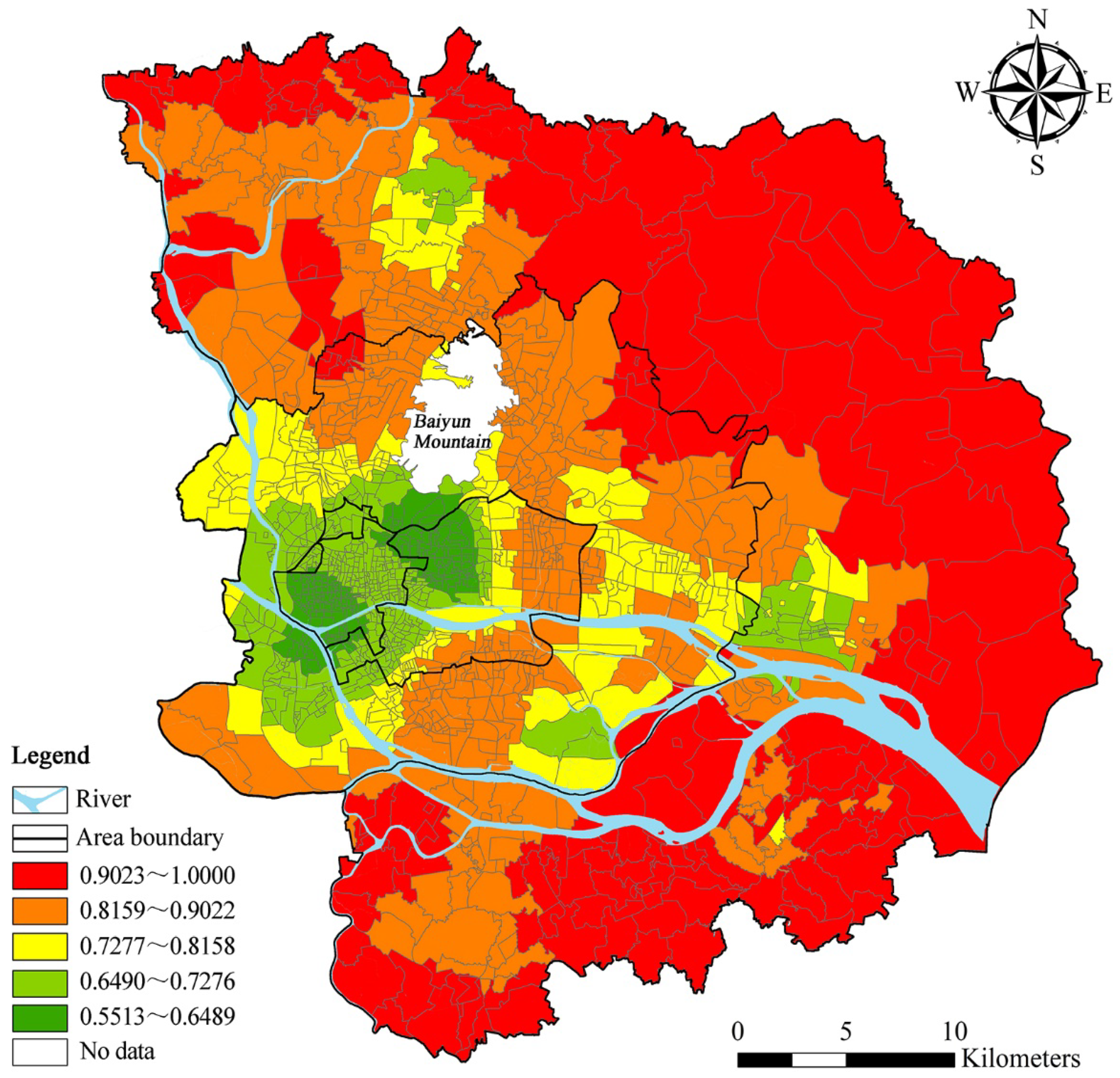
3.1. Spatial Heterogeneity in the Residential Location Choice of Highly Educated Population

Descriptive cluster statistics of the PHEP are shown in Figure 4. A natural breaks (Jenks) method is used as the division thresholds corresponding to five numerical ranges, i.e., 0–7.81%, 7.81–18.10%, 18.10–30.77%, 30.77–51.93%, and 51.93–91.99%, the corresponding number of communities are 655, 409, 201, 76, and 23, respectively. Figure 5 shows the spatial heterogeneity of Guangzhou’s highly educated population drawn by ArcGIS 10.0. Areas with a PHEP higher than 18.10% are mainly distributed in the core area, the northeast fan-shaped region of the urban district, and the “university city” in the suburbs. Among these, the area with a PHEP exceeding 51.93% is where the universities are located. In general, the core area has the highest PHEP, nearly 22.62%, while the PHEP in urban districts is 12.94%, and that in the suburbs is 10.83%. The old area has the lowest PHEP at just 9.84%.

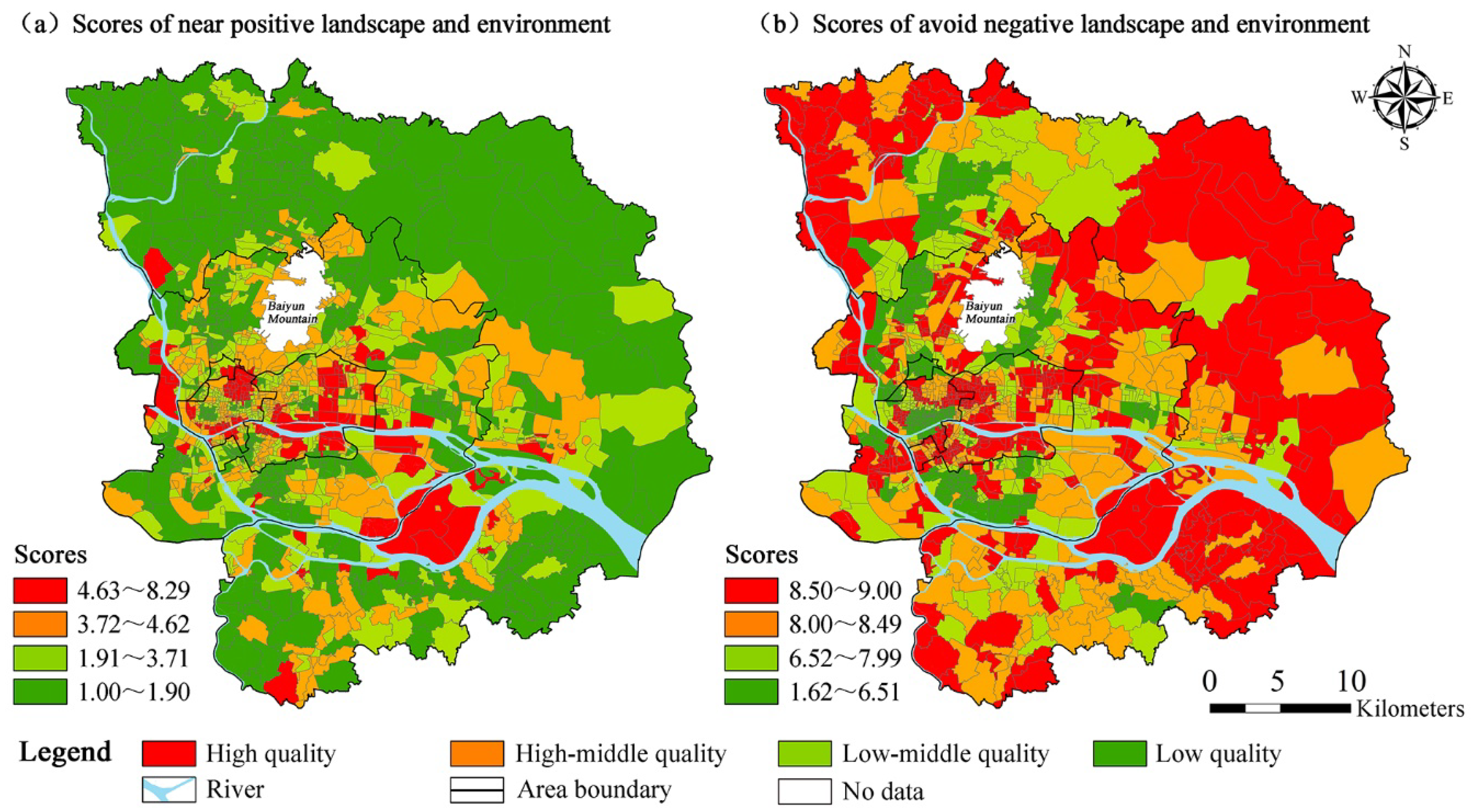
3.2. Spatial Heterogeneity of Landscape and Environment

Using ArcGIS 10.0, a quantile method is used to divide NPLE and ANLE into four grades, ranging from high to low, respectively. A higher score indicates a better landscape and environment. Regarding NPLE, the Pearl River, the new central axis of the core area, and the university city of the suburban areas achieve a higher score. In contrast, regarding ANLE, the core area generally scores higher, indicating that the area is less affected by negative landscape and environment. Several low-scoring communities exist in other areas. Overall, there are differences in the spatial distribution patterns of NPLE and ANLE (Figure 6).

3.3. The Effects of Landscape and Environment on the Residential Location Choice of Highly Educated Population Using the Global Regression Model

It is necessary to analyze how landscape and environment affect the overall situation and the extent of their influence on the choice of residential locations of the highly educated population. Currently, regression analysis is the most widely used method in the field of residential location choice. Among global regression methods, the OLS method is most commonly used to estimate the significance and direction of the independent variable’s influence on the dependent variable. We use GWR4.0 software to run the OLS model. A collinearity test shows that there is no collinearity among the ten factors. The R² and AIC value of OLS are found to be 0.5755 and 3307.51, respectively. OLS regression results show that eight of the ten factors discussed in this study have a significant (0.05 significance level) positive relationship with PHEP, consistent with theoretical expectations (

Table 2. Estimation results of the OLS.

	Coefficient	Std. Error	t/z-Value	p
Intercept	−9.8672 ***	0.9452	−10.4393	0.0000
NPLE	0.3438 ***	0.0458	7.5084	0.0000
ANLE	0.3341 ***	0.0974	3.4312	0.0006
BAGE	−0.3352 ***	0.1191	−2.8144	0.0050
BAREA	2.0697 ***	0.1160	17.8502	0.0000
HF	1.7585 ***	0.2961	5.9381	0.0000
DLC	0.1057 **	0.0494	2.1407	0.0325
PSA	0.3419 ***	0.0654	5.2308	0.0000
CBDA	1.5141 ***	0.1126	13.4524	0.0000
POPD	0.0858 ***	0.0239	3.5921	0.0003
ER	0.0831	0.1645	0.5052	0.6135
R-squared: 0.5755; AIC: 3307.51

*** and ** represent the 0.01 and 0.05 significance levels, respectively.

). The two landscape and environment factors (NPLE and ANLE) comply with theoretical expectations and are significant (0.01 significance level). For every 1% increase in the NPLE (ANLE) score, the PHEP increases by 0.3438% (0.3341%). This shows that globally, landscape and environment have a significant impact on the highly educated population’s choice of residential location.

Regarding controlling factors, BAREA, HF, DLC, PSA, and CBDA also have a significant positive impact on the residential location choice of the highly educated population, which is consistent with theoretical expectations. In contrast, the effect of ER is not significant. Compared to architectural- and social characteristics, landscape and environment-, and location characteristics are more important factors influencing the choice of residential locations of highly educated population. In exchange for better landscape and environment, the highly educated population is willing to accept older housing and higher population density.

To compare the difference of residential location choice between the population with high education and low education, we analyze factors influencing residential location choices of low educated population (defined as junior high school education and below) using the OLS model. Results show that NPLE and ANLE have a significant (0.01 significance level) negative relationship with PHEP. This shows that the obvious difference in the influence of landscape and environment factors on the residential location choices between the highly educated population and low educated population. For every 1% increase in the NPLE (ANLE) score, the proportion of low educated population decreases by 0.1241% (0.1701%).

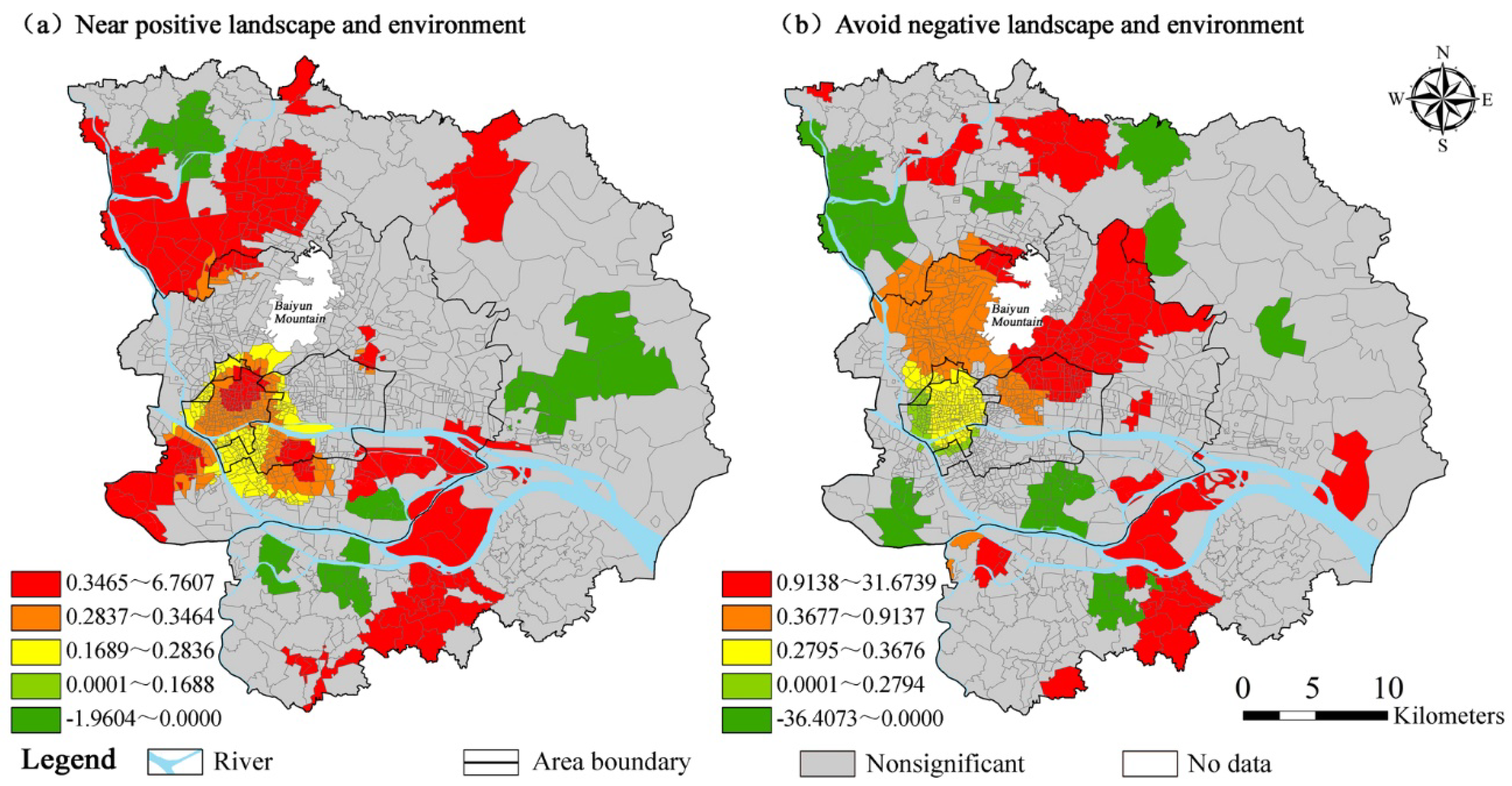
3.4. Impact of the Spatial Heterogeneity of Landscape and Environment on the Residential Location Choice of Highly Educated Population Based on the GWR Model

The spatial distribution of the PHEP in Guangzhou is characterized by heterogeneity. Therefore, it is necessary to further use the GWR model for local spatial regression. The GWR model can account for local spatial changes in the relationship of landscape and environment with Guangzhou’s PHEP throughout the space. It can isolate smaller and relatively homogeneous local areas from the large heterogeneous areas, reducing the impact of spatial heterogeneity. The local regression includes only nearby communities and assigns weights to selected communities based on their respective spatial distance from the target community [71]. We use GWR4.0 software to run the GWR model and choose spherical coordinates as locational variables. The model type is Gaussian. Fixed Gaussian is used to geographic kernel type. The method for optimal bandwidth search is calculated using a golden section search algorithm. The criterion for optimal bandwidth is used to AICc. The best bandwidth calculated is 0.014.

Table 3. Statistics of the local coefficients of GWR.

	Min	Lower Quartile	Median	Upper Quartile	Max	STD
Intercept	−160.5585	−15.3674	−7.7072	−4.0204	336.7557	8.4113
NPLE	−1.9605	0.0458	0.2450	0.3276	6.7607	0.2089
ANLE	−36.4074	0.0323	0.3118	0.7647	31.6739	0.5429
BAGE	−19.2604	−0.9577	−0.3926	−0.0560	10.0277	0.6684
BAREA	−6.1611	1.9259	2.4161	2.9454	7.7807	0.7558
HF	−26.0794	0.5047	1.2780	3.8587	17.1025	2.4862
DLC	−6.1591	−0.0216	0.0868	0.1833	10.8584	0.1519
PSA	−2.8508	−0.1394	0.1279	0.3941	2.9337	0.3955
CBDA	−8.2355	0.4765	1.8765	2.5240	14.5504	1.5178
POPD	−1.6512	−0.0265	0.0020	0.1069	1.8393	0.0989
ER	−51.0185	−1.2040	−0.1115	0.7883	26.0588	1.4769
R-squared: 0.8872; Log likelihood: −739.02; AIC: 2597.86

shows the statistical values of the GWR local coefficients of the model. The GWR’s R², Log-likelihood, and AIC are 0.8872, −739.02, and 2597.86, respectively. These indicate that the model has acceptable overall goodness of fit, and can better explain the relationship between the residential location choice and the determinants taken into consideration by the highly educated population than the global regression model (OLS).

The ten variables are included in the model on the premise that AIC is minimized and non-collinear. AIC and ANOVA analyses (F-test) both showed statistical significance. The spatial distribution map of local R² affecting the PHEP is shown in Figure 7. The local R², ranging from 0.5513 to 1, reflects the comprehensive impact of the ten variables on PHEP. A natural breaks (Jenks) method is used as the division Local R² to five numerical ranges. In general, while the Local R² in the old area and its surrounding areas are relatively low, the suburban area has the highest R² (with R² in most communities exceeding 0.9023). This shows that these factors have a more significant impact on the housing choices of the highly educated population in suburban areas.

A GWR model was established to explore the correlation between PHEP and various factors, and a pseudo-t-test (p < 0.05) was performed to test the statistical significance of the parameters (

Table 4. Statistical significance of the parameters set by GWR models for ten factors.

	p < 0.05	+	−
NPLE	50.81%	47.80%	3.01%
ANLE	48.02%	44.28%	3.74%
BAGE	35.41%	5.65%	29.77%
BAREA	86.44%	84.90%	1.54%
HF	28.01%	27.57%	0.44%
DLC	59.82%	47.87%	11.95%
PSA	21.19%	16.35%	4.84%
CBDA	59.68%	51.83%	7.84%
POPD	49.27%	31.74%	17.52%
ER	55.50%	22.65%	32.84%

). The results reveal a significant positive correlation between NPLE and PHEP in 47.80% of the communities, and a significant positive correlation between ANLE and PHEP in 44.28% of the communities (consistent with theoretical expectations). While these two values are lower than BAREA (84.90%), CBDA (51.83%) and DLC (47.87%), they are higher than POPD (31.74%), HF (27.57%), ER (22.65%), PSA (16.35%), and BAGE (5.65%).

The direction, intensity, and significance of spatial distribution in the correlation of landscape and environment (NPLE and ANLE) with PHEP are shown in Figure 8. A quantile method is used to divide estimated coefficients into five grades. Insignificant areas are represented in gray. Regarding NPLE, the areas where NPLE and PHEP have a significantly positive correlation are mainly distributed in the old area, the southern part of the urban district (near the old area or the core area), and parts of the suburban area. Regarding ANLE, the areas with a significant positive correlation between ANLE and PHEP are distributed in the old area (although the coefficient is relatively low), north of the core area, and north of the urban district (near Baiyun Mountain), showing a decentralized distributive pattern in the suburbs. It can, therefore, observed that there is spatial heterogeneity in the degree of influence of landscape and environment on the highly educated population’s choice of residential location. Communities with a significant positive relationship between landscape and environment and choice of residential location among the highly educated population show a spatially concentrated distribution.

The proportions of communities with significant positive correlations between landscape and environment and PHEP in the four perimeter areas (old area, core area, urban district, and suburban area) were calculated (

Table 5. Geographical distribution differences in the significant positive correlation between landscape and environment and highly educated population.

	Old Area	Core Area	Urban District	Suburban
NPLE	99.58%	55.77%	30.97%	27.04%
ANLE	94.96%	43.91%	37.48%	16.61%

). The proportion of communities with a significant positive correlation between landscape and environment and PHEP was the highest for the old area, with NPLE and ANLE reaching 99.58% and 94.96%, respectively. Suburban areas had the lowest proportion percentage, with NPLE and ANLE achieving only 27.04% and 16.61%, respectively. It can be seen that the influence of landscape and environment on the highly educated population’s choice of residential location is mainly reflected in the old area, and is least perceptible in the suburban area.

3.5. Discussions

The highly educated population often has higher socioeconomic status, and high-quality landscape and environment are scarce resources of the city. Therefore, the mechanisms of the effects of landscape and environment on the residential location choice are as follows: From the perspective of housing affordability, the better the landscape and environment, the higher the “threshold” of purchasing or renting. Through space competition or price competition, the population with higher education is more likely to have the property rights or rental rights of communities with better landscape and environment. From the perspective of the population’s residential choice behavior, when all other housing conditions are the same, people are more inclined to choose the community with a high-quality landscape and environment. However, due to the limited number of such communities, only the population with higher education (with higher socio-economic status) is more likely to occupy them. From the perspective of human needs, the landscape and environment are higher-level living factors beyond the basic living needs. Compared with a low educated population (often only focusing on basic living factors), the highly educated population usually has higher requirements on landscape and environment. It is worth noting that there is significant spatial heterogeneity in the educational background structure of urban population and landscape and environmental conditions and, therefore, the degree of the mechanism is bound to show spatial heterogeneity.

This research constructs a comprehensive system of factors (including positive and negative landscape and environment) for location choice by adopting a livability angle, combining landscape and environment, architectural characteristics, and location characteristics to verify whether landscape and environment exert an impact and spatial heterogeneity of such an impact. The research, based on the global regression model OLS, proves the theoretical hypothesis that landscape and environment have a significant impact on the residential location choice of highly educated population. When choosing a location for their residence, highly educated people prefer positive landscapes and environment (parks, waterfronts, and famous landmarks) and not negative landscape and environment (municipal facilities, factories, logistics centers, and professional wholesale markets). The findings are consistent with previous studies. Further, the empirical analysis based on GWR explores the regional differences in the impact of landscape and environment on the highly educated population’s choice of residential location in more detail than in previous studies (which are based on global studies). It focuses on analyzing the spatial heterogeneity of this impact relationship, ignored in previous studies. The significance of the discovery is that the conclusions of this study will be of reference value to understand the spatial limitations of landscape and environment on the residential location choices of the highly educated population. This provides a reference for the researchers to make the different spatial policies of urban landscape and environment improvement. Based on these findings, the existing research (based on global research) can make further progress from the perspective of spatial differentiation. By observing the relationship between landscape and environment and talent attraction, this study serves as a reference point for policymaking regarding the construction of livable and innovative cities. It offers theoretical support for sustainable urban development.

4. Conclusions and Policy Implications

4.1. Conclusions

This study establishes a research framework for the highly educated population’s choice of residential locations based on urban landscape and environment. It sets up a dataset of the PHEP and its influencing factors in 1364 communities in Guangzhou. GWR technology is used to analyze the spatial heterogeneity in the direction and degree of the influence of landscape and environment on the highly educated population’s residential location choices. The research conclusions are summarized as follows.

Studies show a high degree of spatial heterogeneity in the distribution of the highly educated population in Guangzhou. Generally, the core area has the highest PHEP, while the old area has the lowest. Overall, the landscape and environment in the core areas are of the highest quality. However, the spatial patterns of NPLE and ANLE are not the same in Guangzhou.

A global regression model (OLS) was used to verify the relationship between the two aspects of landscape and environment (NPLE and ANLE) and the distribution of the highly educated population, and the significance thereof. The results show that NPLE and ANLE have a significant impact on the choice of residential location of the highly educated population, and the direction of influence is consistent with theoretical expectations. For every 1% increase in the NPLE (ANLE) score, the PHEP increases by 0.3438% (0.3341%).

The spatial heterogeneity of the relationship between landscape and environment and the PHEP was analyzed using the GWR method. Results show that GWR has better model performance than OLS, with larger R² and lower AIC. The effects of both NPLE and ANLE on PHEP show spatial heterogeneity. NPLE and ANLE have a positive and significant impact on the choice of residential location for the highly educated population in 47.80% and 44.28% of the communities, respectively. The areas with considerable influences show spatial clustering in distribution and are mainly located in the old area. In the suburban area, such an influence is weaker.

4.2. Policy Implications

The conclusions of this study highlight the importance of landscape and environment in attracting highly educated people. Moreover, the impact of landscape and environment on highly educated people varies according to spatial location. Therefore, in the formulation of policies and action plans for urban landscape shaping and environmental improvement, attention should be paid to spatial differences within cities. It is recommended that a spatially differentiated policy be adopted, and urban renewal and environment improvement plans are implemented in a differentiated manner as follows.

First, improve the urban restoration of the old area and the landscape environment thereof. The results of this study indicate that landscape and environment have the most significant impact on the highly educated population’s choice of residential location in the old area; meanwhile, the old area hosts the lowest PHEP. Therefore, enhancing the landscape and environment of the old area will attract highly educated people. Suggested measures to improve the landscape and environment are as follows:

• As the old area is densely built, resulting in a poorly built environment, it is recommended that more public space be made available therein by making full use of the land area for increasing green space.
• The old area has a higher concentration of specialized wholesale markets, causing traffic congestion and noise pollution. These markets should be relocated to places with convenient transportation in the suburbs. In their place, urban green spaces, squares, creative industrial parks, science and technology parks, cultural exhibition venues, or urban public event venues should be built to enhance the landscape of the old area and improve environmental conditions.
• It is recommended that more efforts be made to renovate municipal infrastructure in the old area to reduce the negative impact of the polluting municipal facilities on the environment of the old area.

Second, reinforce the construction of high-quality landscape and environment facilities in the suburb. The results of this study show that the quality of the suburban landscapes and the environment has the lowest score, and the PHEP in the suburb is exceedingly low. Therefore, it is necessary to reserve more space for the construction of suburban parks, public event venues, cultural event facilities, and landmark buildings. Thus, the accessibility of high-quality landscape and environment elements could be improved, and the residential attractiveness of the suburb to the highly educated population would also increase, relieving the pressure and living costs in the core area. Additionally, it is necessary to re-arrange polluting municipal and transportation facilities, keeping them farther from residential areas to reduce their impact on the landscape and environment of the residential areas.

Third, the quality of the existing landscape and environmental facilities should be further improved for the core area and urban district. They should be developed into livable areas through high-level planning and construction aimed at creating a world-class environment to attract global talent.

4.3. Limitations and Future Research

We use classical GWR to study the spatial heterogeneity of influencing factors. However, all factors may not have the effect of heterogeneity in space, and some of them having small changes in space can be ignored, such as the building area. The influence intensity of these factors may be consistent throughout the study; that is, not all variables can be estimated in the same way in GWR. Considering this limitation of GWR, in the next research, we will introduce the mixed GWR model to analyze the spatial heterogeneity of specific influencing factors, to get precise results.

From the perspective of the selection of influencing factors, ten factors (composed of 22 indicators) are considered in this study. However, theoretically, several factors can affect the residential choice of highly educated people. This paper does not cover all the factors because of data acquisition limitations. In future studies, the number of variables can be further increased to improve the model fit.

References

1. Knox, P.; Pinch, S. Urban Social Geography: An Introduction; Routledge: London, UK, 2014. [Google Scholar]
2. De Vos, J.; Alemi, F. Are young adults car-loving urbanites? Comparing young and older adults’ residential location choice, travel behavior and attitudes. Transp. Res. Part A-Policy Pract. 2020, 132, 986–998. [Google Scholar] [CrossRef]
3. Beckers, P.; Boschman, S. Residential choices of foreign highly skilled workers in the Netherlands and the role of neighbourhood and urban regional characteristics. Urban Stud. 2019, 56, 760–777. [Google Scholar] [CrossRef] [Green Version]
4. Wen, H.; Zhao, Z. Talent introduction and housing price: A tale of Xi’an. Appl. Econ. Lett. 2019, 26, 954–962. [Google Scholar] [CrossRef]
5. Cho, E.J.; Rodriguez, D.A.; Song, Y. The Role of Employment Subcenters in Residential Location Decisions. J. Transp. Land Use 2008, 1, 121–151. [Google Scholar]
6. Vega, A.; Reynolds-Feighan, A. A methodological framework for the study of residential location and travel-to-work mode choice under central and suburban employment destination patterns. Transportation Transp. Res. Part a-Policy Pract 2009, 43, 401–419. [Google Scholar] [CrossRef] [Green Version]
7. Chu, Y.-L.; Deng, Y.; Liu, R. Impacts of New Light Rail Transit Service on Riders’ Residential Relocation Decisions. J. Public Transp. 2017, 20, 152–165. [Google Scholar] [CrossRef] [Green Version]
8. Lasley, P. Influence of Transportation on Residential Choice: A Survey of Texas REALTORS® on Factors Affecting Housing Location Choice. Ph.D. Thesis, Texas A & M University, College Station, TX, USA, 2017. [Google Scholar]
9. Epple, D.; Filimon, R.; Romer, T. Equilibrium among local jurisdictions: Toward an integrated treatment of voting and residential choice. J. Public Econ. 1984, 24, 281–308. [Google Scholar] [CrossRef]
10. Geyer, J. Housing demand and neighborhood choice with housing vouchers. J. Urban Econ. 2017, 99, 48–61. [Google Scholar] [CrossRef]
11. Rosen, E. Horizontal Immobility: How Narratives of Neighborhood Violence Shape Housing Decisions. Am. Sociol. Rev. 2017, 82, 270–296. [Google Scholar] [CrossRef]
12. Bhat, C.R.; Guo, J.Y. A comprehensive analysis of built environment characteristics on household residential choice and auto ownership levels. Transp. Res. Part B-Methodol. 2007, 41, 506–526. [Google Scholar] [CrossRef] [Green Version]
13. Liao, F.H.; Farber, S.; Ewing, R. Compact development and preference heterogeneity in residential location choice behaviour: A latent class analysis. Urban Stud. 2015, 52, 314–337. [Google Scholar] [CrossRef]
14. Ettema, D.; Nieuwenhuis, R. Residential self-selection and travel behaviour: What are the effects of attitudes, reasons for location choice and the built environment? J. Transp. Geogr. 2017, 59, 146–155. [Google Scholar] [CrossRef]
15. Kroesen, M. Residential self-selection and the reverse causation hypothesis: Assessing the endogeneity of stated reasons for residential choice. Travel Behav. Soc. 2019, 16, 108–117. [Google Scholar] [CrossRef]
16. Wolpert, J. Behavioral aspects of the decision to migrate. Papers Reg. Sci. Assoc. 1965, 15, 159–169. [Google Scholar] [CrossRef]
17. Setyowati, N.D.A. The Impact of Waterfront Redevelopment on Housing Values: The Case of Canalside Buffalo Waterfront. Ph.D. Thesis, State University of New York at Buffalo, Buffalo, NY, USA, 2017. [Google Scholar]
18. Lotfi, S.; Despres, C.; Lord, S. Are sustainable residential choice also desirable? A study of household satisfaction and aspirations with regard to current and future residential location. J. Hous. Built Environ. 2019, 34, 283–311. [Google Scholar] [CrossRef]
19. Yin, L.; Muller, B. Residential location and the biophysical environment: Excurban development agents in a heterogeneous landscape. Environ. Plan. B-Plan. Design 2007, 34, 279–295. [Google Scholar] [CrossRef]
20. Źróbek, S.; Trojanek, M.; Źróbek-Sokolnik, A.; Trojanek, R. The influence of environmental factors on property buyers’ choice of residential location in Poland. J. Int. Stud. 2015, 7, 163–173. [Google Scholar]
21. Tu, G.; Abildtrup, J.; Garcia, S. Preferences for urban green spaces and peri-urban forests: An analysis of stated residential choices. Landsc. Urban Plan. 2016, 148, 120–131. [Google Scholar] [CrossRef] [Green Version]
22. Brasington, D.M.; Hite, D. Demand for environmental quality: A spatial hedonic analysis. Reg. Sci. Urban Econ. 2005, 35, 57–82. [Google Scholar] [CrossRef] [Green Version]
23. Gurran, N.; Phibbs, P. When Tourists Move In: How Should Urban Planners Respond to Airbnb? J. Am. Plan. Assoc. 2017, 83, 80–92. [Google Scholar] [CrossRef] [Green Version]
24. Czembrowski, P.; Kronenberg, J. Hedonic pricing and different urban green space types and sizes: Insights into the discussion on valuing ecosystem services. Landsc. Urban Plan. 2016, 146, 11–19. [Google Scholar] [CrossRef]
25. Bin, O.; Czajkowski, J.; Li, J.; Villarini, G. Housing Market Fluctuations and the Implicit Price of Water Quality: Empirical Evidence from a South Florida Housing Market. Environ. Resour. Econ. 2017, 68, 319–341. [Google Scholar] [CrossRef]
26. Kim, H.N.; Boxall, P.C.; Adamowicz, W.L. Analysis of the economic impact of water management policy on residential prices: Modifying choice set formation in a discrete house choice analysis. J. Choice Model. 2019, 33, 100148. [Google Scholar] [CrossRef]
27. Been, V.; Ellen, I.G.; Gedal, M.; Glaeser, E.; McCabe, B.J. Preserving history or restricting development? The heterogeneous effects of historic districts on local housing markets in New York City. J. Urban Econ. 2016, 92, 16–30. [Google Scholar] [CrossRef]
28. Wen, H.; Chu, L. Temporal and Spatial Effects of Urban Center on Housing Price—A Case Study on Hangzhou, China. World J. Soc. Sci. Res. 2018, 5, 89–97. [Google Scholar]
29. Diao, M.; Qin, Y.; Sing, T.F. Negative Externalities of Rail Noise and Housing Values: Evidence from the Cessation of Railway Operations in Singapore. Real Estate Econ. 2016, 44, 878–917. [Google Scholar] [CrossRef]
30. Yassin, A.M.; Diah ML, M.; Safian EE, M. Determining the Impact of Aircraft Noise towards Residential Property Price. In MATEC Web of Conferences; EDP Sciences: Jules, France, 2019; Volume 266, p. 02005. [Google Scholar]
31. Nelson, A.C.; Genereux, J.; Genereux, M. Price effects of landfills on house values. Land Econ. 1992, 68, 359–365. [Google Scholar] [CrossRef]
32. Banfi, S.; Filippini, M.; Horehájová, A. Valuation of Environmental Goods in Profit and Non-Profit Housing Sectors: Evidence from the Rental Market in the City of Zurich. Swiss J. Econ. Stat. 2008, 144, 631–654. [Google Scholar] [CrossRef] [Green Version]
33. Li, M.M.; Brown, H.J. Micro-neighborhood externalities and hedonic housing prices. Land Econ. 1980, 56, 125–141. [Google Scholar] [CrossRef]
34. Wang, Y.; Zhao, L.; Sobkowiak, L.; Guan, X.; Wang, S. Impact of urban landscape and environmental externalities on spatial differentiation of housing prices in Yangzhou City. J. Geogr. Sci. 2015, 25, 1122–1136. [Google Scholar] [CrossRef] [Green Version]
35. Frenkel, A.; Bendit, E.; Kaplan, S. The linkage between the lifestyle of knowledge-workers and their intra-metropolitan residential choice: A clustering approach based on self-organizing maps. Comput. Environ. Urban Syst. 2013, 39, 151–161. [Google Scholar] [CrossRef] [Green Version]
36. Millsap, A. Location choice in early adulthood: Millennials versus Baby Boomers. Papers Reg. Sci. 2018, 97, S139–S167. [Google Scholar] [CrossRef]
37. Shilling, C. Social Space, Gender Inequalities and Educational Differentiation. Br. J. Sociol. Educ. 1991, 12, 23–44. [Google Scholar] [CrossRef]
38. Wu, Q.; Edensor, T.; Cheng, J. Beyond Space: Spatial (Re)Production and Middle-Class Remaking Driven by Jiaoyufication in Nanjing City, China. Int. J. Urban Reg. Res. 2018, 42, 1–19. [Google Scholar] [CrossRef]
39. Li, S.; Lyu, D.; Huang, G.; Zhang, X.; Gao, F.; Chen, Y.; Liu, X. Spatially varying impacts of built environment factors on rail transit ridership at station level: A case study in Guangzhou, China. J. Transp. Geogr. 2020, 82, 102631. [Google Scholar] [CrossRef]
40. Zhou, S.; Deng, L.; Kwan, M.-P.; Yan, R. Social and spatial differentiation of high and low income groups’ out-of-home activities in Guangzhou, China. Cities 2015, 45, 81–90. [Google Scholar] [CrossRef]
41. Han, Y.; Wu, X. Language policy, linguistic landscape and residents’ perception in Guangzhou, China: Dissents and conflicts. Curr. Issues Lang. Plan. 2019, 1–25. [Google Scholar] [CrossRef]
42. Suda, K. A Room of One’s Own: Highly Educated Migrants’ Strategies for Creating a Home in Guangzhou. Popul. Space Place 2016, 22, 146–157. [Google Scholar] [CrossRef]
43. Zhao, P.; Kwan, M.-P.; Zhou, S. The Uncertain Geographic Context Problem in the Analysis of the Relationships between Obesity and the Built Environment in Guangzhou. Int. J. Environ. Res. Public Health 2018, 15, 308. [Google Scholar] [CrossRef] [Green Version]
44. Chen, T.; Lang, W.; Li, X. Exploring the Impact of Urban Green Space on Residents’ Health in Guangzhou, China. J. Urban Plan. Dev. 2020, 146, 05019022. [Google Scholar] [CrossRef]
45. Espey, M.; Owusu-Edusei, K. Neighborhood Parks and Residential Property Values in Greenville, South Carolina. J. Agric. Appl. Econ. 2001, 33, 487–492. [Google Scholar] [CrossRef] [Green Version]
46. Stenger, A.; Harou, P.; Navrud, S. Valuing environmental goods and services derived from the forests. J. For. Econ. 2009, 15, 1–14. [Google Scholar] [CrossRef]
47. Luttik, J. The value of trees, water and open space as reflected by house prices in the Netherlands. Landsc. Urban Plan. 2000, 48, 161–167. [Google Scholar] [CrossRef]
48. Chen, X.; Su, Y.; Li, D.; Huang, G.; Chen, W.; Chen, S. Study on the cooling effects of urban parks on surrounding environments using Landsat TM data: A case study in Guangzhou, southern China. Int. J. Remote Sens. 2012, 33, 5889–5914. [Google Scholar] [CrossRef]
49. Wen, H.; Xiao, Y.; Zhang, L. Spatial effect of river landscape on housing price: An empirical study on the Grand Canal in Hangzhou, China. Habitat Int. 2017, 63, 34–44. [Google Scholar] [CrossRef]
50. Cheung, P.K.; Jim, C.Y. Differential cooling effects of landscape parameters in humid-subtropical urban parks. Landsc. Urban Plan. 2019, 192, 103651. [Google Scholar] [CrossRef]
51. Li, R.Y.M.; Chau, K.W.; Li, M.H.; Leung, T.H. Negative environmental externalities and housing price: A Hedonic model approach. In Econometric Analyses of International Housing Markets; Routledge: London, UK, 2016; pp. 109–123. [Google Scholar]
52. Phe, H.H.; Wakely, P. Status, quality and the other trade-off: Towards a new theory of urban residential location. Urban Stud. 2000, 37, 7–35. [Google Scholar] [CrossRef]
53. Goodman, A.C.; Thibodeau, T.G. Housing market segmentation and hedonic prediction accuracy. J. Hous. Econ. 2003, 12, 181–201. [Google Scholar] [CrossRef] [Green Version]
54. Stevenson, S. New empirical evidence on heteroscedasticity in hedonic housing models. J. Hous. Econ. 2004, 13, 136–153. [Google Scholar] [CrossRef]
55. Leung, K.M.; Yiu, C.Y. Rent determinants of sub-divided units in Hong Kong. J. Hous. Built Environ. 2019, 34, 133–151. [Google Scholar] [CrossRef]
56. Wittowsky, D.; Hoekveld, J.; Welsch, J.; Steier, M. Residential housing prices: Impact of housing characteristics, accessibility and neighbouring apartments—A case study of Dortmund, Germany. Urban, Plan. Transp. Res. 2020, 8, 44–70. [Google Scholar] [CrossRef] [Green Version]
57. Schirmer, P.M.; van Eggermond, M.A.B.; Axhausen, K.W. The role of location in residential location choice models: A review of literature. J. Transp. Land Use 2014, 7, 3–21. [Google Scholar] [CrossRef]
58. Qin, B.; Han, S.S. Emerging Polycentricity in Beijing: Evidence from Housing Price Variations, 2001–2005. Urban Stud. 2013, 50, 2006–2023. [Google Scholar] [CrossRef]
59. Yang, L.; Wang, B.; Zhou, J.; Wang, X. Walking accessibility and property prices. Transp. Res. Part D-Transp. Environ. 2018, 62, 551–562. [Google Scholar] [CrossRef]
60. Cao, K.; Diao, M.; Wu, B. A Big Data-Based Geographically Weighted Regression Model for Public Housing Prices: A Case Study in Singapore. Ann. Am. Assoc. Geogr. 2019, 109, 173–186. [Google Scholar] [CrossRef]
61. Weisbrod, G.; Lerman, S.R.; Ben-Akiva, M. Tradeoffs in residential location decisions: Transportation versus other factors. Transp. Policy Decis. Mak. 1980, 1, 13–26. [Google Scholar]
62. Cervero, R.; Wu, K.L. Polycentrism, commuting, and residential location in the San Francisco Bay Area. Environ. Plan. A 1997, 29, 865–886. [Google Scholar] [CrossRef]
63. Kim, J.H.; Pagliara, F.; Preston, J. The intention to move and residential location choice behaviour. Urban Stud. 2005, 42, 1621–1636. [Google Scholar] [CrossRef]
64. Zondag, B.; Pieters, M. Influence of accessibility on residential location choice. In Transportation and Land Development 2005; Transportation Research Board of the National Academies: Washington, DC, USA, 2005; pp. 63–70. [Google Scholar]
65. Humphreys, J.; Ahern, A. Is travel based residential self-selection a significant influence in modal choice and household location decisions? Transp. Policy 2019, 75, 150–160. [Google Scholar] [CrossRef]
66. Raphael, S.; Winter-Ebmer, R. Identifying the effect of unemployment on crime. J. Law Econ. 2001, 44, 259–283. [Google Scholar] [CrossRef] [Green Version]
67. Wang, Y.; Wang, S.; Li, G.; Zhang, H.; Jin, L.; Su, Y.; Wu, K. Identifying the determinants of housing prices in China using spatial regression and the geographical detector technique. Appl. Geogr. 2017, 79, 26–36. [Google Scholar] [CrossRef]
68. Bitter, C.; Mulligan, G.F.; Dall’erba, S. Incorporating spatial variation in housing attribute prices: A comparison of geographically weighted regression and the spatial expansion method. J. Geogr. Syst. 2007, 9, 7–27. [Google Scholar] [CrossRef] [Green Version]
69. Hanink, D.M.; Cromley, R.G.; Ebenstein, A.Y. Spatial Variation in the Determinants of House Prices and Apartment Rents in China. J. Real Estate Financ. Econ. 2012, 45, 347–363. [Google Scholar] [CrossRef]
70. Brunsdon, C.; Fotheringham, A.S.; Charlton, M.E. Geographically weighted regression: A method for exploring spatial nonstationarity. Geogr. Anal. 1996, 28, 281–298. [Google Scholar] [CrossRef]
71. Mou, Y.; He, Q.; Zhou, B. Detecting the Spatially Non-Stationary Relationships between Housing Price and Its Determinants in China: Guide for Housing Market Sustainability. Sustainability 2017, 9, 1826. [Google Scholar] [CrossRef] [Green Version]
Figure 1. Study area.
Sustainability 12 03869 g001
Figure 2. Conceptual framework of livability-oriented landscape and environment.
Sustainability 12 03869 g002
Figure 3. Research design.
Sustainability 12 03869 g003
Figure 4. Descriptive cluster statistics for PHEP in the communities.
Sustainability 12 03869 g004
Figure 5. The spatial heterogeneity pattern of PHEP in Guangzhou.
Sustainability 12 03869 g005
Figure 6. The spatial heterogeneity pattern of positive and negative landscape and environment with the quantile method in Guangzhou; (a) Scores of near positive landscape and environment; (b) Scores of avoid negative landscape and environment.
Sustainability 12 03869 g006
Figure 7. The spatial pattern of Local R2 factors affecting PHEP based on the GWR model.
Sustainability 12 03869 g007
Figure 8. The spatial pattern of local parameter estimates of positive and negative landscape and environment (NPLE and ANLE) based on the GWR model; (a) Near positive landscape and environment; (b) Avoid negative landscape and environment.
Sustainability 12 03869 g008