Optimization of a Combination of Thermal Insulation and Cool Roof for the Refurbishment of Social Housing in Southern Spain

Abstract

Social housing built in the middle of the last century in Spain suffers from poor thermal insulation conditions that cause situations of discomfort and energy poverty. For this reason, the energetic refurbishment of the envelope of this social building stock is necessary to overcome these situations and reduce energy consumption aimed at achieving interior comfort for its occupants. The goal of this work is to optimize a constructive solution that combines cool roof techniques with the use of thermal insulation applied to the refurbishment of the roof of buildings belonging to a quarter of social housing in Seville, Spain. The optimization analysis is based on the computation of the energy performance of the roofs when the energy retrofitting measure is applied, considering a variety of combinations of solar reflective coatings and insulation layer thickness, performing a dynamic analysis that accounts for the aging effect of the cool coats on the monthly roof energy performance and on the economic balance for the whole life cycle (LC) span. Economic and energy optimization analysis show that a suitable combination of cool roof emissivity and insulation layer thickness produces significant savings in the operational energy and in the economic profitability of the proposed retrofitting measure: the optimum combination obtained provides for the entire life cycle timespan an energy savings of 5.71 GJ/m${}^2$ and a cost savings equivalent to the $63.1\%$ of the total costs when compared to the non-refurbished roof. The application of a time-dependent pattern for the changes on time produced by the aging effect on the cool roof emissivity, and its effects on the optimization of the combination of cool roof and insulation layer, can be considered novel in literature, both from an energy and an economic point of view.

1. Introduction

The building sector is responsible for around $40\%$ of final energy consumption in Europe and is a major source of CO${}_2$ emissions. In order to reduce these emissions, in the last few decades, efforts have been made, consisting largely of the promulgation of regulations for the implementation of energy savings and efficiency measures, such as the Spanish norm DB-HE-2019 [1], which establishes new standards for the reduction of energy consumption in buildings, in accordance with the directives set by the EU for the H2030 [2], which establishes as goals for 2030 an improvement in energy efficiency equal to or greater than $32.5\%$, cuts in greenhouse gas emissions equal to or greater than 40%, and a share for renewable energy equal to or greater than $32\%$, all from 1990 levels [2].

In climates characterized by mild winters and very long hot seasons, such as the case of southern Spain and much of the Mediterranean area, a large amount of energy consumption is necessary to obtain the internal comfort of buildings during the cooling season. This poses a serious problem in the case of the social park housing built in southern Spain in the mid-twentieth century, in which envelopes often lack thermal insulation.

The energy efficiency of roofs has been object of a wide research focused on the enhancement and the optimization of its energy performance. This is largely justified by the fact that the roof is the envelope component that receives the most solar radiation in summer and in winter is responsible of an important percentage of the heat losses. Two widely used types of techniques aim to improve the thermal performance of roofs: those that modify their thermal properties, how to add or change thermal insulation, and those who carry out roof surface treatments, how to install radiant barriers or cool roofs. Taking into account that, in the geographical context considered here, in summer, most of the time, the sky is clear, and, in winter, the temperatures are not too cold, the cool roof technique seems advisable to lower the temperature of the roof, while the combination with a layer of insulation can help to achieve indoor comfort conditions and reduce energy consumption for this purpose.

Yu et al. [3] analyzed the optimum thickness of the thermal insulation installed on the roof of a residential building, and they studied different colors for the outer roof surface; to carry out the analysis, a life-cycle cost analysis (LCCA) was performed by considering solar-air degree-hours and four cities representing different China geographical regions; authors concluded that the effect of the colors on the optimal insulation thickness is different for each city. Gentle et al. [4] studied the energy behavior of a roof, analyzing different combinations of solar albedo, thermal emittance, and thermal resistance of a roof; a cost benefit assessment of the different combinations was performed that concluded the importance of high values for the roof albedo. Ramamurthy et al. [5] used the minimization of yearly costs for heating and cooling in order to determine the optimal combination of roof solar albedo and insulation thickness; they concluded that an albedo greater than 0.7, combined with a polyiso foam insulation of 18 cm, significantly reduces thermal flux through the roof when applied to new constructions; likewise, they found that, if installations costs are included in the analysis, the optimal combination is reached for a 4-inch insulation thickness with a payback period of 13 years. Arumugam et al. [6] studied the combination of solar reflective coating, radiant barriers, and thermal insulation for a roof by using EnergyPlus; a total of five climatic zones in India and 88 different roof combinations were analyzed; through an economic analysis, they found that the use of solar reflective coating and radiant barriers on the roof reduced the need for insulation layer for all the climatic regions analyzed.

Other studies have focused on optimizing the properties of the roof. Piselli et al. [7], by using dynamic energy computation, developed a method to perform an optimization analysis; the objective of this analysis was to optimize the solar reflectivity of the roof surface to minimize yearly energy loads for conditioning the building; the analysis was carried out by considering five cities of Italy located in different climate zones as the case study; from the performed optimization analysis, it was concluded that the the climate context is the most influential factor on the optimum roof solar reflectance.

Shi and Zhang [8] studied the effect on the reduction of annual energy loads of different solar reflectance and long-wave emissivity combinations for the outer surface of the building envelope; the study was carried out in 35 different climatic zones of the world and concluded that the greatest potential for energy savings is obtained for tropical climates and for high solar reflectance and high long-wave emissivity values.

Furthermore, a large number of studies deal with usefulness of cool roofs to improve indoor comfort conditions and to reduce energy consumption [9,10,11,12,13,14,15,16,17,18,19,20,21,22], while other studies analyze the benefits derived from the the attenuation of the heat island effect in cities, as well as achieving greater comfort in them [13,14,17].

It is worth noting that the performances of the building in summer and winter condition depend on the global behavior of the building, contending with global the performance of the roof and the infills. This means that the evaluation of thermal lack must also be extended to the performances of the infills. On this last topic, the literature is wide and complex, particularly for the fact that the nonstructural elements, such as the infills, must maintain the integrity under earthquake effect. Some works related with this topic are Kibert [23], Vailati and Monti [24], Manfredi and Masi [25], and Vailati et al. [26].

Likewise, some other recent works related to the research presented here and that may be of interest are the developed by Zingre et al. [27], Hernández-Pérez [28], and De Masi et al. [29].

Regarding the economic perspective, Levinson and Akbari [30] demonstrated the ability of cool roofs to achieve significant monetary savings when used in commercial building retrofits in the USA. Boixo et al. [19] stated that a large-scale implementation of cool roofs in the whole region of Andalusia, southern Spain, would have the ability to save yearly around 59 million euros in electricity costs, considering for this calculation only dwellings with flat roofs and the use of electricity as energy source, which would imply a reduction of about 136,000 metric tons on CO${}_2$ emissions.

Nevertheless, as stated in Reference [31], in the literature, there are few studies that analyze the cost-effectiveness of cool roofs and, therefore, the combination of cool roof and insulating layer, based on an LCCA. Jo et al. [32] performed a research to investigate the impact on energy consumption and savings of replacing, in a commercial building, the original dark material of the roof with a solar reflective coating; after conducting a cost benefit analysis over a 20-year period, including installation and maintenance costs, the authors found monthly reductions of 1.3–1.9% and 2.6–3.8% in electricity consumption after a roof retrofit of $50\%$ and $100\%$, respectively. Sproul et al. [33] performed an economic comparative analysis on the effect of some colors, specifically white, green, and black flat roofs in the United States; after a 50-year life-cycle analysis (LCA) that included installation, replacement, and maintenance costs, they concluded that the best economics results are obtained for the white color. Zhang et al. [34], after performing an LCA, demonstrated that a combination of roof ventilation and cool paint produces an annual energy savings for cooling of 109.94 USD/m${}^2$, with a payback period of 2 and 6 months for unventilated and ventilated roofs, respectively, under the weather conditions in Singapore. Hernández-Pérez [28] carried out a comparison of the cost-effectiveness of reflective white and colored roofs versus conventional gray roofs in six cities in Mexico. A 10-year LCCA concluded that, for the case of no thermal insulation, gray roofs are less cost effective than white and colored reflective roofs for all the considered locations. Yuan et al. [35] performed an optimization analysis of the combination of thermal insulation thickness and surface reflectivity through a 10-year LCCA; as result of the analysis, optimum combinations were proposed for each of the six considered regions in Japan. Saafi and Daouas [31] performed a 20-year LCCA in order to find the optimum combination of solar reflective coatings and insulation thickness for roofs of residential buildings in Tunisia; authors demonstrated that the use of these combinations are cost-effective and lead to economic savings of up to $44.53$ Tunisien dirhams per $m^2$ with a payback period equal to 3.4 years; moderate values of the insulation thickness, combined with values of the solar reflectivity as high as possible, are recommended for use in the Tunisian climate; in this study, the effect of loss of reflectivity of the cool roof is taken into account when carrying out the life-cycle cost analysis; nevertheless, this effect is assumed to be constant throughout the whole life-cycle timespan.

The optimization analysis carried out in the present work tries to establish the cost-effectiveness of an Energy Saving Refurbishment Measure (ESRM) consisting of the combination of an insulation layer and a roof cool coat when used to refurbish roofs belonging to the social housing built in Spain in the middle of the past century and to optimize this combination both from an energy and economic point of view under the climate conditions of Southern Spain.

Taking into account the obsolete energy conditions of the building park considered, the present analysis is performed with the objective of providing guidelines to decision-makers for the implementation of refurbishment actions on the social housing aimed at reducing situations of internal thermal distress, energy poverty, and associated unhealthy situations. Thus, the improvements on energy efficiency that result from the optimization of the combination of thermal insulation and cool roofs for the refurbishment of social housing can be framed in Buildings Regeneration Strategy to Climatic Change Mitigation, Energy, and Social Poverty.

Likewise, the present optimization analysis is proposed in order to appraise in a deeper way the combined effect of insulation layer thickness variability and different values of solar reflectivity for the roof coat and the effect on this combined system, together with the aging effect of the cool paint on the energy performance of the refurbished roof, as well as their implications on the economic and energy LCCA of these combinations when they are implemented in the retrofitting of the social housing park under consideration.

To carry out the optimization analysis, the integration of the aging pattern for the cool coat with the proposed variability in the combinations of insulation layer thickness and roof reflectivity requires a specific simulation code allowing the accurate calculation on thermal loads for the refurbished roofs. Usually, commercial packages for building energy simulation (BES) do not have this ability. This software limitation may be the cause of the lack of studies that address the time-dependent loss of solar reflectivity due to the aging effect of the cool coat. To the best of our knowledge, there exists a gap in the literature with regard to studies that perform optimization analysis by considering annual variable costs due to the aging effect, when performing the LCCA of the proposed combination. Such a gap is especially important in the geographic area analyzed in this research where cooling demand is usually very high in the hot season.

This way, the thermal performance of a combination of insulation layer and cool roof is analyzed through a comprehensive numerical study when such a combination is used to refurbish roofs from residential buildings belonging to the social housing built in Seville, Spain, in the middle decades of the 21st century before the enactment of the first Spanish legislation intended at regulating energy demand in buildings, the NBE-CT-79 [36], in 1979.

The main objective of this work is to perform an energy and economic optimization of the proposed refurbishment measure within a broad framework considering the effect on the LCCA of the real weather of Seville, a wide range of combinations for the insulation layer thickness, and the cool coat reflectivity, as well as the aging effect of the cool coating, the energy source, and equipment type used to condition the buildings and current standard economic parameters in Spain and Europe.

Finally, it is important to note that the findings of the present research can be extended to other places with climatic conditions similar to those existing in the south of Spain, as are as are almost all southern European regions.

2. Methodology

Compared to previous research aimed to estimate the optimum combination of cool roof reflectivity and insulation thickness, the methodology followed in this work takes into account the time-dependent loss of reflectivity of cool paint produced by the aging effect and the cyclical restoration of the solar reflectivity by power washing of the cool roof. In this way, in order to estimate the impact on thermal loads of the evolutionary change in roof reflectivity in combination with different insulation thickness, a dynamic finite difference model is developed that calculates the monthly thermal loads for the entire LCA timespan, taking into account the monthly updated reflectivity estimated following the patterns shown in Reference [37].

The LCCA is performed by taking into account the costs of surface reflective coating material, its installation, and the power washing when done, as well as the costs of the insulation material and its installation. To compute the costs for the whole LCA span, the energy cost is computed monthly for every studied scenario, considering the changes in the energy consumption produced by the cool coating reflectivity changes along the LCA span, and then the costs are estimated under the assumption of the use of three different sources of energy to obtain thermal comfort: heat pumps for heating and cooling, air conditioners to cool and gas boilers to heat, and, finally, air conditioners to cool and electrical cheating.

The thermal load calculations are used to find out the most advantageous combination of roof surface reflectivity and insulation thickness in order to reduce the energy load needed to obtain indoor comfort in the studied buildings and the considered climate framework for the whole LCA time period. This way, the economic analysis based in the energy results is used to conclude the optimum combination that provides the minimum total cost for the LCA timespan.

2.1. Energy Roof Model

In the energy analysis, the hypothesis of one-dimensional heat conduction through the roof is considered. It is assumed that the roof is made up of M parallel layers meeting the following hypothesis: the material of every layer is homogeneous and isotropic, thermal properties of materials remain constant under temperature changes, and there is no internal heat generation. Then, for the multilayer heat conduction through the roof, the linear heat conduction equation,

$${\displaystyle \frac{\partial T_j(x,t)}{\partial t}={\alpha }_j\frac{{\partial }^2{T}_j(x,t)}{\partial x^2},j=1,\dots ,M,}$$

(1)

can be applied in each layer j, with $T_j$ being the temperature in layer j, and ${\alpha }_j$ the thermal diffusivity of the layer material j [38].

Equation (1) requires the definition of boundary conditions. The boundary conditions for the external and internal surfaces of roof are obtained from the energy balance equation corresponding to each surface.

The outer surface of the roof is affected by the solar radiation $I^{SW}$, the long-wave exchange with the sky $q^{LW}$, the heat exchange by convection between the outer surface and the ambient air $q_{c,ext}$, and, finally, by the heat conduction through the outer layer. Thus, the energy balance for this surface can be written as:

$$k\frac{\partial T}{\partial \overrightarrow{n}}+q_{c,ext}+{\alpha }^{SW}·I^{SW}+q^{LW}=0,$$

(2)

where $\overrightarrow{n}$ is the outward normal vector to the roof outside surface, k is the thermal conductivity of the outer layer material, and ${\alpha }^{SW}$ is the solar absorptivity of the external roof surface.

The external convection heat transfer $q_{c,ext}$ is computed as

$$q_{c,ext}=h_{c,ext}(T_a-T),$$

where $T_a$ is the outdoor air dry-bulb temperature, T the temperature of the outer surface of the roof, and the correlation

$$h_{c,ext}=8.18+2.28V_R\left[{\mathrm{W}/\mathrm{m}}^2\mathrm{K}\right]$$

proposed by Hagishima and Tanimoto [39], based on experiments carried out on a roof, has been adopted. Here, $V_R$ is the wind velocity above the roof in m/s.

The long-wave radiation exchange between the roof external surface and the sky is calculated as:

$$q^{LW}=Q_{sky}^{LW}-Q_w^{LW},$$

with $Q_w^{LW}$ being the thermal radiation intensity emitted by the external surface of the roof, and $Q_{sky}^{LW}$ being the sky down-welling long-wave radiation.

For computing $Q_w^{LW}$, the law of Stefan–Boltzmann establishes that

$$Q_w^{LW}=\epsilon \sigma T^4,$$

(3)

where $\epsilon$ is the surface emissivity, T the surface temperature in Kelvin degrees, and $\sigma =5.67\times {10}^{-8}$[W/m${}^2$ K${}^4$] is the Stefan–Boltzmann constant.

$Q_{sky}^{LW}$ is estimated through the expression:

$$Q_{sky}^{LW}={\epsilon }_{sky}\sigma T_a^4,$$

(4)

where ${\epsilon }_{sky}$ is the sky emissivity that, following Walton [40] and Clark et al. [41], has been computed as:

$$\begin{array}{c}\hfill {\epsilon }_{sky}=(0.787+0.764ln\left({\displaystyle \frac{T_{dp}}{273}}\right))(1+\frac{224}{{10}^4}n-\frac{35}{{10}^4}{n}^2+\frac{28}{{10}^5}{n}^3),\end{array}$$

where $T_{dp}$ is the dew point temperature in Kelvin, and n is the fraction of sky covered by clouds in tenths.

Other sources of thermal radiation, such as plant masses or nearby buildings higher than the building where the studied roof is placed, have not been considered in the present study, for the sake of brevity.

For the roof inside surface, the energy balance is given by

$$\kappa \frac{\partial T}{\partial \overrightarrow{n}}+q_{cr,int}=0,$$

(5)

where T is the roof interior surface temperature, $\overrightarrow{n}$ is the outward normal vector to the roof interior surface, $\kappa$ is the thermal conductivity of the roof internal layer, and $q_{cr,int}$ is the combined convective-radiant heat transfer balance between the roof interior surface and the indoor temperature computed as:

$$q_{cr,int}=h_{cr,int}(T-T_{room}),\left({\mathrm{W}/\mathrm{m}}^2\right).$$

(6)

Here, $h_{cr,int}$ is the combined convective-radiant heat transfer coefficient defined as the sum of the convective $h_{conv,int}$ and the radiant $h_{rad,int}$ heat transfer coefficients. Following the correlations established in Reference [42] for horizontal surfaces, the convective heat transfer coefficients are taken as $h_{conv,int}=0.92$(W/m${}^2$) for downward heat flow and as $h_{conv,int}=4.04$(W/m${}^2$) for upward heat flow. The radiant heat transfer coefficient is taken as $h_{rad,int}=5.72\epsilon$(W/m${}^2$), where $\epsilon$ is the emissivity of the roof inside surface. These values are recommended by ASHRAE [43], and they are often used in the calculation of heat transfer in buildings [44,45].

Finally, the M roof layers are assumed to be in good contact; therefore, the interlayer thermal resistance is neglected.

2.2. Changes in Reflectivity Due to Aging Effect and Maintenance

To consider realistic conditions, the aging effect of the cool coating must be considered. Some authors have pointed out that the factors that result in a loss of reflectivity in cool paints are mainly the weatherization of the cool roofs, the characteristics of the paint, and the material on which the paint is applied [22,46]. Other studies quantified the lost reflectivity and the rate at which this loss occurs. This way, in Reference [47], a loss of the solar reflectivity for white roofs of about 10–30% was found; this reduction was found mostly during the first year, whilst, in Reference [48], it was established that the solar reflectance of a cool paint decreased about 11% after being subjected to 400 h of artificial accelerated weathering. In Bretz and Akbary [49], it is stated that the decrease in the solar reflectivity of the the cool coat reflectivity occurred mostly in the first year, and, very likely, in the first months, and, in Reference [50], from an in-field study, it was shown that, for all reflective roofing types analyzed, in the first two years, about 95% of the loss of solar reflectivity occurred, and about 98% of the total aging effect took place in the interval of three years after the installation.

Finally, from in-field measurements [49,50], it has been found that a power washing of the cool roof could restore up to 90–100% of initial values for the solar reflectivity of the cool coat. In Reference [49], the cold coat was washed one year after its installation, and, in Reference [50], no data is provided on the period of time in which the wash was performed.

According to the aging behavior mostly supported by previous literature, to compute the heat flux through the roof, the following pattern for the reflectivity loss of the cool coating has been considered: during the first year, the solar reflectivity suffers a loss of the $20\%$ of its original value, with most of this reduction occurring in the first few months; in the second year, a reflectivity loss equal to $8.5\%$ is taken, and, during the third year, a loss equal to $0.9\%$ is considered. After these first three years, the solar reflectivity decrease is assumed to stabilize [49], until a loss of $30\%$ is reached for the whole LC timespan. With these assumptions, the aging pattern stated in Reference [50] is fulfilled. On the other hand, according to the aforementioned literature, the solar reflectivity is considered to be restored to 90% of its initial value after a power washing and then following the same rate of aging loss that occurs after the first application of the cool layer.

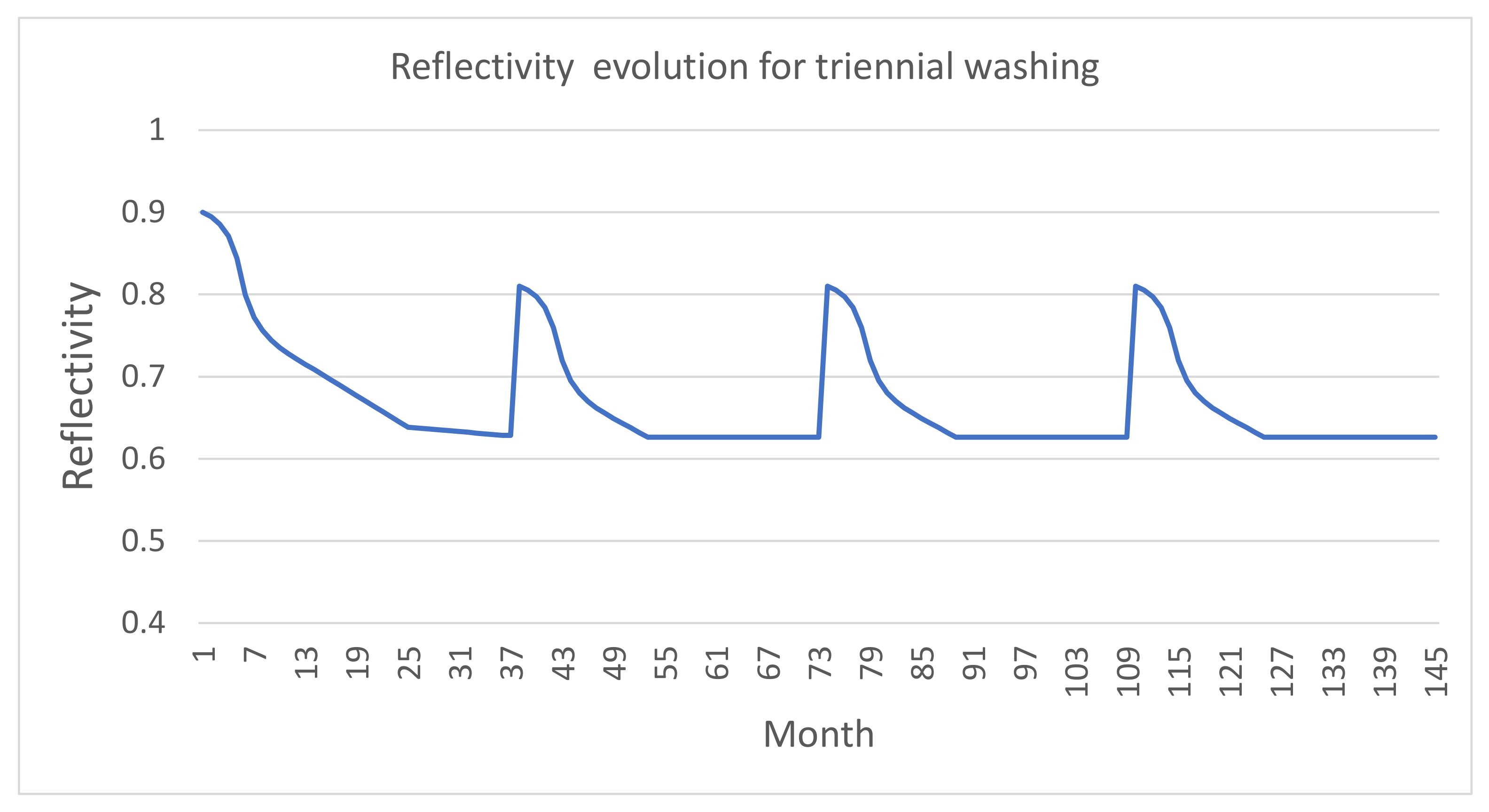
Finally, the pattern established in Reference [37] for the time evolution of the solar reflectivity, that collects the foregoing, is used in the computations. This pattern is illustrated in Figure 1 and Figure 2. In Figure 1, the evolution of the solar reflectivity of a cool roof with an initial value equal to 0.9 is shown for a triennial washing maintenance.

In Figure 2a, the monthly and accumulated loss of the solar reflectivity is shown for a period of 42 months, and, in Figure 2b,c, the assumed evolution of the solar reflectivity without maintenance and for a decennial washing, respectively, are shown for a period of 20 years.

An immediate consequence of the evolution over time of the exterior reflectivity is the need to calculate the heat transfer through the roof on a monthly basis for the whole LCA timespan. For this, the reflectivity value in Equation (2) must be updated for each moment of time, following the aging pattern described above. That is, the heat transfer through the roof cannot be considered the same for all the years of the LCA timespan, which is a frequent assumption in the literature.

2.3. Thermal Load Calculations

The key point of the developed analysis is the accurate computation of the heat transfer through the roof to the building indoor and the associated thermal loads to obtain indoor comfort. To do that, the load at time t is calculated using the expression entered above:

$$q\left(t\right)=h_{cr,int}(T\left(t\right)-T_{room})\left({\mathrm{W}/\mathrm{m}}^2\right),$$

(7)

which takes into consideration the convective and radiant thermal flux from the internal roof surface to the building indoor. $q\left(t\right)$ yields positive values when the heat flux enters to the building, and negative values when heat flows out of the building.

Then, if weather hourly values are considered, as it is usual in building energy software, the hourly load is derived from (7) for every hourly interval. This way, daily, monthly, and yearly loads are straightforwardly obtained by integrating the hourly loads on the timespan of interest.

The thermal loads due to the heat transfer through the roof, including the cooling and heating loads, are computed varying the absorptivity of the cool paint from $0.1$ to $0.5$, with this being the usual value range to consider a roof as a cool roof [51]; for computations, steps equal to 0.1 are considered for the absorptivity. The insulation thickness ranges from 0 to 10 cm, with the latter being the maximum value usually used for the roof retrofitting in southern Spain. For the computations, steps of 1 cm for the thickness of the insulation layer are considered.

We assume a fixed value of the indoor temperature in each season of the year. The conditioning system is considered to be in continuous mode with a fixed temperature set point at 24 ${}^{\circ }$C in the cooling season, at 20 ${}^{\circ }$C in the heating season, and at 22.5 ${}^{\circ }$C for the intermediate seasons, according with the comfort temperatures established in the Spanish regulations for thermal installations in buildings [52].

In order to estimate the energy loads due exclusively to the heat transfer through the roof, we follow the approach from References [4,31,53], and, then, the zone beneath the roof is assumed to have the envelope adiabatic, except for the roof.

The input data needed to compute the thermal loads are:

• Meteorological data: Air temperature, solar radiation, cloud cover, wind speed, and relative humidity. These data can be hourly or any other frequency smaller than one hour.
• Roof data: solar and thermal reflectivity of the outer roof surface and geometrical and thermophysical properties of the roof layers.
• Indoor data: indoor air temperature.

On the other hand, with regard to the aim of assessing the energy and economic performance of the refurbishment measure through the lifetime period of 20 years according to the service time of the roof coating, taken into consideration is the effect stemming from the action of environmental agents as rain, dust, air particles, moisture, or sun, as well as their own aging, on the initial reflectivity properties of the cool paint, as described in Section 2.2.

To estimate the thermal loads, the following cool coating maintenance scenarios were analyzed: no washing, and decennial, quinquennial, and triennial washing. Taking into account the social character of the buildings in which the roof reform is applied, it seems appropriate to consider an annual roof wash unlikely; realistically, only no maintenance, or washing every five or ten years, scenarios should be considered.

The thermal loads were estimated using the open source FreeFem++ software [54]. Hourly loads, including heating and cooling loads, were computed for the whole LC time interval.

2.4. Case Study

The case study considered is a building in the city of Seville. The city is located in the Guadalquivir valley in southern Spain; see Figure 3.

Its location in a valley with a low altitude above the sea, its meridional latitude, and its dry climate, together with the high levels of solar radiation, cause a long hot season, spanning months beyond summer which, together with its soft winters, make this city an appropriate place for the application of cool roofing techniques.

The climatic chart of Seville is shown in Figure 4 from data from the Spanish State Meteorological Agency [55]. The average annual temperature is 19.2 ${}^{\circ }$C, with maximum average temperatures up to 40 ${}^{\circ }$C in the months of July and August and a minimum average of 5.7 ${}^{\circ }$C in January. The normal incident solar radiation reaches a maximum daily mean equal to 8.3 kWh/m${}^2$ in July and a minimum daily mean equal to 2.3 kWh/m${}^2$ in December. Winters are mild while summers are warm, dry, and sunny. On the other hand, autumns and springs are characterized both by moderate temperatures and by being the seasons in which most of the rainfall occurs. According to the described characteristics, the studied area climate is classified as Mediterranean, following the Köppen-Geige climate classification.

It is noteworthy to observe the temperature differential between the temperature of the sky and the ambiance temperatures. As can be noted in Figure 4, this difference is up to 15 ${}^{\circ }$C throughout the year with respect the mean ambiance temperature, which is an indicator of the potential of the longwave heat exchange with the sky to reduce the roof surface temperature.

The studied building belongs to a quarter of social housing called La Juncal Figure 5 built in the sixties of the last century that exhibits the constructive characteristics common in the social housing built in Seville before 1979, when the first Spanish legislation designed to regulate energy demand in buildings was enacted.

In Figure 6a, the layout of a typical roof belonging to the social housing studied is shown, and, in

Table 1. Thermophysical characteristics of the reference roof.

Layer	Description	Thickness (m)	Density (kg/m3)	Specific Heat (J/kg K)	Conductivity (W/m K)
1 (Out.)	Ceramic tiles	0.005	2000	800	1.00
2	Mortar	0.01	2000	1000	1.40
3	Protective Layer	0.015	1150	1000	0.23
4	Mortar	0.01	2000	1000	1.40
5	Carbon cinders	0.1	640	657	1.40
6	Concrete vault	0.3	1330	1000	1.32
7 (Ins.)	Gypsum plaster	0.01	1000	1000	0.32

, the dimensions and thermophysical values of the components of the roofs are reported. This constructive configuration for roofs is the usual in the social housing built in the sixties of the past century at southern Spain [56]. For the outer surface of the roof, the absorptivity solar radiation value is taken equal to 0.8, with the latter being a typical value of the material making up this layer. This roof will henceforth be called the reference roof.

2.5. Energy Saving Refurbishment Measures

In order to improve the energy performance of the reference roof, a combined refurbishment measure was applied to the outside layer of the roof. This measure consisted of the installation of an EPS insulation and the application of an external layer of white elastomer cool paint to the outer surface. In Figure 6b, the layout of the retrofitted roof is shown, and, in

Table 2. Thermophysical characteristics of the refurbished roof.

Layer	Description	Thickness (m)	Density (kg/m3)	Specific Heat (J/kg K)	Conductivity (W/m K)
1(Out.)	White elastomer	0.0015	1150	1000	0.23
2	Regularization layer	0.01	2000	1000	1.40
3	EPS	0 to 0.1	30	1210	0.04
4–10 (Ins.)	Same as layers 1 to 7 of the reference roof (Table 1)

, the dimensions and thermophysical values of the components of the retrofit are reported. The combination of the insulation thickness and the value of the cool paint absorptivity is then analyzed to optimize the energy and economical performance of the roof, taking into consideration the time variation of the cool coating reflectivity discussed above.

2.6. Model Validation

In order to verify the reliability of the numerical model used in the present study, a twofold process of validation is performed: first, the model outputs are compared to the experimental values obtained from the monitoring of a full-scale outdoor test cell; and, second, the calculated values from the numerical model are compared to the values provided by a well known and validated building energy simulation (BES) tool, EnergyPlus, when applied to the case-study used here and described in Section 2.4.

The indices used to check the reliability of the numerical model were the root mean square error (RMSE), the mean of the residuals ${\epsilon }_{mean}$, the standard deviation of the residuals $SD\left({\epsilon }_{mean}\right)$, and the $r^2$ index, which are often used in the process of validation of building energy simulation models [57].

For both validation procedures, a winter week, from 7 to 14 February 2017, and a summer week, from 17 to 24 August 2017, were considered. The climatic data for both weeks were local data recorded by a meteorological station placed on the roof of a test cell in the city of Seville, as explained in Section 2.6.1. The indoor conditions assumed for the thermal load calculations, as in Section 2.3, are considered: An ambient interior temperature kept constant to 20 ${}^{\circ }$C in the winter week, and to 24 ${}^{\circ }$C in the summer week. In Figure 7, the ambiance temperature and solar radiation for both weeks are shown.

2.6.1. Experimental Validation

For the experimental validation, an outdoor full-scale test cell placed in the center of the city of Seville was used. The interior dimensions of the test cell are 2.40 m wide, 3.20 m deep, and 2.70 m high. The thermophysical values of the materials and the roof stratigraphy are presented in

Table 3. Thermophysical characteristics of the roof materials.

Layer	Description	Thickness (m)	Density (kg/m3)	Specific Heat (J/kg K)	Conductivity (W/m K)
1(Out.)	Galvanized corrugated
	sheet panels	0.002	7800	460	50.2
2	Ventilated air chamber	0.200	1.184	1007	0.0255
3	Sandwich panel	0.200	40	1884.15	0.017
2	Wool rock panel	0.160	100	840	0.046
3(In.)	Sandwich panel	0.100	40	1884.15	0.017

. The values shown in the table are the nominal ones provided by the Spanish Technical Building Code [58] and the material specifications sheets from the manufacturers. The outer surface of the roof is painted red, and a solar absorptivity of 0.5 and a thermal emissivity of 0.9 are considered for it.

The test cell is fully instrumented to measure the temperatures of the internal surfaces of the envelope, and data are recorded every 10 min. Thermocouples with an accuracy of ±0.75 ${}^{\circ }$C and an operating range of $-250$ to 350 ${}^{\circ }$C are used to monitor the temperature of the inner surfaces. Finally, a local meteorological station located on the roof of the cell is used to record weather data. More details on the test cell and its monitoring equipment can be found in Reference [59].

In

Table 4. Statistical indicators for the experimental validation.

	RMSE (${}^{\circ }$C)	${\mathit{\epsilon }}_{\mathbf{mean}}$ (${}^{\circ }$C)	$\mathbf{SD}\left(\mathit{\epsilon }\right)$ (${}^{\circ }$C)	${\mathit{r}}^2$
Winter	0.293	0.179	0.213	0.955
Summer	0.301	0.251	0.309	0.961

, the values of the statistical indices computed for the temperature of the inside roof surface, are shown.

The results obtained for the indicators shown in Table 4 allow for asserting that the presented model is able to compute the temperatures of the internal roof surface with good precision; the values obtained for the different indicators are similar to those obtained in other works for the validation of energy numerical models for a building’s envelope [57].

2.6.2. Comparison with EnergyPlus Software

The EnergyPlus [60] software is a well known BES tool that has been widely used for the calculation of the energy performance of buildings, proven to be very efficient in the computation of the thermal behavior of buildings. An example of the application of EnergyPlus to the analysis of the thermal behavior of roofs can be found in Reference [31].

To carry out the comparison between the numerical model presented here and the EnergyPlus tool, the reference roof of the case study in Section 2.4 and described in Table 1 is used, and the values for the temperature of interior roof surface provided by EnergyPlus are considered as benchmark.

In

Table 5. Statistical indicators for the comparison with EnergyPlus.

	RMSE (${}^{\circ }$C)	${\mathit{\epsilon }}_{\mathbf{mean}}$ (${}^{\circ }$C)	$\mathbf{SD}\left(\mathit{\epsilon }\right)$ (${}^{\circ }$C)	${\mathit{r}}^2$
Winter	0.263	0.084	0.107	0.985
Summer	0.287	0.121	0.226	0.981

, the values of the statistical indices computed for the temperature of the indoor roof surface, are shown.

The values of the indices shown in Table 5 allow to stablish the good fit between the values from the numerical method and from the EnergyPlus tool. As in the case of the experimental validation, these values are similar to those obtained in other validation processes of numerical thermal models for building envelopes [57]. On the other hand, it can be observed that the indicators for the comparison between the models have a slightly better performance than for the experimental validation, a fact also reported in the literature.

3. Energy Optimization Analysis

In this section, an analysis of the energy performance of a variety of roof solar reflectivity and insulation thickness combinations is carried out. The objective of this section is to determine the combination that provides the minimum energy consumption for the whole LCA timespan and to calculate the energy savings of each combination when compared to the reference case.

The analysis is carried out considering a time dependent change of the cool coating solar reflectivity due to the aging effect and different maintenance patterns, as described in Section 2.2.

The solar absorptivity of the cool coat varies from 0.1 to 0.5, with steps equal to 0.1. The insulation thickness ranges from 0 to 0.1 m, with steps equal to 0.1. For the outer surface of the retrofitted and the reference roofs, the thermal emissivity taken is equal to 0.9. The considered maintenance for the cool roof was a power washing every three, five, or ten years. The case where no power washing is performed was also included in the analysis.

The transmission loads through the roofs are calculated for the entire LC timespan taking into account the annual variability of the thermal loads during that period of time due to the changes in time of the cool layer reflectivity produced by the effects of aging and maintenance patterns.

3.1. Thermal Loads Results

In Figure 8 and Figure 9, the total thermal loads (cooling plus heating loads) for the whole LC timespan are shown for different values of solar absorptivity, thickness insulation, and maintenance protocols, together with the total load for the reference roof. As can be seen in these figures, the effect of low absorptivity values on the total thermal loads is very noticeable as it is observed when comparing with the reference case, even in the case of the retrofitted roof without insulation. For all the combinations and all maintenance protocols considered, the total loads are lower than for the reference case, although there is a significant difference between the loads for the uninsulated roof and the insulated ones.

On the other hand, it is observed that the lower the solar absorptivity, the lower is the total load. It is also observed that increasing the thickness of the insulation reduces the loads. So, for every value of the solar absorptivity, the total load decreases as the insulation thickness increases. However, regarding the maintenance protocol, only little differences are found among the total loads, with a slight tendency to decrease as the frequency of the cool coat washes increases. Thus, it can be drawn up that the role played by periodic washing in the total thermal loads is relatively modest.

Analyzing the heating and the cooling loads separately, it is clear that, for all the cases of absorptivity, thick insulation, and maintenance protocols, the smaller the cool roof absorptivity, the smaller the cooling load, as can be seen in Figure 10 and Figure 11. In addition, it can be noted that the smallest cooling loads are obtained for the case of the triennial wash, which is in accordance to the fact that the original roof solar absorptivity values are restored with a higher frequency than in the other maintenance protocols. Therefore, the cooling loads gradually increase as the frequency of cool roof maintenance decreases and reaches the highest values for the case of no power washing.

On the other hand, it can be seen that increasing the thickness of the insulation has a strong effect in reducing the cooling loads, so that the thicker the insulation layer, the lower the cooling load. It can be concluded that, for all the maintenance protocols, the lowest load is obtained for the thickest insulation and the lowest solar absorption. Regarding the maintenance protocol, the most favorable case is the triennial power washing.

Regarding the heating loads, the behavior is the opposite to that described for the cooling loads, as can be observed in Figure 12 and Figure 13. Now, due to solar gains decrease, the retrofitted cool roof without insulation has higher heating loads than the reference case. Clearly, the winter penalty effect on solar gains due to the cool roof is the cause of this. For the roofs with insulation, the only case where the heating loads are greater or close to that of the reference roof is when solar absorptivity equals 0.1. For values greater than 0.1 of the roof absorptivity, the heating loads are lower when compared to the reference case. This result holds for all the insulation thickness and maintenance protocols. Therefore, it can be stated that, although the heating loads increase as the solar absorptivity of the roof decreases, the insulating layer is able to compensate the penalty effect due to the low values of absorptivities, except for the value of the absorptivity equal to 0.1, as discussed before. Again, the role of the insulation layer in reducing the heat flux is obvious, i.e., the thicker the insulation, the lower the heating load. Finally, it is again observed that the effect of the cool coat washing is quite small on the heating loads over the LC timespan.

This opposite behavior of the heating and cooling loads described for the retrofitted roofs is the cause of the small differences observed among the total thermal loads for the whole LC timespan when considering different maintenance scenarios, while the changes in solar reflectivity produced by the aging of the cool coat act in the opposite direction. That is, on the one hand, when power washing is carried out, it produces a decrease in the cooling loads and an increase in the heating loads, while the aging of the cool coat produces the opposite effect in such a way that all these processes combined they result in a certain equilibrium in the resulting total loads. To take into account the aging of the cool coat, the aging pattern discussed in Section 2.2 is used for the thermodynamic computations by using the monthly reflectivity given by the pattern.

In Figure 8 and Figure 9, the most remarkable fact, from a physical point of view, is the difference between roofs equipped with thermal insulation and roofs without it; this is due to the higher heat flux values through roofs without thermal insulation, which implies, in the cold season, a greater loss of heat from the interior and, in the hot season, a greater gain, so that these effects produce a significant thermal load increasing for the roofs without insulation when compared to the equipped with insulation ones. On the other hand, it can be observed that, for the roof without insulation, the reduction of heat gain due to the solar reflective coat compensates the penalty effect on winter; this means that the reduction of thermal conduction through the roof in summer, due to the lower absorption of solar radiation, compensates, in terms of energy consumption to obtain indoor comfort, the increase in energy consumption necessary to achieve indoor comfort conditions in winter, due to the aforementioned lower absorption of solar radiation. This effect is clear in Figure 10, Figure 11, Figure 12 and Figure 13, where it can be observed the strong reduction in cooling loads for the roof with cool coat without insulation when compared to the reference case, while, regarding the heating loads, although higher for the reference roof, it has a lower difference on thermal loads when compared to the cool roof; this difference is collected by the total load, which, as said before, is lower for the roof with cool coat.

On the other hand, noteworthy is the energy performance of the roofs with insulation. These roofs are able of reducing thermal conduction in both directions, from inside to outside and vice versa, which produces a significant reduction in thermal loads compared to roofs without thermal insulation, as can been observed in Figure 8 and Figure 9. It is observed, in Figure 10, Figure 11, Figure 12 and Figure 13, that the higher the thickness of the insulation layer, the less the thermal loads, for both cooling and heating, which is in accordance with the reduction of heat transfer through the roof caused by the insulation layer. On the other hand, as expected, it can be observed the progressive reduction of the cooling loads as the solar absorptivity increases, obviously due to the decreasing solar radiation absorbed by the roof, whilst, for the same reason, the opposite is observed for heat loads. However, what is concluded, as it is shown in Figure 8 and Figure 9, is that, for the climatic conditions and the geographical framework in which the study has been developed, the total load decreases as the reflectivity increases due to the fact that the reduction in thermal flux to the interior achieved in summer, and which impacts on cooling loads, is greater than the increase in thermal flux from the inside to the outside, which occurs in winter, and that is reflected in an increase in heating loads.

3.2. Energy Optimization Results

This section studies the optimum combination of solar reflectivity and insulation thickness in terms of thermal loads for the entire LC time interval. Energy savings of the different combinations when compared to the reference case are also reported.

From the results shown in Figure 8 and Figure 9, it can be concluded that the optimum combination to reduce energy consumption is absorptivity equals 0.1, and insulation thickness equals 0.1. This result holds for all the maintenance scenarios, although the results for the different maintenance scenarios are very close to each other. To clarify this, in

Table 6. Total loads (GJ/m${}^2$) for the LC timespan.

	No Washing					Decennial Washing
Insulation Thickness	Abs. = 0.1	Abs. = 0.2	Abs. = 0.3	Abs. = 0.4	Abs. = 0.5	Abs. = 0.1	Abs. = 0.2	Abs. = 0.3	Abs. = 0.4	Abs. = 0.5
0.0	5.0350	5.1889	5.3882	5.6335	5.9216	4.9544	5.0798	5.2491	5.4632	5.7190
0.03	2.2712	2.3156	2.3802	2.4625	2.5619	2.3458	2.3863	2.4477	2.5328	2.6110
0.05	1.7131	1.7459	1.7939	1.8426	1.9414	1.7470	1.7480	1.7929	1.8551	1.9163
0.07	1.3835	1.4121	1.4527	1.5012	1.5671	1.3749	1.4066	1.4459	1.4984	1.5588
0.1	1.0802	1.1307	1.1329	1.1745	1.2188	1.0797	1.1010	1.1281	1.1729	1.2136

and

Table 7. Total loads (GJ/m${}^2$) for the LC timespan.

	No Washing					Decennial Washing
Insulation Thickness	Abs. = 0.1	Abs. = 0.2	Abs. = 0.3	Abs. = 0.4	Abs. = 0.5	Abs. = 0.1	Abs. = 0.2	Abs. = 0.3	Abs. = 0.4	Abs. = 0.5
0.0	4.9678	5.0592	5.1993	5.3884	5.5577	4.9206	4.9981	5.1178	5.2813	5.4856
0.03	2.3884	2.4287	2.4850	2.5645	2.6415	2.3483	2.3967	2.4519	2.5255	2.6184
0.05	1.7802	1.7655	1.8028	1.8538	1.9162	1.7679	1.7456	1.7813	1.8244	1.8959
0.07	1.3835	1.4135	1.4507	1.5016	1.5618	1.3662	1.3943	1.4319	1.4805	1.5467
0.1	1.0763	1.1103	1.1349	1.1760	1.2168	1.0634	1.0970	1.1220	1.1628	1.2056

, the values of the total thermal loads for the LC timespan are shown.

The similarity of the loads among the different maintenance protocols for the cool roof can be observed in all those cases for which the absorptivity values and the thickness of the insulation layer are the same. Note that, for the optimum combination established, the total thermal load difference between the optimum maintenance scenario, i.e., triennial washing, and the worst scenario, i.e., no washing, is only of 0.01676 GJ/m${}^2$, equivalent to a $1.55\%$ difference.

In

Table 8. Total load savings (GJ/m${}^2$) for the LC timespan.

	No Washing					Decennial Washing
Insulation Thickness	Abs. = 0.1	Abs. = 0.2	Abs. = 0.3	Abs. = 0.4	Abs. = 0.5	Abs. = 0.1	Abs. = 0.2	Abs. = 0.3	Abs. = 0.4	Abs. = 0.5
0.0	2.1181	2.0553	1.9157	1.7359	1.5171	2.0992	2.0029	1.8623	1.6835	1.4685
0.03	4.6168	4.5724	4.5078	4.4255	4.3261	4.5960	4.5474	4.4806	4.3907	4.3049
0.05	5.1749	5.1421	5.0941	5.0454	4.9466	5.1816	5.1463	5.0955	5.0261	4.9663
0.07	5.5045	5.4759	5.4353	5.3868	5.3209	5.5084	5.4781	5.4402	5.3910	5.3296
0.1	5.8078	5.7573	5.7551	5.7135	5.6692	5.8083	5.787	5.7599	5.7229	5.6753

and

Table 9. Total load savings (GJ/m${}^2$) for the LC timespan.

	No Washing					Decennial Washing
Insulation Thickness	Abs. = 0.1	Abs. = 0.2	Abs. = 0.3	Abs. = 0.4	Abs. = 0.5	Abs. = 0.1	Abs. = 0.2	Abs. = 0.3	Abs. = 0.4	Abs. = 0.5
0.0	2.1020	2.0138	1.8900	1.7277	1.5865	2.0561	1.9863	1.8642	1.6970	1.4892
0.03	4.5870	4.5369	4.4731	4.3868	4.3050	4.5851	4.5355	4.4786	4.4035	4.3206
0.05	5.1739	5.1433	5.0979	5.0343	4.9684	5.1548	5.1404	5.1013	5.0462	4.9750
0.07	5.5064	5.4790	5.4444	5.3963	5.3328	5.4995	5.4789	5.4482	5.4048	5.3446
0.1	5.8117	5.7777	5.7531	5.7270	5.6806	5.8246	5.7910	5.7663	5.7300	5.6862

, the savings for the total thermal loads of every retrofitted roof when compared to the reference roof are shown. In accordance with the energy results presented above, all the combinations are found to provide energy savings compared to the reference case.

From the above, it is straightforward that the greatest energy savings are obtained by the retrofitting combination that uses a cool roof with an absorptivity equal to 0.1 and an insulation layer thickness equal to 0.1 m, with the triennial washing of the cool coat being the case that gives the highest energy saving; on the other hand, the energy savings decrease as the absorptivity increases, and the insulation thickness decreases, according to the previous discussion on thermal loads.

4. Cost Optimization Analysis

The objective of this analysis is to assess the cost-effectiveness of the energy retrofitting measures proposed when compared to the reference case, as well as to find out the combination of cool coating reflectivity and insulation layer thickness that yields the minimum LC cost under the climate conditions considered.

The optimum combination of cool coating reflectivity and insulation thickness is a function of the costs of the cool paint and the insulation material, the application of the cool paint, the insulation layer installation, the cool coat maintenance, the thermal loads due to the energy transfer through the roof, the coefficient of performance (COP) of the heating and cooling systems, the retrofitting materials lifetime, the energy prices, the energy inflation rate, and the monetary discount rate.

Despite the aforementioned tendency of heating and cooling loads to decrease when the thickness of the insulation layer increases, a rise in the reflectivity of the cool coat tends to reduce the cooling load, as well as the solar gain, in winter. Furthermore, the aging and the washing of the cool coat give rise on their own to contrary effects on the loads. So, this time-varying evolution of the thermal loads, combined with the effect of the costs of the retrofitting material and its maintenance, makes it necessary to carry out a detailed analysis of the combined effect on the LCA cost of the different retrofitting combinations in order to obtain the optimum results. The main difference between the present analysis and the usual cost analysis is that, here, the costs are computed monthly for the whole LC time interval, with the goal of assessing the effect on the evolution of costs, along time, produced by changes in the thermal loads associated to the cool coat reflectivity variation, throughout the LC timespan.

4.1. Methodology

First, the assessment of the cost-effectiveness of every ESRM is done. To that aim, the methodology from Reference [61] is used. This methodology performs an LCCA, where all anticipated costs are estimated and discounted to their present worth.

The procedure consists in computing the costs for each future time period using the future value of the variables involved and then discounting each future cost to its present worth. Thereby, the sum of all the present values of the costs yields the life-cycle cost.

Once the LC cost has been determined for each of the considered ESRMs, including different scenarios for maintenance, the cost-effectiveness of each case is assessed by its LC cost: the lower this cost, the more cost effective the ESRM, and the one having the lowest LC cost is selected as the optimum.

The lifetime for the life-cycle analysis is taken as equal to $n=20$ years, which is the mean service life of the used cool coat and the insulation material [62]. Then, for every considered ESRM, the life-cycle cost, the associated savings, and the payback period are computed.

In the present LCCA, the method P1-P2 introduced in Reference [61] is used with some little changes to account for the time changing character of the energy operating costs associated to the variation of the cool coat solar reflectivity due to the aging and washing of the coat. We use the expression

$$P{W}_k=1/{(1+d)}^k$$

(8)

to compute the present worth ($PW$) of one monetary unit belonging to the future time interval k (usually years), where d is the market discount rate (fraction per time period).

In the present analysis, k, for $k=1,\dots ,n$, is taken as the year in which the costs are being computed. Then, if we note as $Q_c\left(k\right)$ and $Q_h\left(k\right)$ the cooling and heating loads at year k for each ESRM, the energy payment for the whole year k is given by:

$$C_e\left(k\right)=\left(\frac{Q_c\left(k\right)\times P_{e,c}}{CO{P}_c\times (3.6\times {10}^6)}+\frac{Q_h\left(k\right)\times P_{e,h}}{CO{P}_h\times (3.6\times {10}^6)}\right){(1+i)}^{k-1},$$

(9)

where $P_{e,c}$ and $P_{e,h}$ are the current prices of energy used to cool and heat for cooling and heating, respectively, $CO{P}_c$ and $CO{P}_h$ are the coefficients of performance for cooling and heating, and, finally, i is the considered inflation rate for energy costs.

Then, in accordance with expression (8), the present worth of the future energy payment $C_e\left(k\right)$ at the period k is given by

$$P{W}_k\left(C_e\left(k\right)\right)=C_e\left(k\right)/{(1+d)}^k.$$

It is noteworthy that, although $C_e\left(k\right)$ represents the energy costs for year k, it is computed by taking into account the changing values of energy consumption for every specific year k according to the monthly changes in the solar reflectivity of the cool coat.

To compute $C_e\left(k\right),$ the energy source considered for cooling is electricity, while, for heating, the use of electricity or gas have been considered, given that they are the usual sources of energy used in the geographical framework under analysis.

To include the maintenance in the cost computation, we name as $i_M$ the inflation rate for this kind of costs. Then, again applying (8), the present worth of the future maintenance payment $C_M\left(k\right)$ at the period k is given by

$$P{W}_k\left(C_M\left(k\right)\right)=C_M\left(k\right)/{(1+d)}^k=\delta \left(k\right)C_M{(1+i_M)}^{k-1}/{(1+d)}^k,$$

where $C_M$ is the current price of maintenance per unit area of roof surface, and $\delta \left(k\right)$ is defined as:

$$\delta \left(k\right)=\left\{\begin{array}{cc}1,\hfill & \mathrm{i}\mathrm{f} \mathrm{t}\mathrm{h}\mathrm{e} \mathrm{m}\mathrm{a}\mathrm{i}\mathrm{n}\mathrm{t}\mathrm{e}\mathrm{n}\mathrm{a}\mathrm{n}\mathrm{c}\mathrm{e} \mathrm{i}\mathrm{s} \mathrm{d}\mathrm{o}\mathrm{n}\mathrm{e} \mathrm{a}\mathrm{t} \mathrm{p}\mathrm{e}\mathrm{r}\mathrm{i}\mathrm{o}\mathrm{d} \mathit{k};\hfill \\ 0,\hfill & \mathrm{i}\mathrm{f} \mathrm{t}\mathrm{h}\mathrm{e} \mathrm{m}\mathrm{a}\mathrm{i}\mathrm{n}\mathrm{t}\mathrm{e}\mathrm{n}\mathrm{a}\mathrm{n}\mathrm{c}\mathrm{e} \mathrm{i}\mathrm{s} \mathrm{n}\mathrm{o}\mathrm{t} \mathrm{d}\mathrm{o}\mathrm{n}\mathrm{e} \mathrm{a}\mathrm{t} \mathrm{p}\mathrm{e}\mathrm{r}\mathrm{i}\mathrm{o}\mathrm{d} \mathit{k}.\hfill \end{array}\right.$$

Then, the present worth of the energy total cost for the life-cycle timespan is computed as $C_e={\sum }_{k=1}^{n}P{W}_k\left(C_e\left(k\right)\right)$, whilst the present worth value of maintenance life-cycle total cost is computed as $C_M={\sum }_{k=1}^{n}P{W}_k\left(C_M\left(k\right)\right).$ Now, if we note as $C_{I,cc}$ and $C_{I,ins}$ the initial costs of installation of the cool coat and the insulation layer, the total initial cost for installation is given by $C_I=C_{I,cc}+C_{I,ins}$. Finally, the present worth of the life-cycle total cost per unit area for each considered ESRM and maintenance scenario is given by:

$$C_t=C_e+C_M+C_I.$$

Once $C_t$ is computed for every case, the optimum case is considered to be the one that yields the lower value for $C_t$.

On the other hand, to compute the possible savings of the proposed ESRMs, the $PW$ of the LC total cost must be estimated for the reference case, too. Then, the $PW$ of the energy costs for the reference case at period k, $P{W}_k\left(C_e^{\left(ref\right)}\left(k\right)\right)$, is computed by:

$$P{W}_k\left(C_e^{\left(ref\right)}\left(k\right)\right)=C_e^{\left(ref\right)}\left(k\right)/{(1+d)}^k,$$

where $C_e^{\left(ref\right)}\left(k\right)$ is the energy future cost at period k for the reference roof calculated by:

$$C_e^{\left(ref\right)}\left(k\right)=\left(\frac{Q_c^{\left(ref\right)}\left(k\right)\times P_{e,c}}{CO{P}_c\times (3.6\times {10}^6)}+\frac{Q_h^{\left(ref\right)}\left(k\right)\times P_{e,h}}{CO{P}_h\times (3.6\times {10}^6)}\right){(1+i)}^{k-1},$$

(10)

with $Q_c^{\left(ref\right)}\left(k\right)$ and $Q_h^{\left(ref\right)}\left(k\right)$ being the cooling and heating loads, respectively, for the reference roofs at the time period k.

Now, we note by $C_I^{\left(ref\right)}$ and $C_M^{\left(ref\right)}$ the installations and maintenance costs, respectively, of the minimum retrofitting action to be done on the reference roof and which is deemed to be the bituminous paint retrofitting.

Then, the difference between the costs for the cool roofs and the reference case for the whole LC period is estimated through the net savings (NS):

$$NS=\sum _{k=1}^n\left[P{W}_k\left(C_e^{\left(ref\right)}\left(k\right)\right)-P{W}_k(C_e\left(k\right)\right]+(C_M^{\left(ref\right)}-C_M)+(C_I^{\left(ref\right)}-C_I).$$

(11)

A positive value for $NS$ means that the use of the ESRM under consideration yields economic savings when compared to the reference case and that the retrofitting system is cost-efficient. Due to the outlined thermal loads change over time, the net savings (11) cannot be reduced to a simple analytical expression, and its computation must be performed through the yearly computation, according to the yearly changes in thermal loads; this represents a distinguishing feature of our analysis with respect to the usual analysis of cost-effectiveness for retrofitting measures found in the literature.

To compute the period of investment return or payback period (PB), we follow Reference [63] and take PB as the time horizon t, for which the value of NS becomes zero. To compute this value of t, since the terms of the series in Equation (11) are not constant on k, the net savings accumulated for every time horizon $k_0$ is computed first:

$$NS\left(k_0\right)=\sum _{k=1}^{k_0}\left[P{W}_k\left(C_e^{\left(ref\right)}\left(k\right)\right)-P{W}_k(C_e\left(k\right)\right]-C_M-C_I.$$

(12)

Then, if $NS\left(k_0\right)<0$ and $NS(k_0+1)>0$, the value of the payback period t is estimated as:

$$t=\frac{-NS\left(k_0\right)}{NS(k_0+1)-NS\left(k_0\right)}+k_0.$$

(13)

The value of t given by (13) is consistent with the value provided by the usual formulas for the PB found in the literature used under the consideration of constant energy consumption for all the years of the LC period [31,61]. In Appendix C, a comparison between the formula given by (13) and the formula for the computation of the PB from References [31,61,63] is performed.

4.2. Variables for the LCA Economic Analysis

The input variables needed to carry out the economic calculations involved in the LCCA are shown in

Table 10. Input variables used in the LCA.

Variable	Value
EPS cost	116	€/m${}^3$
Insulation installation cost	13.15	€/m${}^2$
Cool paint cost	9.45	€/m${}^2$
Washing cost	1.63	€/m${}^2$
Bituminous paint cost	8.01	€/m${}^2$
Bituminous paint maintenance	0.4	€/m${}^2$ yearly
Electricity cost	0.2403	kWh
Gas cost	0.0736	kWh
Energy inflation rate	$3$	%
Discount rate	$1.5$	%
Lifetime	20	years

.

The costs of the cool and bituminous paint application, their maintenance, and the insulation material and its installation are taken from Reference [62]. The electricity and natural gas prices are the average final prices for household consumers in Spain during the year 2020 as reported by Eurostat Office [64]. The values of the energy inflation and the discount rates have been taken considering the average values of these parameters under Spanish and European economic conditions, with such values being previously used for the LCA cost analysis in former research [37,65]. Regarding the conditioning equipment, it has been considered that cooling is always done by air conditioning machinery using electricity as the only energy source, while, for heating, we have considered the following cases:

• Heating by air (heat pumps).
• Heating by natural gas.
• Heating by electricity radiators.

The machinery is considered common in the local market and it has a mid-range efficiency. The efficiency indices of the conditioning devices are listed in

Table 11. Conditioning equipment efficiency.

Device	Efficiency
Cooling pump	COP = 3.4
Heating pump	COP = 3
Gas natural heating	${\eta }_s$= 0.8
Electrical Radiators heating	${\eta }_s$= 1

.

4.3. Cost Optimization Results

In this section, the economic results from the LCCA for the considered ESRMs are shown. The objective of this analysis is twofold: first, the cost-effectiveness of the ESRMs will be assessed; second, the optimum case for the combination of insulation layer, roof solar absorptivity, and maintenance protocol will be determined.

The NS and PB were calculated by using the economic variables introduced in Section 4.1 and considering the aging and maintenance scenarios presented in Section 2.2. For each ESRM, a positive NS means real savings and, conversely, a negative NS implies that the ESRM has a higher LCA cost than the reference case and, therefore, no real savings. Finally, once $C_t$ is computed for every considered ESRM and for every cool roof maintenance protocol, the lowest value of $C_t$ determines the optimum combination.

On the other hand, the cost of the roof retrofitting must be paid by all the owners of the building, while the benefit of the retrofitting would only be noticeable in the housing under the roof; however, in the event of damage, according Spanish law, the cost of restoring the roof is paid by all the owners of the building; so, since the owners and tenants of the dwellings taken as the case study are characterized by having low incomes, a retrofitting action on the roof is unlikely, except for the existence of some deterioration of the roof that makes such retrofitting necessary; thus, to perform the analysis, it is assumed that the reference roof needs some kind of renovation or maintenance. This way, the application of a bituminous paint is chosen since this is considered to be the most usual retrofitting measure in the socioeconomic context within which the study is performed.

In

Table 12. Optimum results for cooling and heating by pump.

Cool Roof Washing	Solar Absorptivity	Optimum Thickness (m)	Minimum Total Cost (€/m${}^2$)	Maximum total Savings (€/m${}^2$)	Payback Period (Years)
No	0.1	0.08	64.27	109.94	4.54
Decennial	0.1	0.08	66.51	107.70	4.78
Quinquennial	0.1	0.08	68.33	105.88	5.01
Triennial	0.1	0.08	72.82	101.39	5.48

, the optimum values with regard to the use of pump for heating and cooling are shown for every protocol maintenance and for the whole LC timespan. These values have been extracted from

Table A4. Cooling and heating by pump. Total costs (/m${}^2$) for the LC timespan.

	No Washing					Decennial Washing
Insulation Thickness	Abs. = 0.1	Abs. = 0.2	Abs. = 0.3	Abs. = 0.4	Abs. = 0.5	Abs. = 0.1	Abs. = 0.2	Abs. = 0.3	Abs. = 0.4	Abs. = 0.5
0.0	129.32	131.66	135.21	139.77	145.31	132.30	134.28	137.93	142.46	146.94
0.01	104.76	106.01	109.27	112.66	125.55	104.83	106.54	109.11	113.82	126.63
0.02	91.35	92.55	95.02	98.21	105.23	93.93	95.91	98.07	103.17	106.63
0.03	83.51	84.56	86.30	88.32	90.90	85.40	86.49	88.21	90.57	92.53
0.04	77.20	78.04	79.69	80.97	83.69	78.83	79.98	81.05	83.92	84.63
0.05	71.74	72.58	73.80	74.87	77.01	73.39	73.83	75.03	76.49	78.64
0.06	67.14	68.94	70.11	71.55	74.82	69.77	70.08	71.79	72.26	75.63
0.07	64.61	66.01	67.41	68.96	70.41	67.07	67.92	68.63	69.93	72.03
0.08	64.27	65.40	66.49	67.71	68.82	66.51	67.10	67.71	68.74	69.63
0.09	64.47	64.78	65.16	65.73	66.01	66.67	67.21	67.53	67.60	67.63
0.1	64.81	64.86	64.95	65.03	65.11	67.08	67.41	67.64	67.71	67.74
	Quinquennial Washing					Triennial Washing
Insulation Thickness	Abs. = 0.1	Abs. = 0.2	Abs. = 0.3	Abs. = 0.4	Abs. = 0.5	Abs. = 0.1	Abs. = 0.2	Abs. = 0.3	Abs. = 0.4	Abs. = 0.5
0.0	135.76	138.16	141.76	146.01	150.50	140.60	143.02	146.13	149.32	153.54
0.01	106.21	109.31	112.66	116.03	120.76	109.76	112.83	116.21	119.96	124.15
0.02	95.38	96.85	98.22	100.92	103.76	98.82	100.23	101.97	104.08	106.49
0.03	88.20	89.77	90.18	92.37	94.88	92.16	93.55	95.19	97.28	98.68
0.04	80.86	82.10	83.56	84.98	86.52	85.15	85.20	86.62	88.21	89.91
0.05	76.15	76.69	77.81	79.02	80.31	79.96	80.64	81.75	82.73	84.07
0.06	71.74	72.39	74.10	75.22	76.81	75.79	76.60	77.59	78.39	79.11
0.07	69.37	70.10	71.22	72.46	73.74	73.74	74.43	75.37	76.24	77.04
0.08	68.33	68.39	68.46	68.78	68.99	72.82	73.19	73.58	73.90	74.38
0.09	68.40	68.55	68.61	68.83	69.11	72.89	73.26	73.81	74.21	74.61
0.1	68.72	68.71	68.89	69.38	69.57	73.11	73.39	74.07	74.48	74.71

in Appendix B, where all the LC total costs are shown for the different values of both the insulation thickness layer and the roof reflectivity, as well as for all the colorredconsidered roof maintenance protocols. For this case of considering electricity as the only energy source to conditioning, the estimated LC total cost for the reference case is equal to 174.21/m${}^2$. Then, this value is used to obtain the economic savings and the payback periods shown in the table.

As can be observed in Table 12, when a pump is used for heating and cooling, the cool roof absorptivity that provides the minimum total cost is equal to 0.1, and the insulation thickness is equal to 0.08 for all the maintenance scenarios. The optimum result is obtained for the non-maintenance scenario with a total cost equal to 64.27/m${}^2$, a total savings equal to 109.94/m${}^2$, and a payback period of 4.54 years.

In

Table 13. Optimum results for cooling by pump and heating by gas.

Cool Roof Washing	Solar Absorptivity	Optimum Thickness (m)	Minimum Total Cost (€/m${}^2$)	Maximum total Savings (€/m${}^2$)	Payback Period (Years)
No	0.1	0.08	68.27	111.80	4.05
Decennial	0.1	0.08	69.81	110.26	4.48
Quinquennial	0.1	0.09	71.30	108.77	4.71
Triennial	0.2	0.08	74.99	105.08	4.97

, the optimum values regarding the use of gas for heating and of a pump for cooling are shown for every protocol maintenance and for the whole LC timespan. These values have been sourced from

Table A5. Cooling by pump and heating by gas. Total costs (/m${}^2$) for the LC timespan.

	No Washing					Decennial Washing
Insulation Thickness	Abs. = 0.1	Abs. = 0.2	Abs. = 0.3	Abs. = 0.4	Abs. = 0.5	Abs. = 0.1	Abs. = 0.2	Abs. = 0.3	Abs. = 0.4	Abs. = 0.5
0.0	141.20	142.47	145.06	148.73	153.473	143.75	144.84	147.56	151.26	155.93
0.01	108.10	109.51	112.27	112.66	125.55	111.63	112.84	114.27	117.02	122.63
0.02	95.70	96.65	99.87	98.21	105.23	98.63	99.31	100.87	102.63	104.11
0.03	88.22	88.91	90.99	92.58	94.74	90.93	91.51	92.81	94.72	95.68
0.04	80.61	81.34	82.09	80.97	83.69	83.63	83.94	85.36	86.02	86.73
0.05	76.04	76.48	77.346	78.22	79.1	77.58	77.77	78.60	79.78	80.48
0.06	71.14	71.54	72.61	71.55	74.82	73.69	73.98	74.69	75.86	76.33
0.07	69.19	69.61	70.35	71.36	72.74	70.57	70.92	71.49	72.55	73.78
0.08	68.27	68.70	69.19	70.94	68.82	69.81	70.07	70.61	71.54	71.63
0.09	68.54	68.88	69.46	70.43	66.01	70.08	70.13	70.83	71.20	71.55
0.1	69.27	69.63	70.15	70.59	65.11	70.34	70.49	70.94	71.33	71.49
0.0	147.44	147.90	150.42	153.99	158.57	152.81	151.93	154.03	157.35	161.78
0.01	114.09	115.78	118.66	121.53	124.34	118.95	118.23	120.57	122.17	126.03
0.02	101.76	102.99	104.22	106.01	108.16	106.12	107.13	108.55	110.28	111.01
0.03	93.79	94.31	95.53	96.73	97.81	97.97	98.26	99.32	100.76	101.8
0.04	85.65	86.10	87.16	88.61	89.92	89.95	90.03	91.11	92.16	93.88
0.05	80.31	80.36	81.12	82.29	83.36	84.22	84.25	84.90	85.88	87.15
0.06	75.55	75.78	76.30	77.12	77.98	79.78	79.70	80.48	81.39	82.39
0.07	73.05	73.61	74.13	74.89	75.53	77.62	77.25	77.62	78.5	79.73
0.08	71.63	72.11	72.66	73.18	74.80	75.52	74.99	75.38	75.96	76.98
0.09	71.3	71.85	72.71	73.03	74.06	75.53	75.06	75.51	75.71	76.41
0.1	71.45	72.07	72.93	73.12	73.97	75.68	75.27	75.86	76.01	76.28

in Appendix B, where all the LC total costs are shown for the different values of both the insulation thickness layer and the roof reflectivity, as well as for all the roof maintenance protocols. Within the framework of this energy source for conditioning, the LC total cost for the reference case is equal to 180.07/m${}^2$. For the cases of no-maintenance and decennial maintenance, the combination that provides the maximum savings is that which has a solar absorptivity equal to 0.1 and an insulation thickness equal to 0.08, while, for the quinquennial maintenance, the combination yielding the maximum savings is that which has a solar absorptivity equal to 0.1 and an insulation thickness equal to 0.09 and, finally, for the triennial maintenance, the combination that provides the maximum savings is that which has a solar absorptivity equal to 0.2 and an insulation thickness equal to 0.09. For this scenario of mixed energy used to condition the building, the optimum result is also obtained for the non-maintenance scenario with a total cost equal to 68.27/m${}^2$, a total savings equal to 111.80/m${}^2$, and a payback period of 4.05 years.

In Figure 14, Figure 15, Figure 16 and Figure 17, the insulation cost, the cool coating cost (including maintenance), the energy consumption cost, and the total cost are displayed with respect to the insulation thickness for the optimum absorptivities shown in Table 12 and Table 13, for all the maintenance scenarios and for the two considered sources of energy.

As it can be seen from these figures, there is a rapid decrease in energy costs when the insulation thickness begins to increase from zero. This also results in a rapid decrease in total costs. However, for values of insulation thickness greater than 0.07 m, energy costs decrease at a much weaker rate according to the decrease in the rate of reduction of thermal loads. Thereby, the decrease in energy costs is not balanced by the increase in insulation costs, with this fact being much more evident for the higher frequency washing of the cool coating. This way, when using electricity as the only energy source for conditioning, the curve of total costs has a minimum for the insulation thickness equal to 0.08 m that corresponds to the optimum insulation thickness for all the cool roof maintenance cases; when using gas for heating and electricity for cooling, in the case of quinquennial cool roof maintenance, the optimum is reached for an insulation thickness equal to 0.09 m, whilst, for the cases of no-maintenance, decennial, and triennial cool roof maintenance, the curve of total costs exhibits a minimum for an insulation thickness equal to 0.08 m, even though, for the triennial maintenance, the minimum total cost is reached for a solar absorptivity equal to 0.2, as is shown in Table A5 in Appendix B.

As it can be observed in Table A4 and Table A5 in Appendix B, even if, as it is reported in the energy analysis, the minimum energy consumption was obtained for triennial washing when absorptivity equals 0.1 and insulation thickness equals 0.1 m, energy cost savings are not enough to compensate the rise of cost derived of the increase in insulation thickness and of the cool roof maintenance. On the other hand, as it is deduced from those tables, all the studied ESRMs are cost-effective and produce positive savings. This result holds for all the different cases of maintenance of cool roofs and of machinery for conditioning.

Thus, from the performed economic analysis, it can be concluded that the optimum combination is that obtained for a cool coat solar absorptivity equal to 0.1, an insulation thickness equal to 0.08 m, no washing of the cool coat, and when using a pump for heating and cooling.

Finally, it is noteworthy to observe the limited scope of the cool roof maintenance through power washing as it can be deduced from the energy and economic analysis. This fact has been discussed formerly in the literature; this way, in Reference [50], it is pointed out that the differences induced by the washing of the cool roofs are very small for the LCA total period, which calls into question its suitability, especially when considering the possible damage to the cool coating during maintenance.

5. Conclusions

The thermal performance of social building roofs under Southern Spain climate and its refurbishment by means of combining a cool roof coat and a thermal insulation layer have been analyzed in the present paper. The thermal dynamic of the roofs was computed through a numerical model using a finite difference method in order to assess the impact of different combinations of cool coating reflectivities and insulation thickness when used to retrofit the roofs of social buildings built in the sixties of the last century at the city of Seville, Spain. The time-dependent impact of the aging effect on the roof coat reflectivity was also incorporated into the model.

Combinations of cool coating, for which values of solar absorptivity were equal to 0.1, 0.2, 0.3, 0.4, and 0.5, with insulation layer thickness ranging from 0 to 0.1 m, were analyzed, and the results obtained were compared to those reported for the initial reference roof belonging to the social housing. In order to perform the analysis under realistic conditions, the aging effect of the cool coatings was taken into account by considering a pattern for the aging effect and its impact on the solar reflectivity of the cool coat. This aging effect was estimated a monthly basis, and it was introduced in energy computations for the whole service lifetime of the refurbished roof to perform an LCCA in order to appraise the cost-effectiveness of the proposed combinations.

Then, a comprehensive study was conducted by taking into consideration different values for initial roof reflectivity and insulation thickness, different sources of energy for the conditioning of the building, and different maintenance patterns to restore the cool coating reflectivity.

The results obtained for the different combinations here studied point to significant savings in the operational energy. Such savings are larger as the absorptivity of the external coating of the retrofitted roof decreases and the insulation layer thickness increases. This way, a decrease in the annual total loads by $84.56\%$ is found for the best case that is given by insulation thickness equal to 0.1, initial roof absorptivity equal to 0.1, and triennial washing.

Likewise, it has been concluded the limited impact of the cool roofs maintenance on the total loads during the LCCA period of time. This way, the values of total loads are similar for the considered maintenance scenarios, with the maximum difference of around $1.55\%$ for each combination being considered. However, regarding the heating and cooling loads separately, some variations in the evolution of the loads can be observed for every maintenance scenario.

In order to evaluate the economical value of the different combinations studied for the refurbishment of the roofs belonging to the social housing considered, a 20-year LCCA was conducted. The LCCA pointed out that all the combinations of insulation layer thickness, roof solar reflectivity, and maintenance scenarios are cost-efficient. Again, the low impact of the maintenance on the total costs for the whole LCCA timespan is clear. However, the curves of costs result are affected by installation costs, so that the combination that produces the lowest operational cost is not the one with the lowest total cost for the entire period of time analyzed. Thus, it can be concluded from the LCCA performed that the optimum combination is that obtained for a cool coat solar absorptivity equal to 0.1, an insulation thickness equal to 0.08 m, no washing of the cool coat, and when using a pump for heating and cooling. Such a combination allows a total savings equal to 109.94/m${}^2$, equivalent to the $63.10\%$ of the reference costs, as well as a payback period of 4.54 years.

According to the results obtained in the present research, the use of an adequate combination of insulation and cool roof for the refurbishment of energy obsolete roofs is profitable in terms of energy consumption, economic costs, and environmental benefits. Because of all this, its use is recommended for the refurbishment of roofs belonging to the social housing in the climatic zone considered.