5.1. Data Collection and Processing
The databases used for this study were provided and reviewed together with experts from the mine maintenance section. The data were downloaded from the SAP system, which included the orders and notices records of the production and equipment maintenance. The data were collected for the years 2018, 2019, and 2020 (from January to June 2020).
The notices database (example in
Table 1) consists of the requests made to the maintenance section to carry out a specific maintenance activity. It contains information such as the technical location of the failure, description of the technical location, notice code, description of notice, corresponding order code, duration of the maintenance, date and time of the start of the failure, date and time of the end of the failure, and classification of the failure.
The orders database (example in
Table 2) is the record made by the maintenance team after the generation of the notice and once the maintenance commences. This contains information such as the technical location of the failure, name of the technical location, warning code, description, corresponding notice code, duration of the maintenance, date and time of the start of the failure, date and time of the end of the failure, failure classification, and actual cost of maintenance.
The data were retrieved and ordered based on the order and notice codes. Records that showed inconsistencies were discarded as outliers or incomplete data. Such inconsistencies may be due to human error, as the team enters the data manually. The records for unplanned maintenance that present complete, coherent information and allow traceability of the evolution of the equipment over time are used. As a result, data from 2018 and 2019 were used for further analysis.
5.2. System Description and Characterization
The process analyzed was the production and maintenance cycle of the mine. It consisted of two interconnected environments—the production environment, made up of a tunnel system in which the LHD equipment extracts and transports the ore, and the maintenance area, which consists of a maintenance workshop with a capacity of 8 maintenance bays extendable to 10. The maintenance section was made up of a team of 16 mechanics in charge of 75 pieces of equipment, of which 36 were rock breakers, 15 jumbos (drill rigs), 2 secondary breaking jumbos, and 22 manual-operated mechanical LHDs. The LHD equipment studied has the system structure, components, and subcomponents presented in
Table 3.
The operation and repair processes were characterized by modeling the time between failure (TBF) and time to repair (TTR) distributions. The Arena Input Analyzer software (v14.0) was used to model the data, as shown in
Table 4. The input data modeled (
Table 4) are historical data of subsystem failures collected from the SAP system for 2018 and 2019. The Weibull distribution (
Table 4) is the most widely used distribution for equipment reliability modeling, and it is generally expressed as
where
, and
is the shape parameter;
is the scale parameter; and
is the location parameter. The value of
determines the failure rate (early-life, constant, and wear-out failures).
The most critical systems and components to be repaired can be determined based on the data. Standard metrics are used in physical asset management [
29], which provide a strategic view and prioritize systems and time horizons for preventive maintenance. We perform a failure analysis using a Pareto diagram and a Jack-Knife diagram of global cost and reliability to understand equipment failure characteristics and analyze the LHD equipment maintenance process (
Figure 3 and
Figure 4). Jack-Knife is a non-parametric approach used to estimate a sampling distribution for the failure data.
Figure 3 and
Figure 4 show each system’s time out of service or time from service (TFS) in 2018 and 2019.
5.3. Simulation Modeling
The Pareto and Jack-Knife analysis and the implementation of an RCM-type maintenance policy effectively prioritize and determine which component to focus maintenance efforts on (e.g., PTS. SES. HIS) and outline a physical asset management strategy. However, they do not provide answers to how to optimize the maintenance process. We use PM to analyze the maintenance process from data, which allows the identification of failures, bottlenecks, and opportunities for improvement.
The mine does not capture the event log needed to perform PM analysis; therefore, we use DES to generate such data for the system studied. The DES is used to simulate the behavior of the time between failures and the effective time to repair at the system level using the distributions in
Table 4. The production and maintenance cycle of the system is simulated using the Arena simulation software [
30]. The LHD equipment is modeled as entities (objects that flow through the model) using the Create module in Arena (Create LHD in
Figure 5). We then assign them attributes (Assign TBF and TTR in
Figure 5) using the Assign module. The entities (LHD) go through the load-haul-dump production process (Equipment in production in
Figure 5), keeping track of the time between failures. The equipment fails when the production time (after the equipment returns to the field) is greater than or equal to the TBF sampled from the input distribution (
Table 4). The equipment then goes through the repair process based on TTR activity distributions (Activities in process in
Figure 5). A record module is used to record production and activity times. The TBF is reinitiated once the equipment returns to the field (Reassign TBF to the repaired system in
Figure 5).
Given that the mine’s database did not generate logged data of the activities or contain all the data needed to perform the analysis, interviews with the mine’s experts were used to generate the remaining data. The data generated from expert interviews were modeled deterministically (e.g., Operator evaluation time in the field) or with a triangular distribution where the minimum, mode, and maximum values are used (e.g., The time it takes for the mechanic to look for spare parts (
Table 5)).
Figure 5 shows a summarized flow diagram of the LHD maintenance process simulated in Arena. The DES model can be mathematically expressed as follows:
The input (e.g., LHD loading and travel times) and output (e.g., production, TBF) are given by the vectors
and
, respectively, and
is the function that expresses the relationship between
and
over time
. The inputs
are in
Table 4 and
Table 5. The output
is used for model validation and the event log data generation.
5.5. Process Mining
We used a Directly-Follows Graph Process Discovery algorithm [
31] through the Disco Process Mining tool [
32]. Directly-Follows Graph was selected given the understandability of the resulting process models for non-experts in PM, its efficiency, and its implementation on most commercial and open-source PM tools.
The notations and PM concept used are defined as follows:
Consider a set of global attributes
and
, where
is the activity (case) name (e.g., diagnose LHD in the field), timestamp is the time stamp that an event occurs (e.g., LHD failure), and acID is the process identifier that the event belongs to (e.g., ID number in
Figure 6).
, where is the set of global values and returns all the possible values an attribute can take.
maps attributes to their correct values .
We define such that . That is, is a subset of the global values where is an arbitrary value for attributes with a missing, undefined, or unknown number.
Therefore, for an event with a known timestamp, associated activity name, and identifier, , , and .
The event log is in chronological order. Therefore, if occurs before and if and belongs to the same process (case) instance. Events related to the same process instance are known as the Trace.
Once the event log is uploaded to the Disco software, the tool displays the process variants developed during the maintenance cycle. Workflow filters are then used to perform the different analyses and draw inferences.
The following aspects were considered in the analysis:
The opportunity cost of non-productivity must be considered when analyzing the process.
Economic analysis can be used to determine the maintenance strategy to be followed. However, its execution can be improved regardless of the selected strategy.
The event log used was generated from a simulation model that modeled the time between failures and the time to repair the LHD as distributions.
The model was validated through expert opinions at the mine under study.
The result of this analysis does not seek the direct implementation of PM as a standard by the mine but presents an opportunity for improvement.
The LHD equipment maintenance process is analyzed based on the components with the most frequent failure or the most complex and acute components. The event log generated had 25,644 case instances—that is, the maintenance process of 25,644 failures that occurred to 22 LHD equipment. The data were generated for a period of 5 simulated years. Among the instance, 30 variations of the process were observed, starting from the time a piece of equipment fails until it returns to the field. The foregoing gives notions of the low level of standardization and/or the dynamism of the process and the existence of multiple decisions. Two key decision-makers were identified, the operator and the maintenance team. Their decisions modify the analyzed process without prejudice to the fundamental role played by maintenance planners, analysts, and supply personnel.
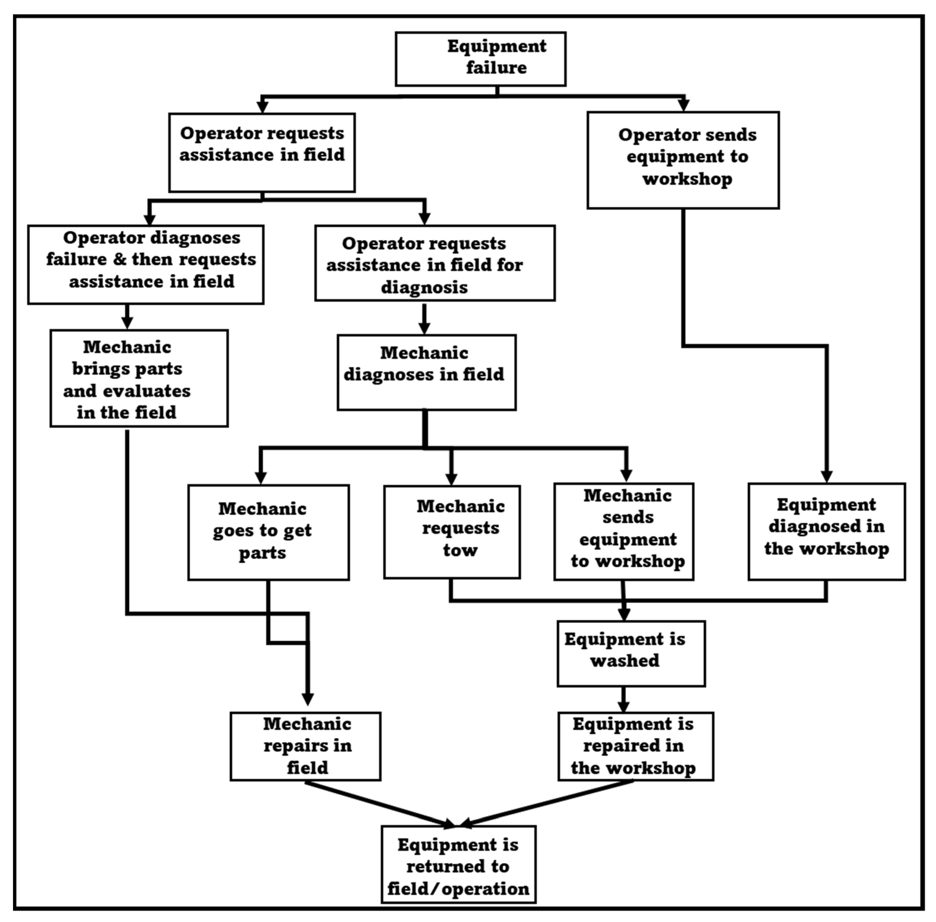
Two maintenance environments are seen in the Disco software process flow—the workshop and the field. All maintenance carried out in the workshop must first go through the “Washing” activity (represented by the “Equipment queued for washing” activity in
Figure 1), which generates a bottleneck. The role of the operator is recognized as the first diagnosis, which is reflected in two key decisions; the first is related to taking the equipment to the workshop or requesting the mechanic to diagnose the equipment in the field. The second is a diagnosis first by the operator and relating the diagnosis to the mechanic or ignoring it (
Figure 1).
Additional activities were detected as part of the process during a conformity analysis with the field experts that could be considered bottlenecks or inefficiencies in the process. Conformance checking techniques compare observed behavior (i.e., event data) with modeled behavior (i.e., process models) to identify deviations. The impact of bottlenecks can be measured in terms of the time added to the maintenance cycle, which entails an opportunity cost defined by the economic value of the material that the equipment does not extract when it is unavailable. The identified activities and bottlenecks identified during conformance checking include the following:
Additional activities:
Mechanic looking for spare parts.
Mechanic travels by work truck.
Mechanic tows the equipment.
Bottlenecks (process delays):
Mechanic leaves to attend to an emergency.
Equipment waiting to be extracted from the field.
Equipment queued for washing.
Mechanic waits for the work truck.
The equipment is disassembled to remove an urgently needed part for another piece of equipment.
The mechanic returns to the workshop to look for a spare part.
Waiting for spare parts
Mechanic waiting for tools.
Five key stages of the process are established and analyzed—diagnosis/initial evaluation, reaction time, failure prioritization, preparation process, effective maintenance, and return to field operations.
5.5.1. Diagnosis/Initial Evaluation
A process filter is first applied, eliminating all instances in which the “Wash” activity is carried out to obtain the instances of field maintenance. This has resulted in 7059 instances (27.5%) of the 25,644 total generated in the 5-year simulation. This value is close to the 30% defined by the field experts as a general rule.
Subsequently, the model is changed to show only the cases that included the “Washing” activity to obtain failures repaired in the workshop, resulting in 18,585 (72.5%) instances. The greater the complexity of these variants is, the higher the variability in the process itself is. Unlike failures repaired in the field, the process to repair in the workshop takes longer, with a mean time to repair (MTTR) of 8.2 h. It is evident that the faults repaired in the field are less acute, repaired faster, and less frequent (
Table 6). Eliminating the bottlenecks in the process can significantly reduce the time to repair and have more people available for critical failures in the workshop or emergencies.
The evaluation of maintenance in the field revealed three inefficiencies in the process. The first was when the operator tells the mechanic that the breakdown can be repaired in the field but misdiagnoses the failure. This occurred in 1062 instances (4.14% of the total), on average, which is 212.4 instances per year. When a misdiagnosis was made, the maintenance process duration increased by 142.2 min, the equivalent of 503 h per year. The second error was when the operator indicated that the failure cannot be repaired in the field, yet it can. This failure occurred in 1669 instances (6.5% of the total) and, on average, 333.8 instances per year. Each time this diagnostic error was generated, the maintenance process duration increased by 112.3 min (625 h per year). The third error in the Diagnosis/Initial Evaluation stage occurred when the operator indicated that it can be repaired in the field but cannot. This failure occurred in 12,579 instances (49% of the total), which was 2515.8 instances per year on average. The maintenance process duration was increased by 16.2 min when such an error was made, resulting in an increase of about 679 h per year.
In the case of workshop maintenance, we analyzed the average time from failure until they reached the “Wash” activity depending on whether the operator requested assistance on-site first (16,335 cases—63.7% of the total cases) or took the equipment directly to the workshop (2250 cases—8.8% of the total cases). In the first instance, it is observed that the average time between the operator carrying out the evaluation in the field and arriving at the workshop for washing was 287.7 min. In contrast, in the second case, it was 73.9 min. This difference occurred because, in 30.6% of the cases in which the operator requested an on-site diagnosis from the mechanic, it was necessary to tow the equipment to the workshop, which had an average duration of 6.7 h. It did not include cases where the equipment was in a condition to be driven directly to the workshop.
It was deduced that 70% of the failures in which the operator requested a field diagnosis did not require towing, and the equipment could have been taken directly to the workshop. If properly diagnosed, this would have generated a saving of 213.7 min in 11,337 cases (44% of the total cases). If the operator had been trained to make a better diagnosis, the availability of the equipment could have increased by 8076 h per year.
5.5.2. Reaction Time
The reaction time of the mechanics was affected by the limited work truck fleet needed to go to the place where the LHD equipment was located. In 7038 instances (27.4% of the total), the mechanics had to wait for a truck, which increased the response time by 44 min per failure. This was equivalent to 1407.6 delays (1032 h) per year.
5.5.3. Failure Prioritization
The third stage of the process is the failure prioritization process. Once an operator requests assistance and a diagnosis of the failure is carried out in the field, it is classified according to whether the equipment needs to be towed and escorted to the workshop (major failure) or can travel to the workshop by itself (minor failure). This classification is relevant when planning which failures to prioritize, given that 4998 instances required towing, with an average transfer time to the workshop of 6.7 h. Comparatively, 11,337 instances did not require towing to the workshop and had an average transfer time of 57 min. In other words, approximately seven units with minor faults are equivalent to one unit with a major failure. This generates a trade-off that must be considered (
Table 7). The effective maintenance time of an acute failure is greater than that of a minor failure. Equipment with an acute failure not removed and taken to a workshop can obstruct haulage ways, preventing its use by other equipment. Therefore, it is important to analyze each case to determine if it is possible to postpone the repair of an acute failure to accelerate the return to the operation of equipment with a minor failure.
5.5.4. Preparation Process
The preparation process begins once the equipment enters the “washing queue” and ends when it reaches the maintenance bay. At this stage, several activities are considered bottlenecks, such as the queue for washing, waiting for tools, equipment disassembly to repair other more critical ones, maintenance breaks to address emergencies, and waiting for spare parts.
Of the instances evaluated, 9268 (36.1% of the total) maintenance tasks were paused to attend to an emergency, which takes an average of 246 min. Instances related to waiting in line to enter the wash were 3709 (14.4% of the total), with an average time of 106.7 min. Additionally, 73 (0.3% of the total) were related to the mechanic waiting for tools for about 13.9 min on average. Cases where the equipment must be disassembled to deliver parts to another piece of equipment with a higher priority to return to operations attributed to 1651 (6.4% of the total cases) instances (an average of 20.1 min). Finally, 5596 (21.8% of the total cases) instances were cases where the team had to wait for a replacement for about 144 min on average. The availability of tools had the least impact compared to other bottlenecks. Notably, the operating losses at this stage totaled 9958 h/year.
5.5.5. Effective Maintenance and Return to Operation
The last stage of the process is the effective maintenance and return to field operation stage. The analysis revealed that 25,644 instances had a MTTR of 6.0 h, with a median of 4.6 h. This indicated that a fair number of minor failures exist that deviate from the meantime to repair. On the other hand, 12,948 (50.5%) of the instances involve equipment waiting an average of 69 min for their return to the field after repair, equivalent to operating losses of 2978 h per year.


