1. Introduction
Air contamination affects the human health, it is considered as one of the major problems in recent days. The ever-growing population and motorization in cities tend to increase the traffic volume which leads to higher gas emissions, etc. [
1]. Air pollution has been a major problem over the past few decades in most developing countries. High levels of air pollutants lead to chronic diseases, such as chronic respiratory diseases, heart failure, bronchitis, etc. People with diabetics, heart and lung disease, and children and elderly people are vulnerable to health effects related to air pollution. Additionally, air pollutants and derivatives can cause many adverse effects related with, e.g., water quality and environment degradation, global climate change, acid deposition, visibility impairment, and plants [
2].
Multivariate Time Series (MTS) is gaining more attention and importance as time series data generation in the Internet of Things (IoT) era advances. A deep learning (DL) architecture is applied for time series forecasting and is still an active research area for different studies. Most researchers focus on applying the single architecture to solve problems in time series forecasting [
3]. Accurate air quality prediction is key to improve the local government’s rapid response [
4]. Particulate Matter (PM) is divided into three major groups, namely: coarse particles (PM
10), fine particles (PM
2.5), and ultrafine particles (PM
0.1). Overall, their sizes vary in source and health effects. In particular, PM
2.5 particles are more active compared to larger pollutants that can spread quickly and remain in the air for a longer time. It also carries substances that affects human health and the surrounding biological environment [
5].
In feature selection, optimization-based methods are used for the intelligent behavior of the spider monkey, which inspired us to develop mathematical models that follow the Fission Fusion Social Structure (FFSS). Effective feature selection techniques help to solve overfitting in classifiers by removing irrelevant features from the extracted ones. Convolutional Neural Network (CNN) based models are applied for feature extraction and classification in various fields of prediction and image processing due to its efficiency [
6,
7,
8,
9,
10,
11,
12,
13]. Accurate air quality prediction models help to control and prevent air pollution and protect residents’ health. Time series based classical statistical models were applied for air quality prediction, they include: Multiple Linear Regression (MLR), and Autoregressive Integrated Moving Average (ARIMA) [
14]. Many researchers focus on time series data for the air quality prediction. Several scientists successfully applied machine learning (ML) models for this purpose. The Support Vector Regression (SVR) is a machine learning technique used to minimize the structural risk based on statistical learning [
15,
16]. Recurrent Neural Network (RNN) models were extensively applied for learning of time series data and Long Short-Term Memory (LSTM) is RNN model to learn long-term temporal dependencies [
17,
18]. Efficient air quality prediction model helps in various fields, including pollution control, sustainability, human health, and government policies. Various models were applied for the air quality prediction process, yet most models face limitations related with the overfitting problem.
The main contributions of this paper are as follows:
The Balanced Spider Monkey Optimization (BSMO) model is proposed in this research for feature selection in air quality prediction. The balancing factor in the BSMO model maintains a tradeoff between the exploration and exploitation that helps to overcome the overfitting and local optima trap.
The Convolutional Neural Network (CNN) model is applied for feature extraction purposes to provide hidden representation of the input dataset. The Bi-directional Long Short-Term Memory (Bi-LSTM) model is used for the prediction process due to its efficiency in handling time series data.
The Balanced Spider Monkey Optimization Bi-directional Long Short-Term Memory (BSMO-BILSTM) model has higher performance than existing methods in air quality prediction. It effectively handles the time series data and delivers less erroneous values.
This paper is organized as follows: an introduction about the air quality prediction is described in
Section 1. The review of recent models of air quality prediction is given in
Section 2, whereas the proposed BSMO-BILSTM model is explained in
Section 3. The simulation setup is given in
Section 4, while obtained results are demonstrated in
Section 5. Finally, the conclusions and future scope of this study are stated in
Section 6.
2. Literature Review
Air quality prediction is important for interdisciplinary air quality research, human health, and sustainable growth, not to mention Quality of Life (QoL), etc. Some of the recent air quality prediction models have been reviewed in this section.
Ragab et al. [
19] applied Exponential Adaptive Gradients (EAG) optimization and 1D-CNN model for prediction process. The 1D-CNN model handled gradients of past model to improve learning rate and convergence. Three years of hourly air pollution were used for training the model. Parameter optimization and model evaluation processes were conducted with a grid search technique. The irrelevant features were selected in the network, and this affected the model performance.
Hashim et al. [
20] performed air quality prediction using weather parameters and hourly air pollution data. Six prediction models, such as Principal Component Regression (PCR), Radial Basis Function (RBFANN), Feed-Forward Neural Network (FFANN), Multiple Linear Regression (MLR), PCA-RBFANN, and PCA-FFANN, were investigated. The developed models had limitations of the overfitting problem due to irrelevant feature selection.
Sun and Liu [
21] applied an ARMA-LSTM model for air quality prediction and a decomposition technique was applied for the data utilization. The vanishing gradient problem and overfitting problem affected the performance of the model once again.
Saufie et al. [
22] applied six wrapper methods, such as genetic algorithm, weight-guided, brute force, stepwise, backward elimination, and forward selection for air quality prediction. Here, Wrapper method has been used for the feature selection. The Multiple Linear Regression (MLR) and Artificial Neural Network (ANN) predictive models were used for the classification process. The model showed that brute-force was the dominant wrapper method and MLR technique provided higher efficiency in the classification. The feature selection technique had local optima and overfitting problems in the classification.
Mao et al. [
23] applied deep learning LSTM-based model for air quality prediction. The multi-layer Bi-LSTM model was applied with optimal time lag to realize sliding prediction based on temporal, meteorological, and PM
2.5 concentrations. The overfitting problem in the classifier affected the model performance.
Zou et al. [
24] applied LSTM based model with spatio-temporal attention mechanism for air quality prediction. A temporal attention technique was used in a decoder to capture air quality dependence. The overfitting problem affected the developed model efficiency in the classification.
Seng et al. [
25] developed a comprehensive prediction technique with multi-index and multi-output based on LSTM. The gaseous pollutant, meteorological, and nearest neighbor stations data were used for prediction of particle concentration. The LSTM based model had considerable performance in air quality prediction on a given dataset. The vanishing gradient and overfitting problem affected the model performance.
Ge et al. [
26] applied a Multi-scale Spatio-Temporal Graph Convolution Network (MST-GCN) for air quality prediction. The MST-GCN model consisted of several spatial-temporal blocks, a fusion block, and a multi-scale block. The extracted features were separated into several groups based on two graphs of spatial correlations and domain categories. The irrelevant features from the selected features caused an overfitting problem in the prediction as well.
Janarthanan et al. [
27] applied LSTM and SVR based model for prediction of air quality in Chennai city. The Grey Level Co-occurrence Matrix (GLCM) was used for extraction of the mean and mean square error, and standard deviation for feature extraction. The DL-based model provided efficient performance in the air quality prediction.
Asgari et al. [
28] developed a parallel air quality prediction system with spatio-temporal data partition techniques, spark efficient environment, ML, resource manager, and Hadoop distributed platform. A distributed random forest technique was used for the evaluation process.
Dun et al. [
29] combined a spatio-temporal correlation and fully connected CNN model for prediction of air quality. Grey relation analysis, PM
2.5 concentrations, and a new calculation method for measuring distance were used during the process. The CNN-based model had an overfitting problem that affected the model performance.
Ma et al. [
30] applied a DL-based model of Graph CNN (GCN) for prediction of air quality. The coordinates of the monitoring points of spatial correlations were considered and Radial Basics Function (RBF) based fusion was conducted. The CNN model had an overfitting problem as well.
According to discussed models, air quality is a major issue that must be resolved in order to prevent or lessen the effects of pollution. For feature selection, Modified Grey Wolf Optimization (MGWO) and Particle Swarm Optimization (PSO) have been used. The state of air will prompt us to take precautions, it may encourage people to carry out their regular activities in less polluted regions. However, it is still difficult to analyze the data and offer better results. Prediction of air pollution is not exempt from the sectors where deep learning technologies bring a significant increase in influence and penetration. In order to effectively predict the air quality, the authors employ sophisticated and advanced approaches. It is crucial to consider external aspects, such as weather conditions, spatial characteristics, and temporal features.
3. Proposed Method
The data were collected from the Central Pollution Control Board (CPCB) for four cities in India. The data were gathered in Bangalore, Chennai, Hyderabad, and Cochin, during a 5 year period between 2016–2022 [
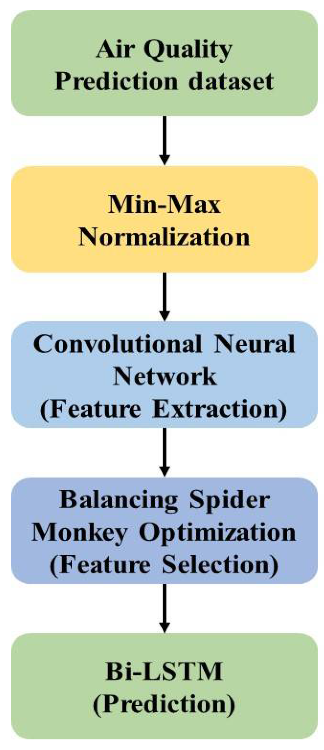
31]. Overall, the process of monitoring pollutants was performed two times a week, during a period of 24 h, which yields 104 observations per year. The normalization was performed using the Min-Max Normalization method that filled the missing values in the dataset. The CNN model was applied to extract the features from the input dataset and provide the hidden representation of features.
The BSMO technique was applied to select the factors from the extracted features for prediction purposes. The BSMO technique applied balancing factors to stabilize the exploration and exploitation in the feature selection which helps to escape from the local optima trap. The overview of the BSMO technique in air quality prediction is shown in
Figure 1.
3.1. Normalization
To maintain the original shape of the image, min-max normalization provided relationships among the original data values. This constrained range came at the expense of smaller standard deviations that supported to reduce the impact of outliers. The Min-Max Normalization technique was applied to reduce the difference between respective values in the dataset. The formula for Min−Max Normalization is given in Equations (1) and (2):
where the minimum feature range of input data
is
, and the maximum feature range is
.
3.2. CNN Based Feature Extraction
The CNN models consist of neurons organized in a layer to learn hierarchical representations similar to the typical neural network type [
32,
33,
34]. Weights and biases are used to connect neurons. The input layer takes the initial data and processes them into a final layer that provides the prediction of the model. Input feature space transforms hidden layers to match its output. Generally, CNNs are applied with a minimum of one convolutional layer to exploit patterns. The architecture of the CNN is shown in
Figure 2.
CNN are widely used in medical research, natural language processing, and other fields. Researchers found that CNN models have unique advantages for processing of input data and provide hidden representation. This study applies 1D time series data as input and air quality index of the next movement as an output to train a 1D-CNN model for prediction of air quality at the next step.
The input time series data is denoted as
with a length of
. The air quality index of the corresponding feature of output is denoted as
with a vector length of 10. The 1D-CNN learning goal is a non-linear mapping between the input factor and air quality index output for next time period, as described in Equation (3):
where a complex non-linear mapping of input and output is denoted as
. For better representation of complex mapping relationships, the time series prediction problem is converted to MSE. The MSE finds the minimum set to reduce differences between relationship fitted to mapping function
and real relationship, as provided in Equation (4):
Calibrate output and output differences are reduced using this process. Neural network processing is used to adjust the parameters.
The multi-layer CNN model is used in this study and consists of a total number of
layers. The input
is the upper layer output for
convolutional layer and
layer output is given in Equation (5):
where convolution kernel weight is denoted as
and non-linear activation function is denoted as
. After the convolution process, offset
is added for a better non-linear fitting. The Rectified Linear Unit (ReLU) function is applied as an activation function for the
layer of a convolutional layer. The activation function is used as a layer of sigmoid function for the fully connected layer of the
layer. The non-linear relationship of input and output is denoted in Equation (6):
The last layer provides the output of the CNN that consists of many features and back propagation is performed to reduce the error between calibration output and output. This helps to adjust the optimization parameters to reduce differences based on mean square error for minimization. The input data are convolved, pooled, fully connected, and multi-classified for a 1D-CNN, and, finally, features are extracted for the prediction process. The fully connected layer is shown in
Figure 3.
It consists of four parts: a fully connected layer, 1D pooling layer, 1D convolutional layer, and 1D-input layer. The pooled layer and convolution kernels are different from a two-dimensional CNN structure that also have a one-dimensional pooled layer structure.
1D-CNN convolution process: In a 1D CNN, the first layer of convolution is considered as an operational relationship between input data
and weight vector
. The size of a weight vector is
and the convolution kernel size is also
. Specifically, each element of air quality concentration for that instance and air quality index period of output vector is denoted as
. Each
sequence of convolution kernel size
with length of input vector is used to provide first layer output. The air quality concentration value is denoted as
at input of each moment, which is included in the convolution operation. The step size is set as 1, and the convolution formula is given in Equation (7):
1D-Convolution Layer: The one-dimensional vector is applied for 1D convolution layer; therefore, convolution kernel is set as one-dimensional. A 1D convolution process is used to provide the convolution process, more specifically, for an input length of 7, a kernel size of 5, and a convolution step of one.
1D-Convolution pooling layer: The 1D-CNN fully exerts the neural network due to existence of a pooling layer for feature extraction. The 1D-CNN training speed is inherently higher than other neural networks.
3.3. Balanced Spider Monkey Optimization
The spider monkey’s intelligent behavior is inspired to develop SMO mathematical models that follow the FFSS [
35,
36,
37]. Monkeys distribute from larger to smaller groups and smaller to larger for foraging based on FFSS. The BSMO steps are given as follows:
Initially, spider monkeys are present as 40–50 individuals in a group. Every group has a leader that makes decision for exploration of food, and this is a global leader of that group.
If food quality is insignificant, smaller sub-groups are created by the global leader. Each sub-group contains 3 to 8 members independently foraging, and each subgroup is led by a local leader.
For each sub-group, food search decision is selected by a local leader.
Communication of defensive boundaries and social bonds maintained by group members is conducted, and a unique sound is used by other members in that group.
The SMO foraging behavior of mathematical models is used for optimization problems and consist of six different phases. The SMO applies a 1D vector to denote a spider monkey and
spider monkey populations are randomly generated by SMO. Consider
, which provides
with the dimension of
, the individual. Each
of SMO is used to initialize as described in Equation (8):
where lower and upper bounds of
in
direction are
and
, random number in the range of [0, 1] is denoted as
. The six phases of SMO are discussed as follows.
3.3.1. Local Leader Phase (LLP)
A new position individual is attained in this phase on basic knowledge of a local leader and group individuals, as described in Equation (9). The fitness value is used to decide a particular solution regarding quality. The highest fitness solution is selected for the next iteration:
where
is the direction of a local group leader position denoted as
and
, and
spider monkey is selected from
group, respectively. In order to maintain perturbation of present location, perturbation rate or probability
is used.
3.3.2. Global Leader Phase (GLP)
Global leader information is used to update individual spider monkey positions and group members, as denoted in Equation (10):
where global leader of
direction is denoted as
. The probability
is used to select particular dimension for
update and fitness value is calculated for each individual, according to Equation (11):
The better solution similar to LLP are newly generated position and spider monkey’s old position is used for further processing.
3.3.3. Global Leader Learning (GLL) Phase
Global leader overall best fitness is provided in this phase and position change of the global leader is noted.
3.3.4. Local Leader Learning (LLL) Phase
Local leader is the best fitness position in the group. If the previous position of a local leader remains the same, then, similar to the GLL phase, local limit counter is updated with one.
3.3.5. Local Leader Decision (LLD) Phase
If a local limit counter of a local leader reaches to threshold count, then group members are reinitialized according to Equation (12):
3.3.6. Global Leader Decision (GLD) Phase
If a leader position was not updated for the applied iterations, then the global leader creates small sub-groups. The GLD of each group’s local leaders are selected using the LLL phase. If the position is not updated for a time threshold value, then the global leader merges smaller groups to a single group. The SMO process of FFS structure is processed in this phase.
The balanced factor is proposed to provide a new global weighting coefficient
to control past classes importance using Equation (13):
where weighting coefficient
is a real number, and the set of previous encountered classes denoted as
, usually between 0 and 1. The coefficient
expression is not changed for new classes, and the training set
number of images for old classes is multiplied using weighting coefficient
. The flow chart of BSMO method is shown in
Figure 4.
3.4. Bi-LSTM for Classification
The RNN based models are effective for time series applications, and this model has capacity to learn temporal dependencies. An RNN-based model has the possibility to learn current data based on previous data. RNN learn long term dependencies to solve one of RNN variants. The LSTM model, shown in
Figure 5, is an improved version of the RNN and LSTM, and consists of memory cell or hidden layers to learn the long-term dependencies. Three gates, such as forget, input, and output, were used in memory cells to store temporal state of a network [
38,
39,
40]. Network rest output and input control of a control memory cell is based on the output and input gate. Additionally, the forget gate in a network helps to pass high weight information to next neurons and discard the remaining ones. The activation function is used to determine the weight values for information and the high weight value of information is forwarded to the following neurons.
The input and output sequence are mapped using a LSTM network, i.e.,
, calculated according to Equations (14)–(17):
where weights and biases are represented using
,
,
, and
, and
,
,
, and
for memory cells and three gates, respectively. The prior hidden layer unit is used to represent
and three gates’ weights is added element wise. After processing described in Equation (13), a current memory cell unit is updated using
. The previous cell unit element wise is multiplied, and the output of the hidden unit is processed as described in Equation (14). Three gates are added with non-linearity in form of
and sigmoid activation function, as in Equations (14)–(17). The current time step is denoted as
and previous time step is denoted as
.
LSTM cell can work on previous content and not on future ones. The bi-directional recurrent neural network is shown in
Figure 6. The input sequence is denoted as
, Bi-LSTM forward direction is denoted as
, and backward direction as
. The final cell output
is formed using
and
, the output final sequence is denoted as
.
4. Simulation Setup
Dataset: The majority of Indian cities continue to fall short of both national and global PM10 air quality targets. Pollution from respirable particulate matter continues to be a major problem for India. Some cities demonstrated far more improvement than others, despite the overall non-attainment, establishing the execution of a comprehensive plan for the prevention, control, and reduction of air pollution. The SO2, NOx, and PM10 are the major air pollutants that India’s Central Pollution Control Board currently regularly monitors. Currently, these actions are realized regularly at 308 operating stations in 115 cities and towns throughout 25 states and 4 Indian union territories. Along with the monitoring of air quality, meteorological parameters, such as relative humidity, temperature, relative wind speed, location, and direction, are also included. The monitoring of these pollutants is done twice a week during a 24 h period, yielding 104 observations per year. The parameters considered for this research were: SO2, NOx, and PM2.5. The data were collected in four cities in India, namely Bangalore, Chennai, Hyderabad, and Cochin, between 2016–2022 from the CPCB.
Metrics: As this model is a time series prediction, the error values such as MSE, RMSE, and MAE, have been calculated and compared with existing technique. The metrics equations are given as follows in Equations (18)–(20):
where
denotes the number of data points,
represents observed values, and
relates to predicted values.
where
denotes the prediction value,
represents the true value, and
relates to the total number of data points.
System Requirement: The BSMO technique was tested on a desktop PC stand with an Intel i9 processor, 128 GB of RAM, a 22 GB graphics card, and Windows 10 as the serving OS. The Python 3.7 tool was used to implement the proposed model.
Parameter settings: For the CNN model, the learning rate was set to 0.001, and number of epochs was equal to 30. For the BSMO technique, the population was denoted as 50, whereas the number of iterations was fixed to 50, and the balancing factor of threshold value was set to 0.5. Bi-LSTM consists of 3 input/output layers and two hidden layers with similar output of opposite direction, which has 32 neurons. The output layer is exploited with previous and future information with this architecture. The Bi-LSTM model was applied with 30 epochs, with early stopping, 0.01 learning rate, and 0.1 dropout rate.
5. Results
In the result analysis, the proposed air quality prediction model helps to solve overfitting issues by removing irrelevant features in extracted features.
Figure 7 displays the Mean Standard Error (MSE) value of the Bi-LSTM model as it predicted the air quality index [
19,
27] for several epochs.
The MSE value of the Bi-LSTM model was reduced up to 26 epochs and started to increase due to the overfitting problem. The early stopping technique stops the model at the 26th epoch and prevents overfitting in the model. Various DL techniques were applied for the feature extraction process and performance measurements. Their results are shown in
Table 1.
The deep learning techniques provide the hidden representation of features in the air quality prediction. DL provides features for the classifier for better representation of input data. The Bi-LSTM and BSMO model are commonly applied for feature extraction techniques for fair comparison. The CNN model has lower error value compared to other DL models, because other models have a higher number of convolution, and pooling layers that cause the overfitting problem in the classification. The CNN feature extraction with the BSMO and BILSTM obtained 0.318 MSE, 0.564 RMSE, and 0.224 MAE, whereas the existing ResNet reached 0.348 MSE, 0.590 RMSE, and 0.625 MAE, respectively. The BSMO technique has been compared with existing feature selection techniques in terms of error measure. Their results are shown in
Table 2.
The BSMO technique achieves higher performance than existing feature selection methods. The BSMO technique has a balancing factor that maintains a tradeoff between exploration and exploitation. This process helps to overcome the local optima trap and reduces overfitting in the classification process. The existing feature selection techniques have limitations of the local optima trap and lower convergences in the feature selection. The BSMO-BILSTM technique obtained 0.318 MSE, 0.564 RMSE, and 0.224 MAE, whereas the WOA method reached 0.783 MSE, 0.885 RMSE, and 0.189 MAE, respectively, in air quality prediction. The BSMO-BILSTM model has been compared with various classifiers for air quality prediction. Their results are shown in
Table 3. The classifiers, such as Support Vector Machine (SVM), Random Forest (RF), and K Nearest Neighbors (KNN), were compared with the proposed BSMO-BILSTM.
The KNN model is sensitive to the outlier, whereas the RF model has an overfitting problem and SVM has an imbalance data problem. The LSTM model has an overfitting and vanishing gradient problem that affects performance. The BSMO technique selects the features based on the balancing factor in order to avoid overfitting, and increase learning performance. The BSMO-BILSTM model has higher performance due to an effective feature selection process. The BSMO-BILSTM obtained 0.318 MSE, 0.564 RMSE, and 0.224 MAE, whereas the KNN reached 0.816 MSE, 0.903 RMSE, and 0.894 MAE, respectively. The BSMO-BILSTM model has been compared with existing methods in air quality prediction. Their results are shown in
Table 4.
From
Table 4, The BSMO-BILSTM model has a lower error value than the existing models in air quality prediction. The BSMO method offers an advantage of applying balancing factor to maintain the exploration–exploitation feature selection that helps to overcome the local optima trap and overfitting problem. The existing Attention LSTM [
24] method suffers from the vanishing gradient problem, BI-LSTM [
23] has lower efficiency feature representation, whereas ARIMA-LSTM [
21] and EAG-CNN [
19] have an overfitting problem. The BSMO-BILSTM model obtained 0.318 MSE, 0.564 RMSE, and 0.224 MAE, whereas the Attention LSTM [
24] reached 0.699 MSE, 0.836 RMSE, and 0.892 MAE, respectively.
Discussion
For the air quality prediction procedure, a variety of models were used, however the majority of them had issues with overfitting. By deleting pointless features from extracted features, the efficient feature selection technique, known as Balance Spider Monkey Optimization (BSMO), helps to address overfitting in classifiers.
In this collected dataset (two times a week during a 24 h time period), these pollutants were monitored, giving 104 observations annually. The variables considered for this study were: SO2, NOx, and PM2.5. The Central Pollution Control Board provided the statistics, which were gathered in four Indian cities between 2016 and 2022, namely Bangalore, Chennai, Hyderabad, and Cochin. The suggested BSMO-BILSTM was compared to classifiers including: Support Vector Machine (SVM), Random Forest (RF), and K Nearest Neighbors (KNN). According to our findings, the Attention LSTM model achieved 0.699 MSE, 0.836 RMSE, and 0.892 MAE, whereas the proposed BSMO-BILSTM model attained 0.318 MSE, 0.564 RMSE, and 0.224 MAE, respectively.
6. Conclusions
Currently, air quality predictions have become a crucial task, particularly in developing nations. The deep learning-based prediction technologies have been shown to be more effective than conventional methods for researching these contemporary threats. DL algorithms are capable of handling difficult analyses required to perform accurate and reliable predictions from such large environmental data. Yet, DL techniques applied in air quality prediction have an overfitting problem due to irrelevant feature selection. This study proposes the BMSO-BILSTM model to select relevant features based on the balancing factor in order to overcome this problem. The Balanced Spider Monkey Optimization (BMSO) method maintains exploration and exploitation to select relevant features for further classification. The BMSO-BILSTM model obtains higher performance in air quality prediction in case of data from four cities analyzed in this paper. The CNN model was used to provide a hidden representation of the input dataset and the BILSTM model enables efficient classification. The BSMO-BILSTM model obtained 0.318 MSE, 0.564 RMSE, and 0.224 MAE, whereas the Attention LSTM reached 0.699 MSE, 0.836 RMSE, and 0.892 MAE, respectively.
Air quality prediction is extremely useful for governments to control pollution, including various human health and sustainability issues. The findings of this investigation can be further enhanced. In future studies, it could include, e.g., a hyper parameter optimization in the Bi-LSTM model to reduce the error of prediction. Results of this study may support various governmental and non-government institutions focused on maintaining a stable and healthy development of both the local community and provinces or states. It could surely help in sustaining a stable advancement and high quality of life of modern-day societies while keeping pollution at the lowest possible level. Still, the process of analyzing data and providing better solutions remains a challenge. In order to analyze large amounts of data more effectively and efficiently, make the invisible visible, and extract the hidden data which is crucial to use effective methodologies and procedures. Therefore, in the future, this research will be further extended by analyzing the air quality prediction in some other regions with different methodologies to improve the statistical measures.


 and
and 


