
Optimal Design of an Eco-Friendly Transportation Network under Uncertain Parameters

 ,
, 
 ,
,  ,
, 
Abstract
:1. Introduction
1.1. Research Motivation
1.2. Research Objectives
- Different types of MADM approaches, viz., MAUT, ELECTRE, TOPSIS, and Exp-TOPSIS have been stated, step by step.
- Exp-TOPSIS has been proposed which is the expansion of the TOPSIS method.
- A case study of carbon emissions is shown with the use of some practical data in the form of zigzag uncertain variables.
- An STP has been proposed to show the application of MADM methods.
- All the MADM methods have been utilized to present the ranking with different weights of attributes and also with the same weights of attributes.
- From those rankings, the best five have been taken, and accordingly, these are used to solve the proposed STP with the use of Lingo 13.0 iterative software.
2. Review of the Relevant Literature
- In this paper, taking uncertainty into account, four different MADM techniques have been discussed and MAUT is one of them. As the preferences are used as the input in this technique, these preferences should be precise [42,43]. This study incorporates this method to solve a sustainable STP model since it can be applied to many fields, namely, agriculture, energy management, finance, and others. Section 4.1 presents detailed explanations of this process.
- The ELECTRE is one of the techniques which can be applied, which takes uncertainty and vagueness into account, and is presented in [44]. The process and its results can be difficult to explain simply; upping the rankings means that the strengths and weaknesses of the alternatives are not directly identified. This study uses this method in the solution process of the proposed mathematical model, and the related detailed explanations are available in Section 4.2.
- Because of the simple methodological aspect of the TOPSIS, this study considers this method as well [45,46]. The correlation of attributes sometimes makes it difficult to keep the consistency of judgment in many MCDM methods, whereas TOPSIS does not focus on the correlation between attributes. It has applications in many areas such as logistics and supply chain management, engineering, production systems, sales and marketing, environment, human resource management, and water resources. The detailed utilization of TOPSIS in solving the proposed model is available in Section 4.3.
- Finally, the Exp-TOPSIS, a modified version of the TOPSIS, was developed with a change in the technique of giving preferences to orders by similarity to ideal solutions based on the exponential function. As the exponential function indicates the rate of change in expression to the most recent one, it is giving them more realistic and accurate multi-criteria-based decisions. Thus, it is proposed and used hereby in this research article to solve a real-life-based case study designated to a supply chain-oriented optimization problem. Section 4.4 gives detailed explanations of this method.
3. Basic Concepts of Uncertainty Theory
3.1. Definition
3.2. Theorem
4. Decision-Making Process
4.1. Multi-Attribute Utility Theory
4.2. ELECTRE Method
4.3. TOPSIS Method
4.4. Proposed Exp-TOPSIS
5. Case Study: A Carbon Emission Solid Transportation Problem
5.1. Case Study Related to Carbon Emissions
5.2. Case Study Related to Solid Transportation Problem
5.3. Materials and Methods
- The parameters of the problem are defined using the analysis made on the past data and experienced experts’ opinions.
- The transportation problem has involved the transportation of goods from their source point to the demand point using different vehicles and it is an unbalanced problem.
- The problem is focused to make an analysis to choose the best factors that optimize the total carbon emissions from the vehicles.
| i | Indices to the distribution center. |
| j | Indices to the demand point. |
| k | Indices to the vehicle type used. |
| l | Indices to the different carbon emission factors. |
| l1 | Set of emission factors proportional to the distance traveled by the vehicle. |
| l2 | Set of emission factors proportional to the load or fuel type used in the vehicle. |
| Uncertain emission rate for the vehicle k on the route (i, j) considering the l-th factor. | |
| Uncertain extra per unit carbon emissions for the k-th vehicle due to the l-th factor. | |
| dij | Distance between the i-th source point and the j-th demand point. |
| Uncertain emissions at the per unit rate due to the vehicle’s load. | |
| Uncertain emissions at the per unit rate due to the vehicle’s fuel type. | |
| Efficiency based on per unit uncertain emissions caused by the l-th factor. | |
| Ok | Driver efficiency, driving the k-th vehicle. |
| Ek | Per unit emissions for the vehicle type used in transportation. |
| Uncertain available amount of transported items at the i-th source point. | |
| Uncertain demand from the j-th demand point. | |
| Define the uncertain capacity of the k-th vehicle. |
5.4. Model Description
6. Numerical Analysis
6.1. Input Tables
6.2. Decision-Making Process Using MADM
6.2.1. Rank Obtained Using MAUT
6.2.2. Rank Obtained Using ELETRE Method
6.2.3. Rank Obtained with TOPSIS Method
6.2.4. Rank Evaluation Using Proposed Exp-TOPSIS
7. Results and Discussion
7.1. Convergence Test of Proposed Exp-TOPSIS
7.2. Advantage of the Proposed Method
7.3. Managerial Insights
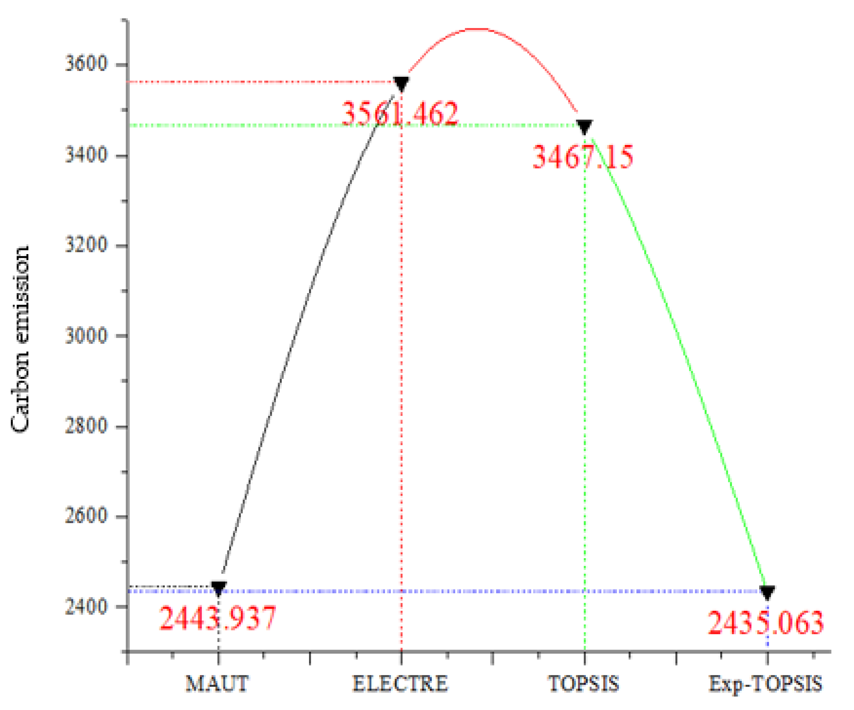
- Same weights mean giving the same preferences to all the attributes, which defines the uniformity and unbiasedness for a fair comparison to the performance of four MADM processes and it is observed that the proposed MADM process gives the best minimal carbon emission. Hence, a decision-maker can choose the proposed method not only to optimize carbon emissions but other optimization problems such as the optimization of cost, time, profit, social economic disruption, etc.
- The Exp-TOPSIS is based on the exponential function, and it always gives the rate of the change in expression that is related to a particular decision-making attribute. Thus, it is suggested to use the proposed method when the case of decision-making is sensitive. The results obtained for the proposed model can be considered as evidence.
- The proposed mathematical model is an optimization model originating from a linear programming problem; thus, it opens several ideas to use in a different situation where the objective is to optimize with respect to the given constraints. For example, traveling means sales problems, job assignment problems, cold supply chain-based inventory problems, vehicle routing problems, facility locations problems, etc., considering uncertainty.
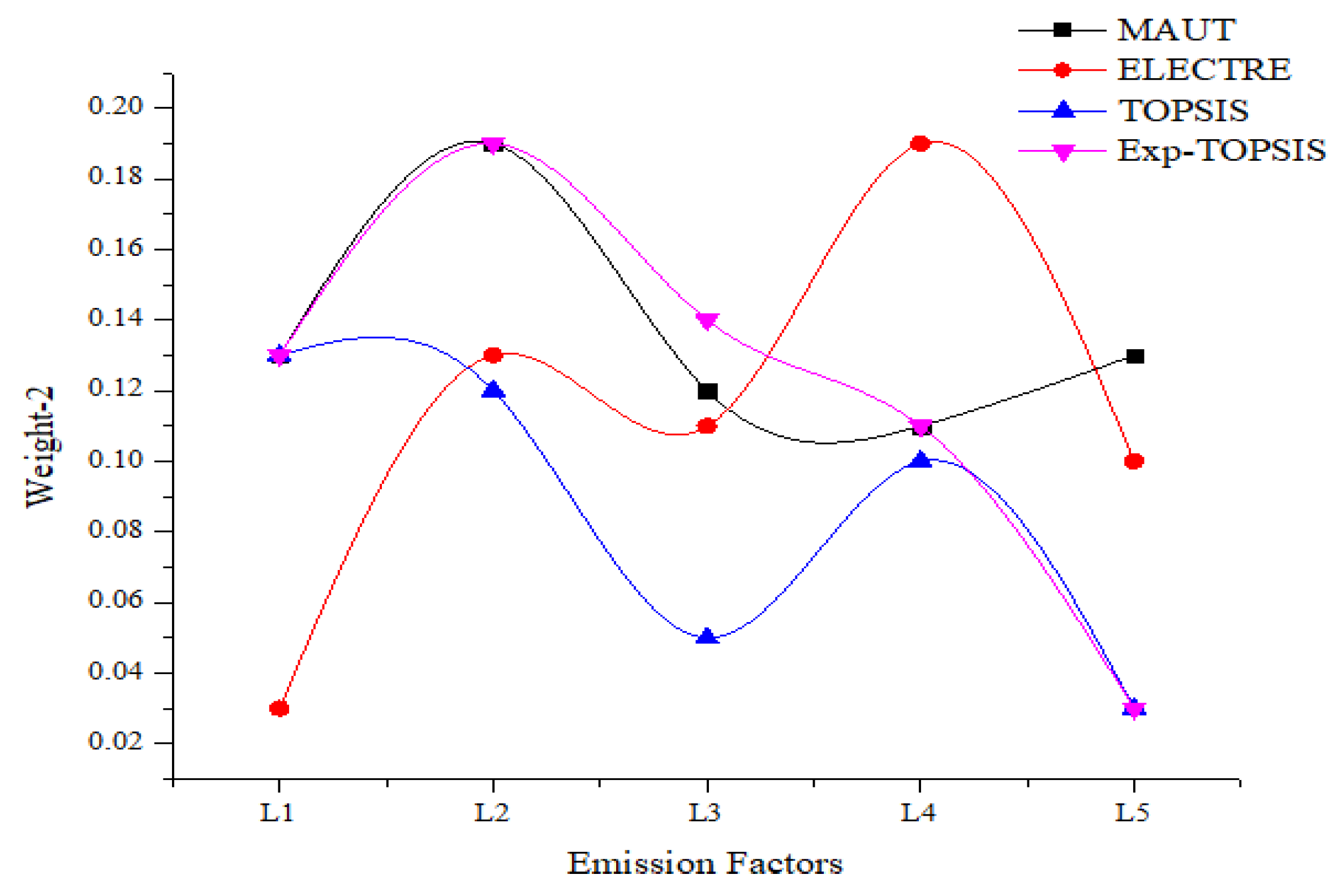
- This study also analyzed the impact of choosing different weights in the objective value and this is observed in Table 10, and also in Figure 5, which represents the same with a comparison to the case if we choose the same weights. Here, for the different weights, ELECTRE gives the optimal emissions, as this process consists of elimination and choice based on the expression of reality, rather than the rate of change in expression. This process is okay sometimes when the expression is available in reality but it is very rare and of high risk; thus, our proposed process would be a better one from a reliability point of view.
8. Conclusions and Future Scope
- Four MADM processes, MAUT, ELECTRE, TOPSIS, and Exp-TOPSIS, are discussed in a step-by-step manner.
- A novel method of Exp-TOPSIS is proposed, which is the extension of the TOPSIS method.
- A case study of carbon emissions is shown with the use of some practical data in the form of the zigzag uncertain variable.
- A mathematical model for an STP is formulated to show the use of MADM methods.
- All the MADM methods are utilized to present the ranking with the different weights of attributes and the same weights of attributes.
- The proposed STP is solved using Lingo 13.0 iterative software from those five best rankings.
- The managerial insights have been drawn to analyze the results at the end.
Author Contributions
Funding
Institutional Review Board Statement
Informed Consent Statement
Data Availability Statement
Acknowledgments
Conflicts of Interest
References
- IEA. CO2 Emissions from Fuel Combustion Highlights; IEA: Paris, France, 2015; 139p, Available online: https://iea.blob.core.windows.net/assets/eb3b2e8d-28e0-47fd-a8ba-160f7ed42bc3/CO2_Emissions_from_Fuel_Combustion_2019_Highlights.pdf (accessed on 19 March 2023).
- Choudhary, A.; Sarkar, S.; Settur, S.; Tiwari, M. A carbon market sensitive optimization model for integrated forward–reverse logistics. Int. J. Prod. Econ. 2015, 164, 433–444. [Google Scholar] [CrossRef]
- Seo, J.; Park, J.; Oh, Y.; Park, S. Estimation of Total Transport CO2 Emissions Generated by Medium- and Heavy-Duty Vehicles (MHDVs) in a Sector of Korea. Energies 2016, 9, 638. [Google Scholar] [CrossRef] [Green Version]
- Liu, B. Uncertainty Theory; Springer: Berlin/Heidelberg, Germany, 2007; pp. 205–234. [Google Scholar]
- Liu, Y.; Ha, M. Expected Value of Function of Uncertain Variables. J. Uncertain Syst. 2010, 4, 181–186. [Google Scholar]
- Liu, B.; Liu, B. Theory and Practice of Uncertain Programming; Springer: Berlin/Heidelberg, Germany, 2009. [Google Scholar]
- Liu, B.; Chen, X. Uncertain Multiobjective Programming and Uncertain Goal Programming. J. Uncertain. Anal. Appl. 2015, 3, 73. [Google Scholar] [CrossRef] [Green Version]
- Cui, Q.; Sheng, Y. Uncertain programming model for solid transportation problem. Int. Inf. Inst. Inf. 2013, 16, 1207. [Google Scholar]
- Sheng, Y.; Yao, K. A transportation model with uncertain costs and demands. Information 2012, 15, 3179–3185. [Google Scholar]
- Alam, S.T.; Ahmed, S.; Ali, S.M.; Sarker, S.; Kabir, G.; Ul-Islam, A. Challenges to COVID-19 vaccine supply chain: Implications for sustainable development goals. Int. J. Prod. Econ. 2021, 239, 108193. [Google Scholar] [CrossRef]
- Rosanty, E.S.; Dahlan, H.M.; Che Hussin, A.R. Multi-criteria decision making for group decision support system. In Proceedings of the International Conference on Information Retrieval and Knowledge Management, CAMP’12, Kuala Lumpur, Malaysia, 13–15 March 2012; pp. 105–109. [Google Scholar]
- Ilgin, M.A.; Gupta, S.M.; Battaïa, O. Use of MCDM techniques in environmentally conscious manufacturing and product recovery: State of the art. J. Manuf. Syst. 2015, 37, 746–758. [Google Scholar] [CrossRef] [Green Version]
- Abbasbandy, S.; Asady, B. Ranking of fuzzy numbers by sign distance. Inf. Sci. 2006, 176, 2405–2416. [Google Scholar] [CrossRef]
- Abbasbandy, S.; Hajjari, T. A new approach for ranking of trapezoidal fuzzy numbers. Comput. Math. Appl. 2009, 57, 413–419. [Google Scholar] [CrossRef] [Green Version]
- Zopounidis, C.; Doumpos, M. Multi-criteria decision aid in financial decision making: Methodologies and literature review. J. Multi-Criteria Decis. Anal. 2002, 11, 167–186. [Google Scholar] [CrossRef]
- Anand, M.D.; Selvaraj, T.; Kumanan, S.; Johnny, M.A. Application of multicriteria decision making for selection of robotic system using fuzzy analytic hierarchy process. Int. J. Manag. Decis. Mak. 2008, 9, 75. [Google Scholar] [CrossRef]
- Carlsson, C.; Fullér, R. Fuzzy multiple criteria decision making: Recent developments. Fuzzy Sets Syst. 1996, 78, 139–153. [Google Scholar] [CrossRef] [Green Version]
- Kundu, P.; Kar, S.; Maiti, M. A fuzzy MCDM method and an application to solid transportation problem with mode preference. Soft Comput. 2013, 18, 1853–1864. [Google Scholar] [CrossRef]
- Samanta, S.; Jana, D.K. A multi-item transportation problem with mode of transportation preference by MCDM method in interval type-2 fuzzy environment. Neural Comput. Appl. 2019, 31, 605–617. [Google Scholar] [CrossRef]
- Ribeiro, R.A. Fuzzy multiple attribute decision making: A review and new preference elicitation techniques. Fuzzy Sets Syst. 1996, 78, 155–181. [Google Scholar] [CrossRef]
- Triantaphyllou, E.; Chi-Tun, L. Development and evaluation of five fuzzy multiattribute decision-making methods. Int. J. Approx. Reason. 1996, 14, 281–310. [Google Scholar] [CrossRef] [Green Version]
- Abdullah, L. Fuzzy Multi Criteria Decision Making and its Applications: A Brief Review of Category. Procedia Soc. Behav. Sci. 2013, 97, 131–136. [Google Scholar] [CrossRef] [Green Version]
- Güzel, N.; Alp, S.; Geçici, E. Solving solid transportation problems under uncertain environment using goal programming. J. Ind. Eng. 2022, 33, 130–144. [Google Scholar]
- Roy, S.K.; Midya, S. Multi-objective fixed-charge solid transportation problem with product blending under intuitionistic fuzzy environment. Appl. Intell. 2019, 49, 3524–3538. [Google Scholar] [CrossRef]
- French, S.; Roy, B. Multicriteria Methodology for Decision Aiding. J. Oper. Res. Soc. 1997, 48, 1257. [Google Scholar] [CrossRef]
- Roy, B. The Outranking Approach and the Foundations of Electre Methods, Readings in Multiple Criteria Decision Aid; Springer: Berlin/Heidelberg, Germany, 1990; pp. 155–183. [Google Scholar] [CrossRef]
- Wang, Y.-J.; Lee, H.-S. Generalizing TOPSIS for fuzzy multiple-criteria group decision-making. Comput. Math. Appl. 2007, 53, 1762–1772. [Google Scholar] [CrossRef] [Green Version]
- Haley, K.B. New Methods in Mathematical Programming—The Solid Transportation Problem. Oper. Res. 1962, 10, 448–463. [Google Scholar] [CrossRef]
- Das, A.; Bera, U.K.; Das, B. A solid transportation problem with mixed constraint in different environment. J. Appl. Anal. Comput. 2016, 6, 179–195. [Google Scholar] [CrossRef]
- Kundu, P.; Kar, S.; Maiti, M. Multi-objective multi-item solid transportation problem in fuzzy environment. Appl. Math. Model. 2013, 37, 2028–2038. [Google Scholar] [CrossRef]
- Jana, S.H.; Das, B.; Panigrahi, G.; Maiti, M. Some special fixed charge solid transportation problems of substitute and breakable items in crisp and fuzzy environments. Comput. Ind. Eng. 2017, 111, 272–281. [Google Scholar] [CrossRef]
- Sinha, B.; Das, A.; Bera, U.K. Profit Maximization Solid Transportation Problem with Trapezoidal Interval Type-2 Fuzzy Numbers. Int. J. Appl. Comput. Math. 2015, 2, 41–56. [Google Scholar] [CrossRef] [Green Version]
- Das, A.; Bera, U.K.; Maiti, M. A Profit Maximizing Solid Transportation Model under a Rough Interval Approach. IEEE Trans. Fuzzy Syst. 2016, 25, 485–498. [Google Scholar] [CrossRef]
- Das, A.; Bera, U.K.; Maiti, M. Defuzzification and application of trapezoidal type-2 fuzzy variables to green solid transportation problem. Soft Comput. 2018, 22, 2275–2297. [Google Scholar] [CrossRef]
- Soysal, M.; Bloemhof-Ruwaard, J.M.; Van Der Vorst, J.G.A.J. Modelling food logistics networks with emission considerations: The case of an international beef supply chain. Int. J. Prod. Econ. 2014, 152, 57–70. [Google Scholar] [CrossRef]
- Pan, S.; Ballot, E.; Fontane, F. The reduction of greenhouse gas emissions from freight transport by pooling supply chains. Int. J. Prod. Econ. 2013, 143, 86–94. [Google Scholar] [CrossRef]
- Watkiss, P. The Social Cost of Carbon; DEFRA: London, UK, 2005.
- Yang, H.; Huang, H.-J. The multi-class, multi-criteria traffic network equilibrium and systems optimum problem. Transp. Res. Part B Methodol. 2004, 38, 1–15. [Google Scholar] [CrossRef]
- Tzeng, G.-H.; Lin, C.-W.; Opricovic, S. Multi-criteria analysis of alternative-fuel buses for public transportation. Energy Policy 2005, 33, 1373–1383. [Google Scholar] [CrossRef]
- Yeh, C.H.; Chang, Y.H. Modeling subjective evaluation for fuzzy group multi-criteria decision making. Eur. J. Oper. Res. 2009, 194, 464–473. [Google Scholar] [CrossRef]
- Hwang, C.-L.; Yoon, K. Methods for Multiple Attribute Decision Making, Multiple Attribute Decision Making; Springer: Berlin/Heidelberg, Germany, 1981; pp. 58–191. [Google Scholar]
- Bukhsh, Z.A.; Stipanovic, I.; Doree, A.G. Multi-year maintenance planning framework using multi-attribute utility theory and genetic algorithms. Eur. Transp. Res. Rev. 2020, 12, 1–13. [Google Scholar] [CrossRef]
- Taufik, I.; Alam, C.N.; Mustofa, Z.; Rusdiana, A.; Uriawan, W. Implementation of Multi-Attribute Utility Theory (MAUT) method for selecting diplomats. IOP Conf. Ser. Mater. Sci. Eng. 2021, 1098, 032055. [Google Scholar] [CrossRef]
- Sarwar, M.; Akram, M.; Liu, P. An integrated rough ELECTRE II approach for risk evaluation and effects analysis in automatic manufacturing process. Artif. Intell. Rev. 2021, 54, 4449–4481. [Google Scholar] [CrossRef]
- Arya, S.; Chitranshi, M.; Singh, Y. Analysing Distance Measures in Topsis: A Python-Based Tool. In Proceedings of International Conference on Scientific and Natural Computing; Springer: Berlin/Heidelberg, Germany, 2021; pp. 275–292. [Google Scholar]
- Kumar, A.; Kothari, R.; Sahu, S.K.; Kundalwal, S.I. Selection of phase-change material for thermal management of electronic devices using multi-attribute decision-making technique. Int. J. Energy Res. 2021, 45, 2023–2042. [Google Scholar] [CrossRef]
- Liu, B. Why is there a need for uncertainty theory? J. Uncertain Syst. 2012, 6, 3–10. [Google Scholar]


| i/k | 1 | 2 | 3 | 4 | 5 | j | |
|---|---|---|---|---|---|---|---|
| for fuel type | 1 | (1.2, 1.3, 1.4) (1.1, 1.2, 1.3) (1.5, 1.7, 1.8) | (1.3, 1.4, 1.5) (1.4, 1.6, 1.7) (1.4, 1.6, 1.8) | (1.4, 1.5, 1.6) (1.8, 1.9, 2) (1.2, 1.4, 1.5) | (1.5, 1.6, 1.7) (1.6, 1.7, 1.8) (1, 1.5, 1.6) | (1.8, 1.9, 2) (1.7, 1.8, 1.9) (1.8, 1.9, 2) | 1 2 3 |
| 2 | (1.8, 1.9, 2) (1.8, 1.9, 2) (1.8, 1.9, 2) | (1.5, 1.6, 1.7) (1.6, 1.7, 1.8) (1.1, 1.2, 1.3) | (1.8, 1.9, 2) (1.7, 1.8, 1.9) (1.4, 1.6, 1.7) | (1.1, 1.2, 1.3) (1.5, 1.7, 1.8) (1.8, 1.9, 2) | (1.4, 1.6, 1.7) (1.4, 1.6, 1.8) (1.6, 1.7, 1.8) | 1 2 3 | |
| for vehicle type | 1 | (0.5, 0.8, 1) (1.4, 1.5, 1.6) (1.6, 1.7, 1.9) | (0.8, 0.9, 1) (1.6, 1.7, 1.8) (1.7, 1.9, 2) | (1, 1.2, 1.4) (1.7, 1.8, 1.9) (1.2, 1.5, 1.7) | (1.2, 1.3, 1.4) (1.8, 1.9, 2) (1.5, 1.7, 1.8) | (1.3, 1.4, 1.5) (1.7, 1.8, 2) (1.7, 1.8, 1.9) | 1 2 3 |
| 2 | (1.5, 1.7, 1.9) (1.6, 1.7, 1.8) (1, 1.1, 1.2) | (1, 1.2, 1.3) (1.7, 1.8, 1.9) (1.1, 1.2, 1.3) | (1.2, 1.3, 1.4) (1.8, 1.9, 2) (1.2, 1.3, 1.4) | (1.3, 1.4, 1.5) (0.8, 0.9, 1) (1.3, 1.4, 1.5) | (1.4, 1.5, 1.6) (0.9, 1, 1.1) (1.4, 1.5, 1.6) | 1 2 3 | |
| for road condition | 1 | (1, 1.2, 1.3) (1, 1.1, 1.2) (1.6, 1.7, 1.8) | (1.2, 1.3, 1.4) (1.1, 1.2, 1.3) (1.8, 1.9, 2) | (0.5, 0.6, 0.7) (1.2, 1.3, 1.4) (1.3, 1.4, 1.5) | (0.8, 0.9, 1) (1.4, 1.5, 1.6) (1.4, 1.5, 1.6) | (0.9, 1, 1.1) (1.5, 1.6, 1.7) (1.5, 1.6, 1.7) | 1 2 3 |
| 2 | (1.6, 1.7, 1.8) (1.6, 1.7, 1.8) (1.8, 1.9, 2) | (1.1, 1.2, 1.3) (1.5, 1.7, 1.8) (1.5, 1.6, 1.7) | (1.2, 1.3, 1.4) (1.2, 1.4, 1.5) (1.8, 1.9, 2) | (1.4, 1.5, 1.6) (1, 1.5, 1.6) (1.1, 1.2, 1.3) | (1.5, 1.6, 1.7) (1.5, 1.6, 1.7) (1.6, 1.7, 1.8) | 1 2 3 | |
| for weather condition | 1 | (1, 1.1, 1.3) (0.5, 0.9, 1) (1.3, 1.5, 1.7) | (1.1, 1.2, 1.3) (0.9, 1.5, 1.7) (1, 1.5, 1.6) | (1.2, 1.3, 1.4) (1, 1.5, 1.9) (1.4, 1.6, 1.8) | (1.3, 1.5, 1.7) (0.9, 1, 1.7) (1.7, 1.8, 1.9) | (1.4, 1.7, 1.9) (1.3, 1.8, 1.9) (1.5, 1.7, 1.8) | 1 2 3 |
| 2 | (1.6, 1.8, 1.9) (1.3, 1.5, 1.7) (1.5, 1.7, 1.8) | (0.9, 1.5, 1.7) (1.7, 1.8, 2) (1.7, 1.8, 1.9) | (1, 1.5, 1.9) (1.6, 1.7, 1.9) (1.5, 1.7, 1.9) | (0.9, 1, 1.7) (1.7, 1.9, 2) (1.2, 1.3, 1.4) | (1.3, 1.8, 1.9) (1.2, 1.5, 1.7) (1.4, 1.5, 1.6) | 1 2 3 | |
| for traffic condition | 1 | (1, 1.2, 1.4) (1.6, 1.7, 1.8) (1.3, 1.4, 1.5) | (1.8, 1.9, 2) (1.7, 1.8, 1.9) (1.4, 1.5, 1.6) | (1.1, 1.2, 1.3) (1.8, 1.9, 2) (1.5, 1.6, 1.7) | (1.4, 1.6, 1.7) (1.7, 1.8, 2) (1.6, 1.7, 1.8) | (1.8, 1.9, 2) (1.6, 1.7, 1.8) (1.5, 1.7, 1.8) | 1 2 3 |
| 2 | (1.6, 1.7, 1.8) (1.7, 1.8, 2) (1.5, 1.7, 1.9) | (1.7, 1.8, 1.9) (0.5, 0.6, 0.7) (1.1, 1.2, 1.3) | (1.8, 1.9, 2) (0.8, 0.9, 1) (1.4, 1.6, 1.7) | (1.7, 1.8, 1.9) (0.9, 1, 1.1) (1.8, 1.9, 2) | (1.8, 1.9, 2) (1, 1.1, 1.2) (1.6, 1.7, 1.8) | 1 2 3 | |
| for tolling system | 1 | (1.2, 1.3, 1.4) (1.8, 1.9, 2) (1, 1.1, 1.2) | (1.3, 1.4, 1.5) (1.7, 1.8, 2) (1.1, 1.2, 1.3) | (1.4, 1.5, 1.6) (0.5, 0.6, 0.7) (1.2, 1.3, 1.4) | (1.6, 1.7, 1.8) (0.8, 0.9, 1) (1.4, 1.5, 1.6) | (1.7, 1.8, 1.9) (0.9, 1, 1.1) (1.4, 1.5, 1.6) | 1 2 3 |
| 2 | (1, 1.5, 1.6) (1.6, 1.7, 1.8) (1.8, 1.9, 2) | (1.4, 1.6, 1.8) (1.7, 1.8, 1.9) (1.6, 1.7, 1.8) | (1.1, 1.2, 1.3) (1.5, 1.7, 1.8) (1.7, 1.8, 1.9) | (1.4, 1.6, 1.7) (1.2, 1.3, 1.4) (1.5, 1.7, 1.8) | (1.8, 1.9, 2) (0.5, 0.6, 0.7) (1.4, 1.6, 1.7) | 1 2 3 | |
| for load condition | 1 | (1.4, 1.5, 1.6) (1.8, 1.9, 2) (0.5, 0.6, 0.7) | (1.5, 1.6, 1.7) (1.6, 1.7, 1.8) (0.8, 0.9, 1) | (1.8, 1.9, 2) (1.7, 1.8, 1.9) (0.9, 1, 1.1) | (1.1, 1.2, 1.3) (1.5, 1.7, 1.8) (1, 1.1, 1.2) | (1.4, 1.6, 1.7) (1.2, 1.3, 1.4) (1.1, 1.2, 1.3) | 1 2 3 |
| 2 | (1.2, 1.3, 1.4) (1.7, 1.8, 1.9) (1.7, 1.8, 1.9) | (1.5, 1.7, 1.8) (1.1, 1.2, 1.3) (1.8, 1.9, 2) | (1.6, 1.8, 1.9) (1.4, 1.6, 1.7) (1.5, 1.7, 1.8) | (1.2, 1.5, 1.7) (1.8, 1.9, 2) (1.6, 1.7, 1.8) | (1.5, 1.7, 1.8) (1.6, 1.7, 1.8) (1.6, 1.7, 1.8) | 1 2 3 | |
| for vehicle efficiency | 1 | (1.4, 1.6, 1.8) (1.1, 1.2, 1.3) (1.5, 1.7, 1.8) | (1.7, 1.8, 1.9) (1.4, 1.6, 1.7) (1.7, 1.8, 1.9) | (1.5, 1.7, 1.8) (1.8, 1.9, 2) (1.5, 1.7, 1.9) | (1.6, 1.8, 1.9) (1.6, 1.7, 1.8) (1.1, 1.2, 1.3) | (1.2, 1.5, 1.7) (1.7, 1.8, 1.9) (1.4, 1.6, 1.7) | 1 2 3 |
| 2 | (1.8, 1.9, 2) (1.6, 1.7, 1.8) (1.2, 1.3, 1.4) | (1.6, 1.7, 1.8) (1.8, 1.9, 2) (1.2, 1.5, 1.7) | (1.7, 1.8, 1.9) (1.6, 1.7, 1.8) (1.5, 1.7, 1.8) | (1.8, 1.9, 2) (1.7, 1.8, 2) (1.8, 1.9, 2) | (1.7, 1.8, 2) (1.1, 1.2, 1.3) (1.7, 1.8, 2) | 1 2 3 | |
| for driver efficiency | 1 | (1.8, 1.9, 2) (1.6, 1.7, 1.8) (1.6, 1.7, 1.8) | (1.6, 1.7, 1.8) (1.8, 1.9, 2) (1.8, 1.9, 2) | (1.7, 1.8, 1.9) (1.3, 1.4, 1.5) (1.7, 1.8, 2) | (1.8, 1.9, 2) (1.4, 1.5, 1.6) (0.5, 0.6, 0.7) | (1.7, 1.8, 2) (1.5, 1.6, 1.7) (0.8, 0.9, 1) | 1 2 3 |
| 2 | (0.9, 1, 1.1) (1.2, 1.3, 1.4) (1.4, 1.6, 1.7) | (0.8, 0.9, 1) (1.4, 1.5, 1.6) (1.8, 1.9, 2) | (0.9, 1, 1.1) (1, 1.5, 1.6) (1.6, 1.7, 1.8) | (1, 1.1, 1.2) (1.4, 1.6, 1.8) (1.7, 1.8, 1.9) | (1.1, 1.2, 1.3) (1.1, 1.2, 1.3) (1.5, 1.7, 1.8) | 1 2 3 |
| Alternatives | |||||||||
|---|---|---|---|---|---|---|---|---|---|
| Decision Matrix for MAUT, ELECTRE, TOPSIS, and Exp-TOPSIS | |||||||||
| 1.62 | 1.45 | 1.43 | 1.50 | 1.57 | 1.46 | 1.52 | 1.69 | 1.5 | |
| Different weights | 0.19 | 0.14 | 0.05 | 0.03 | 0.11 | 0.10 | 0.13 | 0.13 | 0.12 |
| Same weights | 0.11 | 0.11 | 0.11 | 0.11 | 0.11 | 0.11 | 0.11 | 0.11 | 0.11 |
| Normalized decision matrix for ELECTRE and TOPSIS | |||||||||
| 0.857 | 0.849 | 0.838 | 0.8422 | 0.848 | 0.840 | 0.825 | 0.860 | 0.832 | |
| Weighted decision matrix for ELECTRE and TOPSIS | |||||||||
| Different weights | 0.163 | 0.118 | 0.0419 | 0.0252 | 0.0933 | 0.08408 | 0.1072 | 0.1118 | 0.0998 |
| Same weights | 0.094 | 0.0934 | 0.09221 | 0.0926 | 0.0933 | 0.092 | 0.0907 | 0.0946 | 0.0915 |
| Overall Utilities | |||||
|---|---|---|---|---|---|
| Alternatives | Utility-1 | Utility-2 | Rank for Different Weight | Rank for Same Weight | |
| 1.62 | 0.0015 | 0.0009 | 1 | 2 | |
| 1.45 | 0.0010 | 0.0008 | 4 | 8 | |
| 1.43 | 0.00036 | 0.0007 | 8 | 9 | |
| 1.50 | 0.00022 | 0.00083 | 9 | 6 | |
| 1.57 | 0.00087 | 0.00087 | 6 | 4 | |
| 1.46 | 0.00073 | 0.00081 | 7 | 7 | |
| 1.52 | 0.00099 | 0.00084 | 5 | 5 | |
| 1.69 | 0.00111 | 0.00094 | 3 | 1 | |
| 1.59 | 0.00104 | 0.00088 | 2 | 3 | |
| Different Weights | Same Weights | ||
|---|---|---|---|
| Concordance Index | Discordance Index | Concordance Index | Discordance Index |
| C(1,1) = 0 | D(1,1) = −0.015 | C(1,1) = 0 | D(1,1) = −0.035 |
| C(1,2) = 0 | D(1,2) = −0.04 | C(1,2) = 0 | D(1,2) = −0.04 |
| C(1,3) = 0 | D(1,3) = 0.056 | C(1,3) = 0 | D(1,3) = 0.056 |
| C(1,4) = 0 | D(1,4) = 0.0595 | C(1,4) = 0 | D(1,4) = 0.0595 |
| C(1,5) = 0.11 | D(1,5) = 0 | C(1,5) = 0.11 | D(1,5) = 0 |
| C(1,6) = 0 | |||
| C(1,7) = 0 | |||
| C(1,8) = 0.13 | D(1,8) = 0.0378 | C(1,8) = 0.13 | D(1,8) = 0.0378 |
| C(1,9) = 0.12 | D(1,9) = 0.0405 | C(1,9) = 0.12 | D(1,9) = 0.0405 |
| C(2,1) = 0.19 | D(2,1) = 0.05 | C(2,1) = 0.19 | D(2,1) = 0.05 |
| C(2,2) = 0.14 | D(2,2) = 0.04 | C(2,2) = 0.14 | D(2,2) = 0.04 |
| C(2,3) = 0.05 | D(2,3) = 0.056 | C(2,3) = 0.05 | D(2,3) = 0.056 |
| C(2,4) = 0.03 | D(2,4) = 0.0595 | C(2,4) = 0.03 | D(2,4) = 0.0595 |
| C(2,5) = 0 | D(2,5) = 0 | C(2,5) = 0 | D(2,5) = 0 |
| C(2,6) = 0.10 | D(2,6) = 0.054 | C(2,6) = 0.10 | D(2,6) = 0.054 |
| C(2,7) = 0.13 | D(2,7) = 0.053 | C(2,7) = 0.13 | D(2,7) = 0.053 |
| C(2,8) = 0 | D(2,8) = 0.0378 | C(2,8) = 0 | D(2,8) = 0.0378 |
| C(2,9) = 0 | D(2,9) = 0.0405 | C(2,9) = 0 | D(2,9) = 0.0405 |
| C(Total) = 1 | D(Total) = 0.7221 | C(Total) = 1 | D(Total) = 0.7221 |
| C(AVG) = 0.056 | D(AVG) = 0.040 | C(AVG) = 0.0576 | D(AVG) = 0.040 |
| Comparison of Ranking Using ELECTRE | ||||
|---|---|---|---|---|
| Alternatives | Different Weights | Same Weights | Rank for Different Weight | Rank for Same Weight |
| 0.19 | 0.11 | 4 | 4 | |
| 0.14 | 0.11 | 7 | 8 | |
| 0.05 | 0.11 | 2 | 6 | |
| 0.03 | 0.11 | 1 | 1 | |
| 0.11 | 0.11 | 9 | 3 | |
| 0.10 | 0.11 | 3 | 5 | |
| 0.13 | 0.11 | 5 | 9 | |
| 0.13 | 0.11 | 8 | 2 | |
| 0.12 | 0.11 | 6 | 7 | |
| Distance between Positive and Negative Ideal Solution in TOPSIS | |||||
| For Same Weights | For Different Weights | ||||
| Alternatives | Alternatives | ||||
| d+ = 0, d− = 0.137 | d+ = 0.00028, d− = 0.0035 | ||||
| d+ = 0.044, d− = 0.093 | d+ = 0.0012, d− = 0.0026 | ||||
| d+ = 0.121, d− = 0.016 | d+ = 0.0024, d− = 0.0014 | ||||
| d+ = 0.1377, d− = 0 | d+ = 0.00201, d− = 0.0018 | ||||
| d+ = 0.069, d− = 0.068 | d+ = 0.0013, d− = 0.0025 | ||||
| d+ = 0.078, d− = 0.0588 | d+ = 0.0021, d− = 0.0017 | ||||
| d+ = 0.0557, d− = 0.082 | d+ = 0.0038, d− = 0 | ||||
| d+ = 0.05111, d− = 0.0866 | d+ = 0, d− = 0.0038 | ||||
| d+ = 0.063, d− = 0.074 | d+ = 003, d− = 0.00074 | ||||
| Relative distances between every alternative and positive ideal solution in TOPSIS | |||||
| For different weights | For same weights | ||||
| Alternatives | Rank | Alternatives | Rank | ||
| cl+ = 0 | 9 | cl+ = 0.074 | 8 | ||
| cl+ = 0.32 | 8 | cl+ = 0.32 | 7 | ||
| cl+ = 0.88 | 2 | cl+ = 0.59 | 3 | ||
| cl+ = 1 | 1 | cl+ = 0.51 | 5 | ||
| cl+ = 0.50 | 4 | cl+ = 0.34 | 6 | ||
| cl+ = 0.60 | 3 | cl+ = 0.55 | 4 | ||
| cl+ = 0.40 | 6 | cl+ = 1 | 1 | ||
| cl+ = 0.37 | 7 | cl+ = 0 | 9 | ||
| cl+ = 0.45 | 5 | cl+ = 0.81 | 2 | ||
| Alternatives | |||||||||
|---|---|---|---|---|---|---|---|---|---|
| Reduced normalized decision matrix | |||||||||
| 2.358 | 2.338 | 2.312 | 2.321 | 2.335 | 2.318 | 2.282 | 2.36 | 2.298 | |
| Reduced weighted decision matrix | |||||||||
| Different weights | 0.448 | 0.327 | 0.1156 | 0.0696 | 0.2569 | 0.2318 | 0.296 | 0.307 | 0.2757 |
| Same weights | 0.259 | 0.2572 | 0.2543 | 0.2553 | 0.2569 | 0.2550 | 0.251 | 0.2601 | 0.252 |
| Distance between Positive and Negative Ideal Solution | |||||
| Different Weights | Same Weights | ||||
| Alternatives | Alternatives | ||||
| d+ = 0.1206, d− = 0.378 | d+ = 0.0084, d− = 0.00068 | ||||
| d+ = 0, d− = 0.0.257 | d+ = 0.006, d− = 0.0028 | ||||
| d+ = 0.211, d− = 0.046 | d+ = 0.0033, d− = 0.0057 | ||||
| d+ = 0.2577, d− = 0 | d+ = 0.0029, d− = 0.0055 | ||||
| d+ = 0.0705, d− = 0.187 | d+ = 0.0059, d− = 0.00317 | ||||
| d+ = 0.0956, d− = 0.1622 | d+ = 0.004, d− = 0.0051 | ||||
| d+ = 0.0306, d− = 0.2271 | d+ = 0, d− = 0.0090 | ||||
| d+ = 0.0200, d− = 0.2370 | d+ = 0.0091, d− = 0 | ||||
| d+ = 0.0516, d− = 0.206 | d+ = 0.0017, d− = 0.0073 | ||||
| Relative distance evaluation | |||||
| For different weights | For same weights | ||||
| Alternatives | Rank | Alternatives | Rank | ||
| cl+ = 0.24 | 6 | cl+ = 0.92 | 2 | ||
| cl+ = 0 | 9 | cl+ = 0.68 | 3 | ||
| cl+ = 0.84 | 2 | cl+ = 0.367 | 7 | ||
| cl+ = 1 | 1 | cl+ = 0.48 | 5 | ||
| cl+ = 0.28 | 5 | cl+ = 0.61 | 4 | ||
| cl+ = 0.37 | 4 | cl+ = 0.44 | 6 | ||
| cl+ = 0.12 | 7 | cl+ = 0 | 9 | ||
| cl+ = 0.08 | 8 | cl+ = 1 | 1 | ||
| cl+ = 0.72 | 3 | cl+ = 0.187 | 8 | ||
| MAUT | ELECTRE | TOPSIS | Exp-TOPSIS | ||||
|---|---|---|---|---|---|---|---|
| l1 | l8 | l4 | l4 | l4 | l7 | l4 | l8 |
| l9 | l1 | l3 | l8 | l3 | l9 | l3 | l1 |
| l8 | l9 | l6 | l5 | l6 | l3 | l9 | l2 |
| l2 | l5 | l1 | l1 | l5 | l6 | l6 | l5 |
| l7 | l7 | l7 | l6 | l9 | l4 | l5 | l4 |
| l5 | l4 | l9 | l3 | l7 | l5 | l1 | l6 |
| l6 | l6 | l2 | l9 | l8 | l2 | l7 | l3 |
| l3 | l2 | l8 | l2 | l2 | l1 | l8 | l9 |
| l4 | l3 | l5 | l7 | l1 | l8 | l2 | l7 |
| MAUT | ELECTRE | TOPSIS | Exp-TOPSIS | MAUT | ELECTRE | TOPSIS | Exp-TOPSIS |
|---|---|---|---|---|---|---|---|
| Same weights | Different weights | ||||||
| Optimal objective values obtained using different MADM approached | |||||||
| 2443.937 | 3561.462 | 3467.150 | 2435.063 | 2442.738 | 2385.682 | 3499.151 | 3495.135 |
| Optimal solution obtained using different MADM approached | |||||||
| x111 = 2.25 | x111 = 2.25 | x111 = 3.75 | x111 = 2.25 | x111 = 2.25 | x111 = 2.25 | x124 = 0.75 | x124 = 0.75 |
| x113 = 8.00 | x113 = 8.00 | x114 = 7.00 | x113 = 8.00 | x113 = 8.00 | x113 = 8.00 | x125 = 11.0 | x125 = 11.0 |
| x115 = 1.50 | x115 = 1.50 | x131 = 5.00 | x115 = 2.50 | x115 = 1.23 | x115 = 1.22 | x132 = 0.75 | x132 = 0.75 |
| x122 = 5.50 | x122 = 5.50 | x135 = 12.0 | x122 = 6.50 | x122 = 5.32 | x122 = 5.32 | x133 = 8.00 | x133 = 8.00 |
| x131 = 11.5 | x131 = 11.5 | x213 = 8.00 | x131 = 11.5 | x131 = 11.5 | x131 = 11.5 | x134 = 8.25 | x134 = 8.25 |
| x214 = 9.00 | x214 = 9.00 | x214 = 2.00 | x214 = 9.00 | x214 = 7.00 | x214 = 9.00 | x211 = 10.5 | x211 = 10.5 |
| x225 = 9.50 | x225 = 9.50 | x221 = 5.00 | x225 = 9.52 | x225 = 9.30 | x225 = 9.50 | x212 = 10.25 | x212 = 10.25 |
| x232 = 5.50 | x232 = 5.50 | x222 = 10.0 | x232 = 5.50 | x232 = 5.50 | x232 = 5.50 | x221 = 3.25 | x221 = 3.25 |
| Other xijk are zero | Other xijk are zero | Other xijk are zero | Other xijk are zero | Other xijk are zero | Other xijk are zero | Other xijk are zero | Other xijk are zero |
| Factors | Weights | Optimal Object Value for the Model | |||||||
|---|---|---|---|---|---|---|---|---|---|
| Set-1 | Set-2 | Set-3 | Set-4 | Set-5 | MAUT | ELECTRE | TOPSIS | Exp-TOPSIS | |
| For Set-1 | |||||||||
| l1 | 0.13 | 0.17 | 0.14 | 0.03 | 0.19 | 2442.74 | 2385.68 | 3499.15 | 2358.35 |
| l2 | 0.15 | 0.13 | 0.16 | 0.18 | 0.14 | For set-2 | |||
| l3 | 0.11 | 0.20 | 0.05 | 0.05 | 0.05 | 2442.74 | 2385.68 | 3499.15 | 2358.35 |
| l4 | 0.20 | 0.05 | 0.02 | 0.04 | 0.03 | For set-3 | |||
| l5 | 0.08 | 0.04 | 0.31 | 0.06 | 0.11 | 2653.17 | 2456.17 | 2353.18 | 2341.16 |
| l6 | 0.09 | 0.09 | 0.05 | 0.50 | 0.10 | For set-4 | |||
| l7 | 0.05 | 0.07 | 0.08 | 0.04 | 0.13 | 2532.13 | 2656.17 | 2956.18 | 2397.18 |
| l8 | 0.19 | 0.15 | 0.04 | 0.07 | 0.13 | For set-5 | |||
| l9 | 0.05 | 0.05 | 0.15 | 0.03 | 0.12 | 2432.18 | 2315.68 | 2516.78 | 2308.68 |
Disclaimer/Publisher’s Note: The statements, opinions and data contained in all publications are solely those of the individual author(s) and contributor(s) and not of MDPI and/or the editor(s). MDPI and/or the editor(s) disclaim responsibility for any injury to people or property resulting from any ideas, methods, instructions or products referred to in the content. |
© 2023 by the authors. Licensee MDPI, Basel, Switzerland. This article is an open access article distributed under the terms and conditions of the Creative Commons Attribution (CC BY) license (https://creativecommons.org/licenses/by/4.0/).
Share and Cite
Alshamrani, A.; Sengupta, D.; Das, A.; Bera, U.K.; Hezam, I.M.; Nayeem, M.K.; Aqlan, F. Optimal Design of an Eco-Friendly Transportation Network under Uncertain Parameters. Sustainability 2023, 15, 5538. https://doi.org/10.3390/su15065538
Alshamrani A, Sengupta D, Das A, Bera UK, Hezam IM, Nayeem MK, Aqlan F. Optimal Design of an Eco-Friendly Transportation Network under Uncertain Parameters. Sustainability. 2023; 15(6):5538. https://doi.org/10.3390/su15065538
Chicago/Turabian StyleAlshamrani, Ahmad, Dipanjana Sengupta, Amrit Das, Uttam Kumar Bera, Ibrahim M. Hezam, Moddassir Khan Nayeem, and Faisal Aqlan. 2023. "Optimal Design of an Eco-Friendly Transportation Network under Uncertain Parameters" Sustainability 15, no. 6: 5538. https://doi.org/10.3390/su15065538