Article

Energy and Exergy Analysis of Transcritical CO2 Cycles for Heat Pump Applications

Department of Industrial Engineering, University of Rome Tor Vergata, Via del Politecnico 1, 00133 Rome, Italy
*
Author to whom correspondence should be addressed.
Sustainability 2024, 16(17), 7511; https://doi.org/10.3390/su16177511
Submission received: 23 July 2024 / Revised: 27 August 2024 / Accepted: 28 August 2024 / Published: 30 August 2024
(This article belongs to the Special Issue Energy Storage, Conversion and Sustainable Management)

Abstract

:
Heat pumps are recognized as a key tool in the energy transition toward a carbon-neutral society, enabling the electrification of the heating sector at least for low- and medium-temperature heat demands. In recent years, natural refrigerants have been reconsidered due to their low environmental impact: among them, CO2 is a safe option without an impact on the ozone layer and low global warming potential compared to synthetic fluids. However, as a consequence of its thermophysical properties, its thermodynamic cycle is transcritical and is particularly suitable for specific end-user temperature profiles. This paper analyzes in a systematic and thorough way the most significant modifications to the reference cycle that have been proposed in the literature to improve the performance, finding how the optimal configurations change with a change in the rated operating conditions (inlet temperature and temperature glide of the heat demand, and ambient temperature). Exergy analysis explains why there is an optimal gas cooler pressure and why its trend with the average temperature is split into two distinct regions, clearly recognizable in all cycle layouts. The maximum coefficient of performance (COP) of the reference cycle varies in the 1.52–3.74 range, with a second-law efficiency of 6.4–36.1%, for an optimal gas cooler pressure of up to 15.45 MPa, depending on the ambient temperature and end-user temperature profile. The most effective modification is the cycle with an ejector and internal heat exchanger, which raises the COP to 1.84–4.40 (second-law efficiency 8.7–45.56%). The presented results provide an extensive guide to understanding the behavior of a transcritical CO2 cycle and predict its performance in heat pump applications.

1. Introduction

The heating sector contributes significantly to greenhouse gas emissions and, specifically, the heating demand of buildings was responsible for 10% of global emissions in 2021 [1]. The electrification of residential heating is widely recognized as a key tool in the transition to sustainable energy systems [2,3], as heat pumps (HPs) are an established technology that can meet this demand efficiently and inexpensively, even though their penetration into the market is still hindered by the relatively high investment cost, and also by technological, policy, and regulatory barriers [1,4]. In addition, HPs can be used not only in the residential sector but also to supply low- to medium-temperature heat in several industries, such as food [5,6], textile, pulp and paper [7], chemical, and petrochemical [8].
In recent decades, the industry has faced two distinct crises related to the refrigerant fluids used in HPs: first, the ban on clorofluorocarbons (CFCs) established by the Montreal protocol to stop emitting substances that damaged the stratospheric ozone layer [9]; then, recognizing that hydrofluorocarbons (HFCs) that replaced CFCs are powerful greenhouse gases, these fluids have also been banned [10]. Intense research efforts have thus been dedicated to finding refrigerant fluids with good thermophysical properties, low ozone depletion potential, and low global warming potential [11]. No single refrigerant has yet emerged as an undisputed best option because, among other reasons, the characteristics of heat loads may vary significantly depending on the application, particularly in terms of temperature profile, and different refrigerant properties may be optimal in different applications [12]. Therefore, several fluids, both synthetic and natural, have recently been investigated as low-GWP alternatives in refrigeration and heat pump systems. Among natural refrigerants, ammonia and CO2 have attracted a great deal of interest: ammonia has been found to represent an optimal choice in different applications such as district heating [13], domestic refrigeration [14], and high-temperature HPs [15]; Lorentzen reintroduced CO2 in the literature in 1994 [16], and CO2 HPs have since found many applications in different fields, such as residential heating [17], water heating [18,19], electric vehicles air conditioning [20], cooling systems such as vending machines, and similar [21].
The peculiar thermophysical properties of CO2, and in particular its low critical temperature, result in a transcritical thermodynamic cycle, which means that heat is not supplied in a condenser where the fluid undergoes a phase change, but in a gas cooler where the fluid is above the critical pressure. The transcritical cycle has some distinctive properties, the most important being the possibility of finding an optimal gas cooler pressure [22] and the impact that the end-user temperature glide has on the cycle performance [23,24]. Several modifications to the basic cycle have been proposed and analyzed in the literature [25], with the purpose of improving the performance by decreasing the gas cooler exit temperature, recovering energy in the expansion process, or reducing the power required by the compression process [26,27]. The most relevant modified cycles feature an Internal Heat Exchanger (IHX) for internal heat recovery [20,28]; a two-phase ejector [29], possibly in conjunction with an IHX [30,31] or vortex tube expansion [32] to recover energy from refrigerant expansion; parallel compression (PC) to reduce the mechanical power consumption by means of an auxiliary compressor operating with a reduced pressure ratio [33]; two-stage compression [34]; and thermal energy storage to improve the HP overall performance [35,36]. Different modifications can be combined, such as in the case of a transcritical cycle with a thermoelectric subcooler and ejector [37] or with an ejector and two-stage compression [38].
Regardless of the particular layout, the thermal matching between CO2 and the external fluid (heat sink) in the gas cooler has been recognized to play a fundamental role in determining HP performance: pinch-point analyses have shown that the optimal gas cooler pressure depends on operating conditions [39] through the location and number of pinch points [40]. In particular, Cui et al. discussed the pinch-point variation pattern in the basic cycle, evaluating the irreversibility generated in the gas cooler, and identifying the two possible relationships between the optimal pressure and the number and location of the pinch points [41].
This article presents a comprehensive and thorough thermodynamic analysis of CO2 transcritical cycles for HP applications, examining the performance in rated conditions for different design values of end-user temperature profiles and ambient temperature. The original contribution of this article can be summarized in the following points:
  • The reference cycle and also the most important cycle modifications are analyzed;
  • The optimal operating conditions are more exhaustively explained by means of a comprehensive exergy analysis including the entire cycle, not just the irreversibility in the gas cooler;
  • The performance is assessed with reference to a constant heat demand, while in the literature, the compressor displacement is often taken as a constant, and taking into account a wide range of possible rated operating conditions (with regard to the temperature profile of the heat sink and the ambient temperature).
The article is structured as follows. Section 2 describes the thermodynamic cycles, detailing the equations used to calculate the thermodynamic states and to assess the energy and exergy efficiency; Section 3 presents the results obtained, first with reference to two particular case studies that are useful to illustrate the different relationships existing between gas cooler pinch points and optimal gas cooler pressure, then discussing the performance of optimized cycles for different design conditions; and Section 4 summarizes the main conclusions that can be drawn from the results presented.

2. Methods

The thermodynamic cycles described in this section were implemented and calculated in Matlab R2024a, and CoolProp 6.5.0 was used to evaluate thermophysical properties [42]. The optimal operating conditions were found with the fmincon function (using the interior-point algorithm with conjugate gradient steps [43]), and nonlinear equations were solved with the fsolve function, both available in the Matlab Optimization Toolbox.

2.1. General Assumptions

In this work, the thermodynamic cycles were calculated in an Air Source Heat Pump (ASHP) configuration, i.e., the useful effect is to supply heat to an external fluid (heat sink) in the gas cooler, while heat is taken from the environment (heat source) through ambient air. The nominal heat rate supplied to the water in the gas cooler was kept constant in all configurations and equal to Q ˙ g c = 100   k W .
Pressurized water was considered as the Heat Transfer Fluid (HTF) receiving heat in the gas cooler: in all configurations, its pressure was set at p w = 400   kPa . Its inlet temperature T w , i and temperature glide Δ T w were changed to define different rated conditions within the following ranges:
T w , i = 20 50   ° C ,
Δ T w = 20 60   K .
The minimum temperature difference between CO2 and water in the gas cooler was set at Δ T g c = 3   K .
On the evaporator side (heat source), ambient air at the evaporator inlet is assumed to be available in the following temperature range:
T a , i = 20 0   ° C ,
while its temperature decrease was set at Δ T a = 3   K . The minimum temperature difference between air and CO2 in the evaporator was set at Δ T e v = 3   K .
Pressure losses in heat exchangers were neglected for simplicity for all the configurations: this assumption makes the performance results slightly higher than in real applications, but it does not qualitatively impact the study of the optimal operating conditions or the comparison among different cycle configurations, which are the focus of this study.
The overall compressor efficiency was evaluated as a function of the pressure ratio β with the following equation, adapted from a similar equation available in the literature [44] that is suitable for reciprocating compressors:
η c ( β ) = a 1 β b + c log ( β ) β d ,
and the coefficients ( a = 0.6031 ; b = 7.0500 ; c = 0.3065 ; d = 1.6825 ) were found by fitting the experimental data available for the compressor model CD6 801-45H manufactured by the Italian company Dorin (https://www.dorin.com/en/Download/, accessed on 21 July 2024). The isentropic efficiency was calculated taking into account a constant η m = 90 % mechanical efficiency:
η s ( β ) = η c ( β ) / η m .

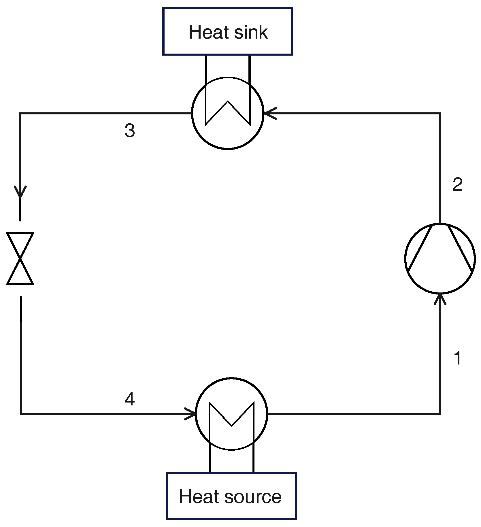
2.2. Reference Cycle

2.2.1. Thermodynamic States

Figure 1 shows a schematic layout of a CO2 transcritical heat pump in its fundamental configuration (the liquid receiver is not included for simplicity, as it does not affect the cycle under nominal operating conditions). The thermodynamic cycle can be calculated once four parameters are assigned:
  • Evaporation temperature T e v , with the corresponding pressure p e v = p s a t ( T e v ) ;
  • Superheating at the compressor inlet Δ T SH ;
  • Gas cooler pressure p g c ;
  • Temperature at the gas cooler exit T g c .
With the assumption of negligible pressure losses, the thermodynamic states are identified with the procedure described in the following paragraphs. First, the compressor inlet depends on the evaporation pressure and temperature and the required superheating:
p 1 = p e v
T 1 = T e v + Δ T SH .
The thermodynamic state at the compressor exit depends on the gas cooler pressure and the enthalpy reached by the refrigerant in the compression process:
p 2 = p g c
h 2 = h 1 + h ( p g c , s 1 ) h 1 / η s ,
where the isoentropic efficiency η s depends on the pressure ratio β = p g c / p e v according to Equations (4) and (5).
The temperature and pressure at the gas cooler exit are known:
p 3 = p g c
T 3 = T g c ,
and, finally, the thermodynamic state at the evaporator inlet is defined by the evaporation pressure and the isenthalpic process in the valve:
p 4 = p e v
h 4 = h 3 .

2.2.2. Cycle Performance

The heat and work transfer per unit mass of refrigerant fluid are given by:
Q g c = h 2 h 3 ,
Q e v = h 1 h 4 ,
W = h 2 h 1 ,
and the thermodynamic cycle and overall heat pump coefficient of performance (COP) are:
COP t h = Q g c / W ,
COP = η m COP t h .
The refrigerant fluid mass flow rate in the gas cooler is determined by the enthalpy change and the required rate of heat transfer:
m ˙ = Q ˙ g c / Q g c = Q ˙ g c / h 2 h 3 .
Exergy losses per unit mass in each component are calculated as follows:
E l , c = T 0 s 2 s 1
E l , g c = T 0 1 / T ¯ w 1 / T ¯ CO 2 , g c Q g c
E l , v = T 0 s 4 s 3
E l , e v = T 0 1 / T ¯ CO 2 , e v 1 / T ¯ a Q e v ,
where T 0 = 298.15   K is the thermodynamic reference temperature. The average temperature T ¯ in a constant-pressure heat transfer process is the ratio of enthalpy to entropy change:
T ¯ | a b = h b h a / s b s a
The exergy entering the cycle is:
E i n = E Q e v + W = 1 T 0 / T ¯ a Q e v + W
while the useful exergy produced by the heat pump is the exergy associated to the heat transfer in the gas cooler:
E o u t = E Q g c = 1 T 0 / T ¯ w Q g c .
The second-law efficiency is defined as:
η II = E o u t / E i n ,
while the fraction of exergy lost in each component is
y i = E l , i / E i n .
Combining Equations (17) and (25)–(27) the following relationship among the COP, exergy efficiency, and air and water average temperatures is obtained:
η II = 1 T 0 / T ¯ w T 0 / T ¯ a 1 / COP t h T 0 / T ¯ a 1 ,
which is a monotonic function of COP when the average temperatures of the external fluids are constant.

2.2.3. Design Parameters

Of the four input parameters, listed in Section 2.2.1, required to calculate the thermodynamic cycle, only superheating Δ T SH and gas cooler pressure p g c can be considered as design parameters that can be freely chosen; the evaporation temperature and gas cooler exit temperature, instead, depend on the properties of the HTF fluid and the minimum temperature difference at the evaporator and the gas cooler. The evaporator temperature can be calculated explicitly as follows:
Δ T SH > Δ T a T e v = T a , i Δ T e v Δ T SH ;
Δ T SH Δ T a T e v = T a , i Δ T a Δ T e v .
The location of the pinch point in the gas cooler cannot be located a priori because the specific heat of CO2 changes rapidly for the typical pressure and temperature ranges of the gas cooler [40]. Therefore, the gas cooler exit temperature must be found iteratively to ensure that the minimum temperature difference between CO2 and water in the gas cooler is equal to the desired value Δ T e v :
T g c : T w ( x ) T CO 2 , g c ( x ) Δ T g c x [ 0 , 1 ] ,
with x representing the normalized rate of heat transfer. The temperature of both fluids within the gas cooler is given by the energy conservation equation written for a control volume that spans from the gas cooler cold side (corresponding to the CO2 exit) to the section of the heat exchanger, where a fraction x of the overall heat rate is transferred:
h w ( x ) = h w , i + x Q ˙ g c / m ˙ w ;
h CO 2 , g c ( x ) = h 3 + x Q ˙ g c / m ˙ .
Therefore, with the assumption of negligible pressure losses in the heat exchangers, the thermodynamic cycle underlying the operation at the rated conditions of a transcritical CO2 ASHP is determined by the following boundary conditions and design parameters:
1. 
Q ˙ g c : rate of heat transferred in the gas cooler;
2. 
T w , i : water inlet temperature at the gas cooler;
3. 
Δ T w : water temperature glide in the gas cooler;
4. 
Δ T g c : minimum temperature difference between CO2 and water in the gas cooler;
5. 
T a , i : air inlet temperature in the evaporator;
6. 
Δ T a : air temperature decrease in the evaporator;
7. 
Δ T e v : minimum temperature difference between air and CO2 in the evaporator;
8. 
Δ T SH : superheating at the compressor inlet;
9. 
η c : compressor overall efficiency;
10.
η m : compressor mechanical efficiency;
11.
p g c : gas cooler pressure.
Table 1 lists the values of the design parameters assumed in this analysis. The first column reports the range of values of the parameters that define the end-user temperature profile and the ambient temperature and that are the basis for the parametric analysis of cycle performance discussed in Section 3.2; the second column reports the values of the design parameters held constant in all calculations; and the last column reports the parameters required by the cycle with an ejector as described in Section 2.5.

2.2.4. Constrained Optimization

Of the eleven input parameters described above, three are related to the heat load and its temperature profile ( Q ˙ g c , T w , i , Δ T w ), one is a boundary condition related to ambient conditions ( T a , i ), two are design parameters related to the heat exchanger design that should be optimized from a techno-economic perspective ( Δ T g c , Δ T e v ; the superheating at the compressor inlet is dictated by the need to ensure that no liquid droplets are drawn by the compressor), and finally the two efficiencies are defined by the technological quality of the compressor and motor. Therefore, the only parameter that can be optimized to ensure maximum COP is the gas cooler pressure p g c . However, optimization must consider the constraint due to the pinch point in the gas cooler, Equation (32), so the constrained optimization problem can be formulated in this way:
p g c , o p t , T g c , o p t : COP ( p g c , o p t , T g c , o p t ) = max COP ( p g c , T g c )
min T HTF , g c ( x ) T CO 2 , g c ( x ) = Δ T g c ,
that is, finding the values of gas cooler pressure and exit temperature that result in the maximum COP while ensuring the constraint that the minimum temperature difference in the gas cooler is equal to the prescribed value.

2.3. Cycle with Internal Heat Exchanger

An IHX can be used to increase the evaporation temperature (thereby increasing the COP): the refrigerating fluid leaves the evaporator as saturated vapor (a flooded evaporator in conjunction with a liquid/vapor separator can be used to ensure this condition) and the required superheating is obtained in the IHX, where the hot fluid is the refrigerant flowing out of the gas cooler as shown in Figure 2.
Thanks to the IHX, the evaporation temperature and pressure are:
T e v = T a , i Δ T a Δ T e v
p e v = p s a t ( T e v ) .
Thermodynamic states can be calculated with the procedure described for the reference case (Section 2.2.1). The additional component (IHX) allows the vapor quality to be set at the exit of the evaporator ( x 6 = 1 ). The heat supplied in the gas cooler and compressor work per unit mass of refrigerant are still defined by Equations (14) and (16), while the heat per unit mass at the evaporator is Q e v = h 6 h 5 .
The exergy losses in the compressor, gas cooler, valve, and evaporator can be calculated with Equations (20)–(23), while the exergy loss in the IHX is given by:
E l , IHX = T 0 s 1 s 6 s 3 s 4 .
Again, the only optimization parameter is the gas cooler pressure, which must be found through the constrained optimization procedure delineated in the previous section.

2.4. Parallel Compression

The cycle with parallel compression features three pressure levels (gas cooler pressure p g c , intermediate pressure p i , and evaporation pressure p e v ), with the intermediate pressure reached at the exit of a high-pressure valve (Figure 3), where the fluid reaches saturation conditions and flows to a liquid/vapor separator: the saturated vapor leaving the separator is drawn by an auxiliary compressor that works with a reduced pressure ratio, while the saturated liquid flows to the IHX, low-pressure valve, evaporator and IHX, to be drawn by the main compressor. The streams from the main and auxiliary compressors are finally mixed before entering the gas cooler. In this case, there are three different flow rates of refrigerant fluid: the flow rate m ˙ e v flowing in the evaporator, the flow rate m ˙ a u x drawn by the auxiliary compressor, and the flow rate in the gas cooler, being the sum of the first two: m ˙ = m ˙ e v + m ˙ a u x . Taking the flow rate in the gas cooler as reference, the other flow rates can be identified with the relative flow rate m as indicated in Figure 3:
m = m ˙ a u x / m ˙ .
Under the assumption of steady-state operation, the vapor mass flow rate produced by the expansion in the high-pressure valve must be equal to the flow rate of saturated vapor leaving the separator:
m = x 4 = x ( p i , h 4 = h 3 ) .
The cycle performance can be assessed through the following equations:
Q g c = h 2 h 3
Q e v = 1 m h 11 h 10
W = 1 m h 8 h 1 + m h 9 h 5 .
Finally, the exergy losses are:
E l , c = 1 m T 0 s 8 s 1
E l , c , a u x = m T 0 s 9 s 5
E l , m i x = T 0 s 2 m s 9 1 m s 8
E l , g c = T 0 1 / T ¯ w 1 / T ¯ CO 2 , g c Q g c
E l , v , H P = T 0 s 4 s 3
E l , IHX = 1 m T 0 s 1 s 11 s 6 s 7
E l , v , L P = T 0 s 10 s 7
E l , e v = T 0 1 / T ¯ CO 2 , e v 1 / T ¯ a Q e v .

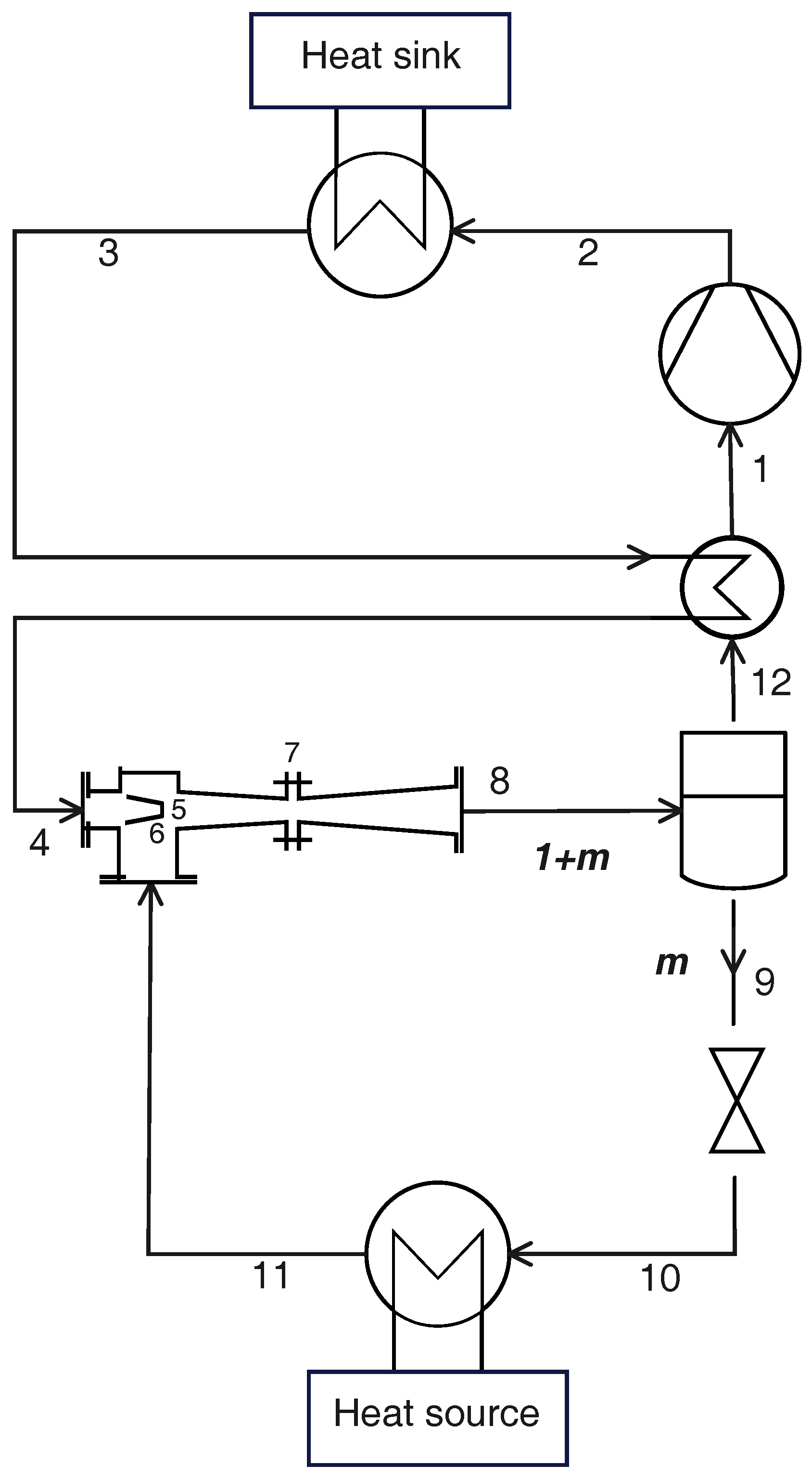
2.5. Cycle with Ejector

An ejector can be used in place of the high-pressure valve to avoid completely dissipating the fluid expansion. The fluid leaving the gas cooler (state 3 in Figure 4) first enters the IHX and then the ejector motive nozzle (state 4); the motive fluid expands to the suction pressure level p s (state 5), drawing fluid from the evaporator exit (state 11) through the suction nozzle. The two streams mix and enter the diffuser of the ejector (state 7), which increases the pressure to an intermediate pressure level p i . The resulting stream enters a liquid/vapor separator: the liquid (state 9) expands to a low-pressure valve and enters the evaporator (state 10), while the vapor (state 12) is superheated in the IHX and then is drawn by the compressor (state 1).
Three flow rates can be identified in this configuration: taking the mass flow rate in the gas cooler as reference, the ejector entrainment ratio is defined as the ratio of fluid drawn through the suction nozzle to the motive fluid:
m = m ˙ e v / m ˙ ;
as a result, the stream leaving the ejector has a relative mass flow rate m ˙ e j / m ˙ g c = 1 + m .
Under the assumption of steady-state operation, the mass flow rate of the saturated vapor leaving the separator ( m ˙ ) must be equal to the mass flow rate of vapor in the liquid/vapor mixture at the ejector exit [37]:
m ˙ = x 8 m ˙ e j m = 1 x 8 / x 8 .
The suction pressure can be selected through the design of the nozzles, and in this analysis, it is set at 95% of the evaporation pressure because it is demonstrated that the optimal suction pressure is close to the evaporation pressure [45]. The intermediate pressure level, instead, is not a design parameter but is established by the operation of the ejector as described in the following paragraphs.
Once the thermodynamic states at the evaporator exit (state 11) and the gas cooler exit (state 3) are identified, respectively, by the evaporation pressure and vapor quality ( p e v , x 11 = 1 ) and gas cooler pressure and exit temperature ( p g c , T g c ), the thermodynamic states involved in the operation of the ejector are found iteratively, taking the intermediate pressure p i and the entrainment ratio m as test variables.
The saturated vapor out of the separator (state 12) is identified by the intermediate pressure ( p 12 = p i ) and the vapor quality x 12 = 1 , and the fluid drawn by the compressor (state 1) is at the intermediate pressure ( p 1 = p i ) with the required level of superheating ( T 1 = T 12 + Δ T SH ); the heat per unit supplied to the cold fluid in the IHX is Q IHX = h 1 h 12 .
The fluid entering the motive nozzle (state 4) is at the gas cooler pressure ( p 4 = p g c ), and its enthalpy is deduced from the IHX energy conservation ( h 4 = h 3 Q IHX ). The irreversible adiabatic expansion in the motive nozzle leads to state 5, identified by the suction pressure ( p 5 = p s ) and the enthalpy h 5 = h 4 η m n h 4 h ( p 5 , s 4 ) , with η m n being the isentropic efficiency of the motive nozzle. Analogously, at the suction nozzle exit (state 6), the thermodynamic state is identified by the same suction pressure ( p 6 = p s ) and the enthalpy h 6 = h 11 η s n h 11 h ( p 6 , s 11 ) , with η s n being the isentropic efficiency of the suction nozzle.
With the assumption of negligible kinetic energy at the nozzle inlet [37], the velocity at the motive and suction nozzle exit is given by:
c 5 = 2 h 4 h 5
c 6 = 2 h 11 h 6 .
The velocity of the mixed stream entering the diffuser is given by the momentum conservation equation:
m ˙ 7 c 7 = m ˙ 5 c 5 + m ˙ 6 c 6 c 7 = c 5 + m c 6 / 1 + m .
Neglecting the kinetic energy at the ejector exit (state 8), this thermodynamic state is identified by the intermediate pressure level ( p 8 = p i ) and the enthalpy resulting from the energy conservation equation applied to the entire ejector ( h 8 = h 4 + m h 11 / 1 + m ); the resulting vapor quality can thus be calculated as x 8 = x ( p 8 , h 8 ) . The fluid entering the diffuser (state 7) is at the suction pressure ( p 7 = p s ) and the same total enthalpy of the diffuser exit ( h 7 = h 8 c 7 2 / 2 ). If the compression in the diffuser were isentropic, the enthalpy at the ejector exit would be h 8 ( s ) = h 7 + η d h 8 h 7 , where η d is the diffuser isentropic efficiency.
The procedure then checks the values of the intermediate pressure and entrainment ratio calculating the error against the first guess values, iterating until it is below the required threshold:
δ p i = p i p ( h 8 ( s ) , s 7 )
δ m = m 1 x 8 / x 8 ,
Finally, the remaining thermodynamic states can be calculated as follows. At the compressor exit (state 2), the fluid is at the gas cooler pressure ( p 2 = p g c ), and its enthalpy is h 2 = h 1 + h ( p 2 , s 1 ) h 1 / η s . The saturated liquid leaving the separator (state 9) is identified by the intermediate pressure ( p 9 = p i ) and the vapor quality ( x 9 = 0 ), while the liquid at the low-pressure valve exit (state 10) is at the evaporator pressure ( p 10 = p e v ) and the same enthalpy as it had at the valve inlet ( h 10 = h 9 ).
The heat and work per unit mass are given by the following equations:
Q g c = h 2 h 3
Q e v = m h 11 h 10
W = h 2 h 1 ,
while the exergy losses are:
E l , c = T 0 s 2 s 1
E l , g c = T 0 1 / T ¯ w 1 / T ¯ CO 2 , g c Q g c
E l , IHX = T 0 s 1 s 12 s 3 s 4
E l , e j = T 0 1 + m s 8 s 4 m s 11
E l , v = T 0 s 10 s 9
E l , e v = T 0 1 / T ¯ CO 2 , e v 1 / T ¯ a Q e v .

3. Results and Discussion

The thermodynamic cycles are first analyzed in detail in Section 3.1 with reference to two particular end-user temperature profiles, defined in Table 2 and labeled “Case A” and “Case B”, and with an ambient temperature T a , i = 0   ° C , to discuss the influence of the gas cooler pressure on the performance and, more specifically, to highlight the reasons for the existence of an optimal gas cooler pressure; the analysis is based on the reference cycle, but it also applies to the modified cycles, which show the same qualitative behavior. The discussion presented in the following paragraphs shows that Cases A and B represent end-user heat demands that result, respectively, in two pinch points or just one pinch point in the gas cooler for the optimized thermodynamic cycle. The performance of the optimal cycles is then discussed in Section 3.2 as the boundary conditions change in the full ranges defined in Section 2.1, considering all the cycle modifications described in the previous section.

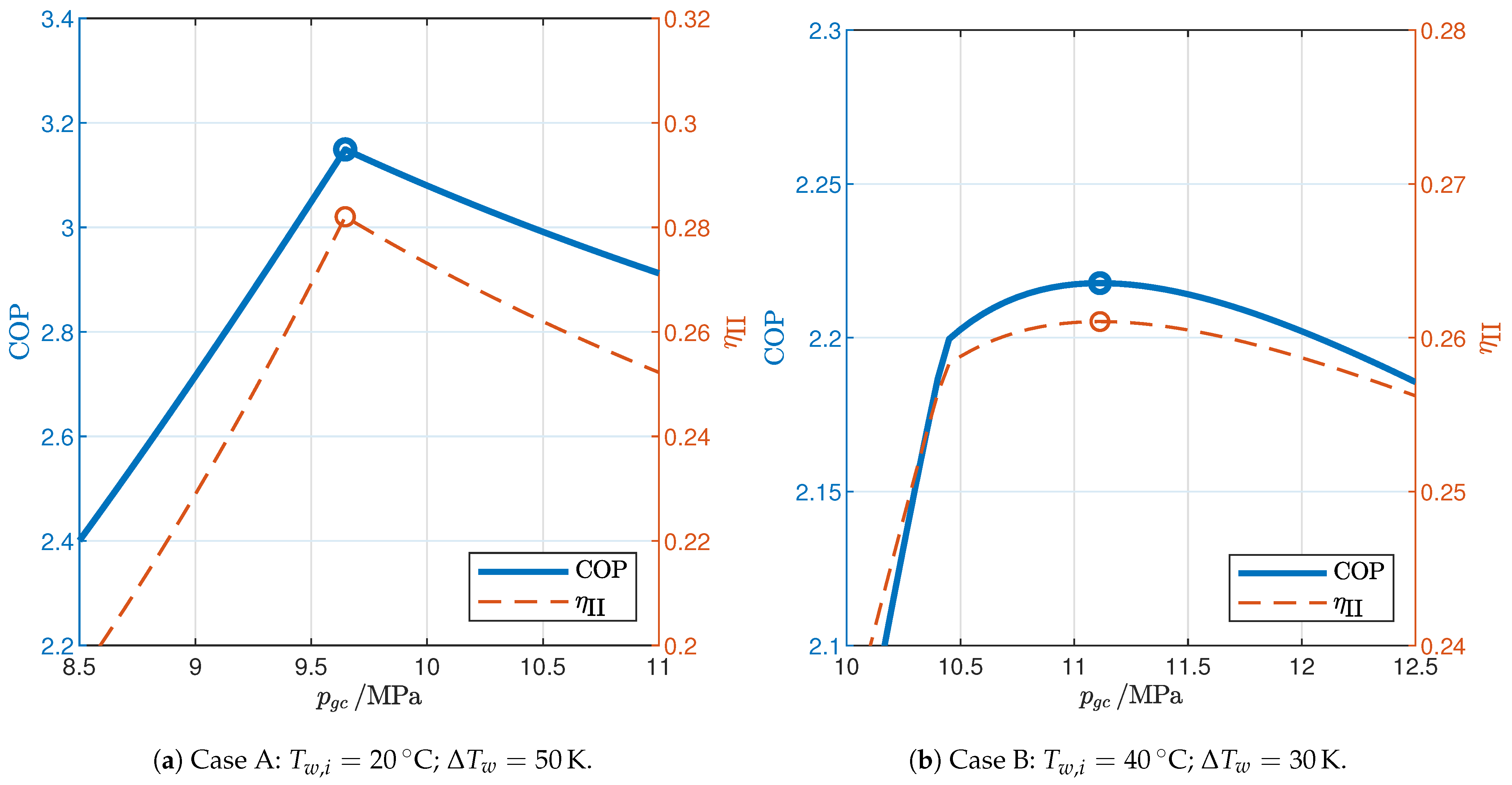
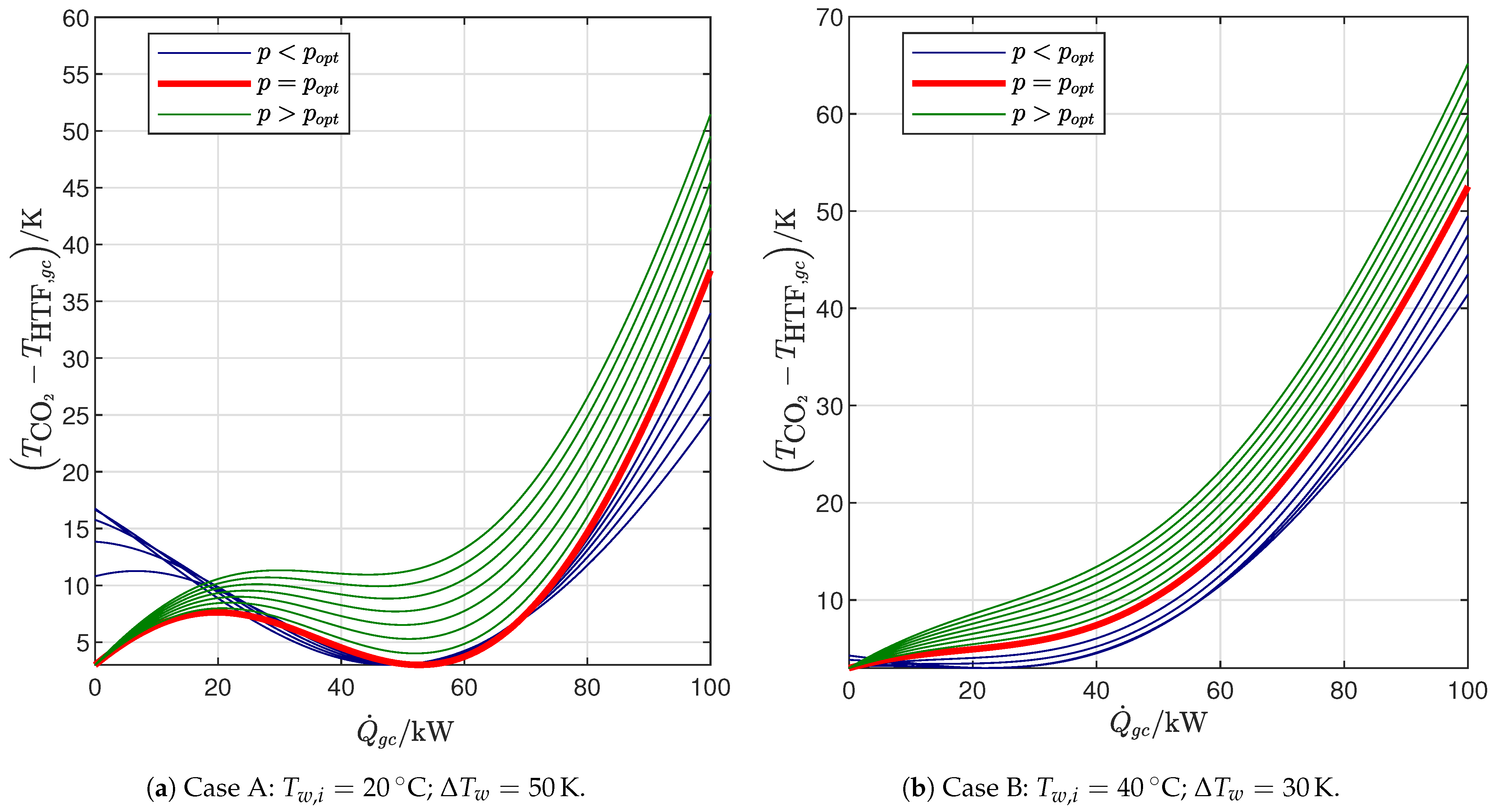
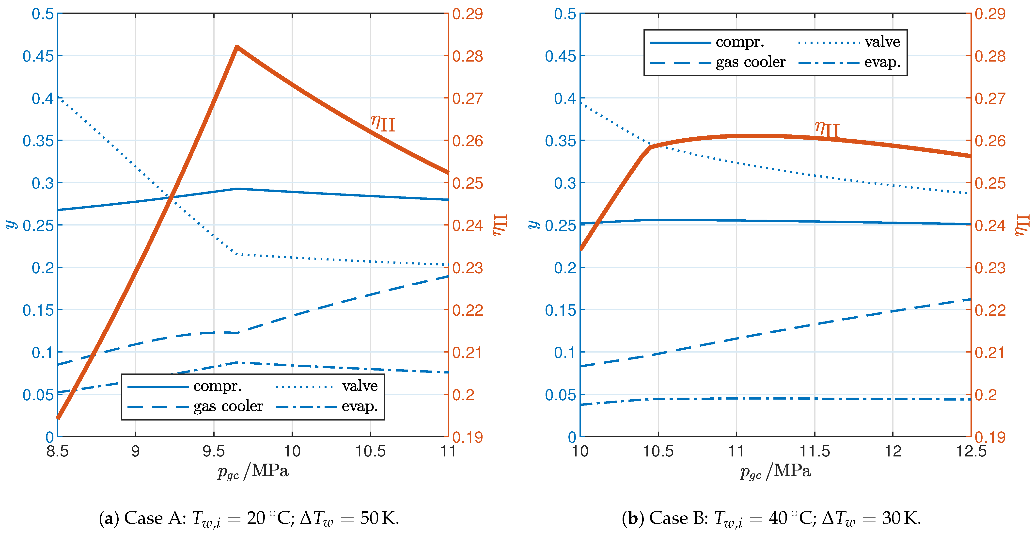
3.1. Influence of Gas Cooler Pressure (Cycle Optimization)

Figure 5 shows how the cycle COP and exergy efficiency change with the gas cooler pressure when the gas cooler exit temperature T g c is subject to the constraint represented by Equation (32), which ensures that the minimum temperature difference in the gas cooler is equal to the desired value ( Δ T g c ) . In both cases, the analysis reveals that there is a discontinuity in the slope of the curves that is explained by the temperature difference along the gas cooler represented in Figure 6: for low values of p g c , the pinch point is located inside the gas cooler, and the exit temperature progressively decreases with p g c , leading to an increase in COP, until a threshold pressure level is reached that gives rise to two pinch points, one inside the heat exchanger and the other at its cold end. In other words, the threshold pressure level that marks the discontinuity in the slope visible in Figure 5 is the lowest value of the gas cooler pressure that results in the lowest possible gas cooler exit temperature: T g c , min = T w i + Δ T g c . For higher values of p g c , the pinch point remains on the cold side, while the temperature differences inside the heat exchanger progressively increase.
However, the two cases differ with regard to the location of the maximum efficiency: in case A, representing end-user temperature profiles with relatively low inlet temperatures and high temperature glides, the optimal gas cooler pressure is exactly the threshold pressure level identified previously so that the maximum efficiency is reached for the configuration with the double pinch point (2PP) in the gas cooler (Figure 6a; this is the situation most commonly described in the literature by pinch-point analyses of transcritical CO2 cycles [23,46]); in case B, representing end-user temperature profiles with relatively high inlet temperatures and low temperature glides, there is only one pinch point (1PP) located at the cold end of the heat exchanger (Figure 6b) as also observed by Cui et al. [41], and the optimal pressure is higher than the threshold pressure that results in T g c = T g c , min .
The analysis of the irreversibility generated in each component (Figure 7) explains the different behavior in the two cases. The change in efficiency due to the gas cooler pressure is mainly a result of the exergy losses in the valve and the gas cooler since the losses in the evaporator and the compressor are much less variable with p g c . In both cases, the optimal gas cooler pressure represents the best trade-off between the losses in the valve, which decrease with an increase in p g c , and those in the gas cooler, which generally do the opposite. As for the valve, an increase in p g c at first rapidly lowers the exit temperature from the gas cooler (Figure 6) leading to a significant reduction in the entropy at the valve inlet (state 3; see Figure 8), which explains why the exergy loss in the valve also rapidly decreases (Equation (22)); when the pinch point reaches the cold end of the gas cooler, the exit temperature no longer changes, and the entropy at the valve inlet still decreases with p g c but with a much reduced slope. This general trend is observed in both cases; however, it is more pronounced in case A (Figure 7a) than in case B (Figure 7b) due to the different slope of the constant-temperature lines corresponding to the different values of T g c , min in the two cases (Figure 8): in case A, the entropy at the valve inlet is almost constant when the gas cooler exit temperature does not change, while in case B, the change in entropy is not negligible even with a constant T g c . As a result, the exergy loss in the valve in case B still decreases significantly even after the threshold pressure for the 2PP region has been reached. On the other hand, Figure 6 shows that the average temperature of CO2 in the gas cooler generally increases with the gas cooler pressure, leading to greater exergy losses in the gas cooler as dictated by Equation (21). Therefore, exergy losses in the valve and the gas cooler are significantly influenced by the gas cooler pressure with opposite trends: this is ultimately the reason why an optimal gas cooler pressure exists. Moreover, in case B, the optimal pressure is higher than the threshold pressure because the valve exergy loss still decreases markedly after the threshold pressure has been reached, while in case A, the optimal and threshold pressure levels are the same.
This analysis shows that it is necessary to consider the exergy balance of the entire cycle, with particular regard to the exergy destruction in the valve and the gas cooler, to fully explain the behavior of the optimal gas cooler pressure; previous studies identified the optimal pressure focusing on the irreversibility of the gas cooler without acknowledging the relevance of the irreversibility in the valve [40,41].

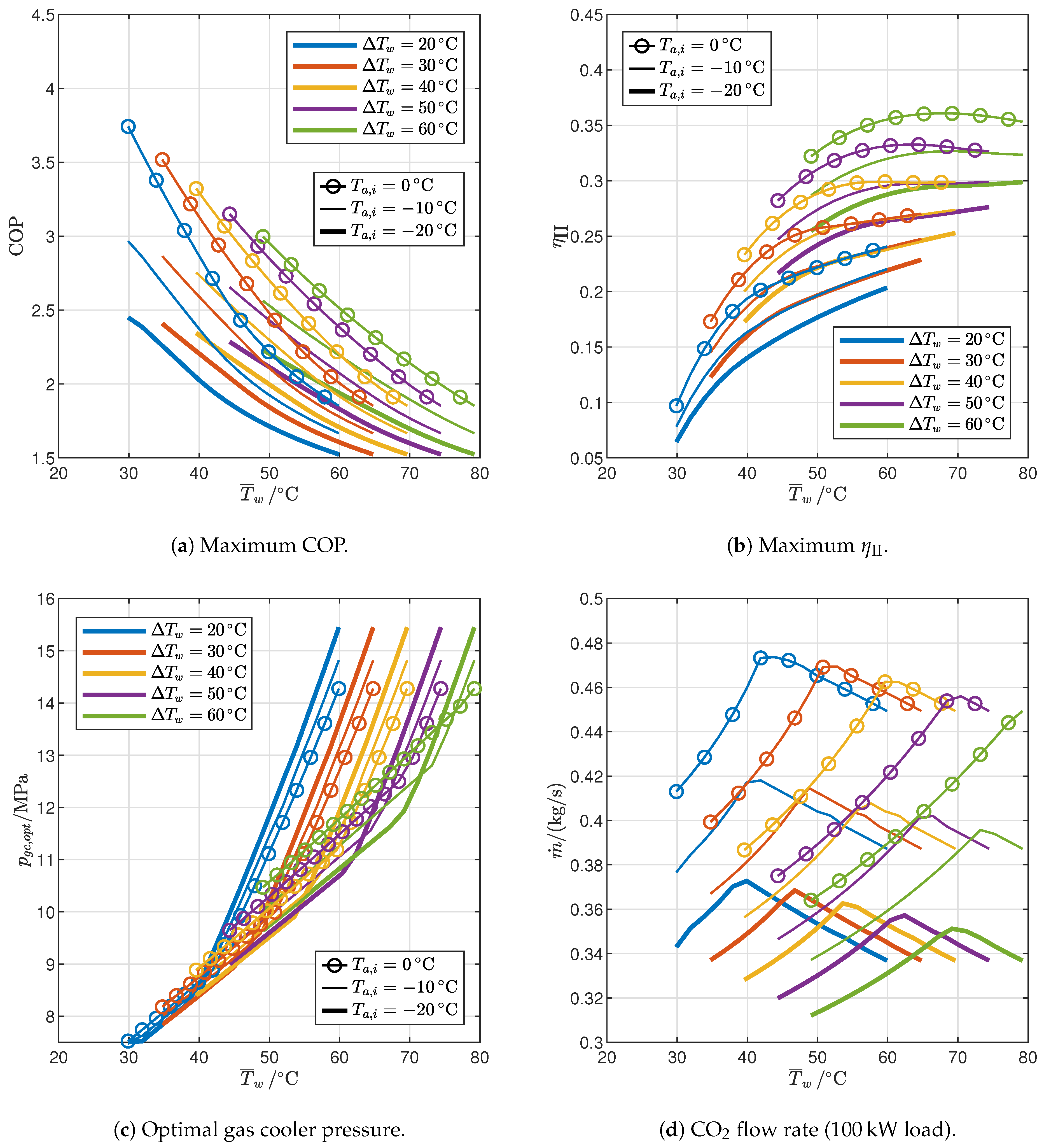
3.2. Optimized Cycles: Influence of End-User Temperature Profile and Ambient Temperature

3.2.1. Reference Cycle

The performance of the optimized reference cycle is illustrated in Figure 9 with reference to the maximum values of COP and second-law efficiency that can be achieved by choosing the optimal gas cooler pressure for different end-user temperature profiles (represented by water average temperature and temperature glide) and ambient temperatures (air inlet temperature at the evaporator). The average water temperature is calculated as the thermodynamic average ( T ¯ w = Δ h w / Δ s w ); however, it is very close to the arithmetic average between gas cooler inlet and exit due to the properties of water in the region of interest.
The maximum coefficient of performance (Figure 9a) follows trends that can be easily explained with reference to the general behavior of inverse cycles: it increases with an increase in ambient temperature (which drives the evaporation temperature upward) or with a decrease in the average water temperature; moreover, it increases with the temperature glide since the CO2 temperature profile during the heat rejection process is more suitable for relatively steep end-user temperature profiles as it is well documented in the literature [47]. However, the second-law efficiency (Figure 9b) shows opposite trends, revealing that when the COP decreases, it is because it is driven by a change in the boundary conditions, even though the irreversibility generated is lower. The range of COP that can be achieved by the reference cycle is 1.52–3.74 for the boundary conditions indicated in Table 1; the second-law efficiency range is 6.4–36.1%.
The effect of boundary conditions on the optimal value of gas cooler pressure is shown in Figure 9c. For a given temperature glide, it increases with the average water temperature, and the trend is clearly split into two regions: both display a linear dependence between p g c , o p t and T ¯ w but with a significantly different slope. The analysis carried out in the previous section explains the different behavior: for end-user temperature profiles with a relatively low water inlet temperature and high temperature glide, represented by case A (Table 2), the optimal gas cooler pressure is the one that gives rise to a double pinch point (2PP) in the gas cooler (Figure 6a), which increases relatively slowly with the average water temperature (less steep regions in Figure 9c); when the water inlet temperature is relatively high and the temperature glide relatively low (such as in case B, Table 2), instead, the optimal gas cooler pressure generates a single pinch point in the gas cooler (Figure 6b) and increases much faster with the average water temperature. Figure 9c also shows that the temperature glide does not significantly affect the optimal gas cooler pressure in the low-slope region (which will be indicated as the 2PP region from now on) while it is much more relevant in high-slope regions (1PP region), where the optimal gas cooler pressure increases with a decrease in the temperature glide for the same average water temperature. In general, the optimal gas cooler pressure can be as high as approximately 15.4 M Pa in the case of high-temperature heat demands.
Figure 9d shows the trend of the working fluid flow rate required by the reference cycle to supply a constant 100 kW load; thus, according to Equation (19), the flow rate is inversely proportional to the heat transferred to the gas cooler per unit mass ( Q g c = h 2 h 3 ). The flow rate trend is clearly split into two regions as in the case of the gas cooler pressure: in the 2PP region, the flow rate increases with the average water temperature, while it decreases with T ¯ w in the 1PP region. This behavior is explained by Figure 10, which shows the optimized reference cycles for different water inlet temperatures, holding the water temperature glide and the air inlet temperature constant. In the 2PP region, the gas cooler exit moves quickly to the right as T ¯ w increases, faster than the gas cooler inlet: as a result, the heat per unit mass Q g c decreases and the flow rate increases. In contrast, in the 1PP region, the gas cooler pressure rises much faster (Figure 9c), so the enthalpy at the gas cooler inlet increases faster than at the exit, leading to an increase in Q g c and a consequent decrease in flow rate.
The impact of the irreversibility of each component on the performance of the reference cycle is described in Figure 11, which shows the exergy losses y taking place in each component. The compressor (Figure 11a) introduces substantial exergy losses (23.5–33.6%) due to its relatively low efficiency; however, the losses decrease monotonically with the average water temperature, and also decrease with the water temperature glide, and an increase in ambient temperature is slightly beneficial. The losses in the gas cooler (Figure 11b) and in the valve (Figure 11c) show instead two different behaviors for the 2PP and 1PP regions since they depend on the gas cooler exit state (Figure 10). In particular, in the 2PP region, the exergy loss in the gas cooler decreases with the average water temperature thanks to a reduced variability in the specific heat of CO2, which makes the temperature difference inside the gas cooler less variable between the two pinch points (see Figure 6a). On the other hand, in the 1PP region, as the optimal gas cooler pressure increases, the temperature profiles of CO2 and water diverge, resulting in increasing irreversibility. Opposite trends can be observed for the exergy loss in the valve (Figure 11c), which increases with the average water temperature in the 2PP region, while it is almost flat in the 1PP region. Finally, exergy losses in the evaporator are the smallest (2.5–12.1%), given the relatively close temperature profiles, and decrease monotonically with the average water temperature; evaporator exergy losses decrease when the ambient temperature or the water temperature glide decrease.

3.2.2. Cycle Modifications

The simplest modification to the reference cycle is the introduction of the IHX discussed in Section 2.3, which improves the performance by raising the evaporation temperature by Δ T SH Δ T e v equal to 2 K with the assumptions made in this study, as indicated by Equations (30) and (37), since the required superheating is supplied by the IHX instead of the evaporator. The corresponding reduction in entropy generation in the evaporator explains the increase in COP by 1.7–5.2% shown in Figure 12a, and in second-law efficiency (Figure 12b) by 2.3–8.5%. The increase in efficiency falls with an increase in the average water temperature, with different slopes in the 2PP and 1PP regions (steeper in 1PP), indicating that the IHX is particularly beneficial in those conditions where the second-law efficiency of the reference cycle is lower (Figure 9b); moreover, the IHX is more effective for high temperature glides and ambient temperatures. It is worth observing that in the literature, it has been reported that the IHX can in some circumstances increase COP while at the same time reducing exergy efficiency [28]: however, this can only be possible under different assumptions (with particular regard to the temperature profile of external fluids) because COP and exergy efficiency are related by Equation (29), which is a monotonic function if the average temperatures of external fluids are constant.
The optimal gas cooler pressure (Figure 12c) is almost the same as in the reference cycle: it is higher in the 2PP region ad lower in the 1PP region by approximately around 0.5–1%. The mass flow rate (Figure 12d) is instead always slightly higher than in the reference cycle due to the reduced enthalpy at the gas cooler inlet (see Figure A1 and Figure A2), but the increase is just 1.5–2% in the 2PP region and 2.5–3% in the 1PP region.
The results obtained with the cycles with IHX and PC (Section 2.4) or with IHX and ejector (Section 2.5) are illustrated in Figure 13, Figure 14 and Figure 15. Figure 13 shows how the end-user temperature profile and the ambient temperature affect the COP (Figure 13a,b) and the second-law efficiency (Figure 13c,d) of the two cycles. It must be observed that, since the two cycles include an IHX, some of the performance increase must be attributed to that component as discussed with reference to Figure 12. The additional improvement is generally produced by the reduction in exergy losses in the expansion through the valve: in the case of PC, thanks to a fraction of the flow rate undergoing only part of the expansion; in the case of the ejector, thanks to the energy recovery in the high-pressure expansion through the motive nozzle.
The cycle with the IHX and ejector produces the highest performance improvement: the COP increases by 13.3–26.1% (Figure 13b), and the second-law efficiency increases by 21.0–37.6% (Figure 13d), compared to 6.1–20.0% and 8.3–33.2% for the COP and second-law efficiency of the cycle with IHX and PC (Figure 13a,c). Again, the trend with respect to the average water temperature is different for the 2PP and 1PP regions: the efficiency increases with T ¯ w in the former and decreases in the latter. The cycle with ejector is less sensitive to ambient temperature than the cycle with PC since the COP is almost constant with T a , i in the 2PP region; however, the ambient temperature has opposite effects on the improvement in efficiency of the two cycles, which decreases with T a , i in the cycle with PC while it increases in the cycle with the ejector. Finally, in both cases, the improvement is greatest for low values of temperature glide: indeed, the performance of the reference cycle is already relatively good with large temperature glides, so the cycle modifications are more effective where the reference cycle is weakest.
Figure 14 illustrates the optimal gas cooler pressure and the intermediate pressure for the two cycles. It is worth recalling that the intermediate pressure is a design parameter that can be optimized only in the case of the cycle with PC; in the cycle with an ejector, it is instead a result of the mass balance at the liquid/vapor separator at steady state. For both cycles, the optimal gas cooler pressure (Figure 14a,b) is again very similar to that of the reference cycle: in particular, it is higher in the 2PP region and lower in the 1PP region but, in any case, by less than 1%. The intermediate pressure level is higher in the cycle with PC (Figure 14c) than in the cycle with the ejector (Figure 14d), and it generally increases with the average water temperature, although with a low slope in the 1PP region of the cycle with PC. Moreover, for both cycles, the intermediate pressure falls with a decrease in ambient temperature or an increase in the temperature glide.
Finally, Figure 15 shows the mass flow rates in the optimized cycles with the IHX and PC or ejector. In both cases, the mass flow rate in the gas cooler (Figure 15a,b) must increase with respect to the reference cycle due to the reduced enthalpy at the gas cooler inlet (Figure A1 and Figure A2), and the increase is much higher in the 1PP region (up to 35–45%) than in the 2PP region (where it is around 5–15%). Figure 15c shows the fraction of the flow rate compressed by the auxiliary compressor in the cycle with PC, which is quite sensitive to the design parameters: it is in the range 15–52%, increasing with an increase in the average water temperature, a decrease in the temperature glide, or a decrease in the ambient temperature. The entrainment ratio in the cycle with ejector is also very sensitive to the design parameters, varying in the range 45–81%. However, the effect of the design parameters is the opposite: the entrainment ratio increases with a decrease in the average water temperature, an increase in the temperature glide, or an increase in the ambient temperature.

4. Conclusions

This article presents the energy and exergy analysis of transcritical CO2 cycles for ASHP applications, considering water as the heat sink in the gas cooler, with regard to different rated operating conditions (inlet temperature and temperature glide of water in the gas cooler, air inlet temperature in the evaporator) and different layouts in addition to the reference cycle: with IHX; with IHX and ejector; and with IHX and parallel compression. The following remarks summarize the most relevant conclusions that can be drawn from the results presented and discussed in the previous section.
1.
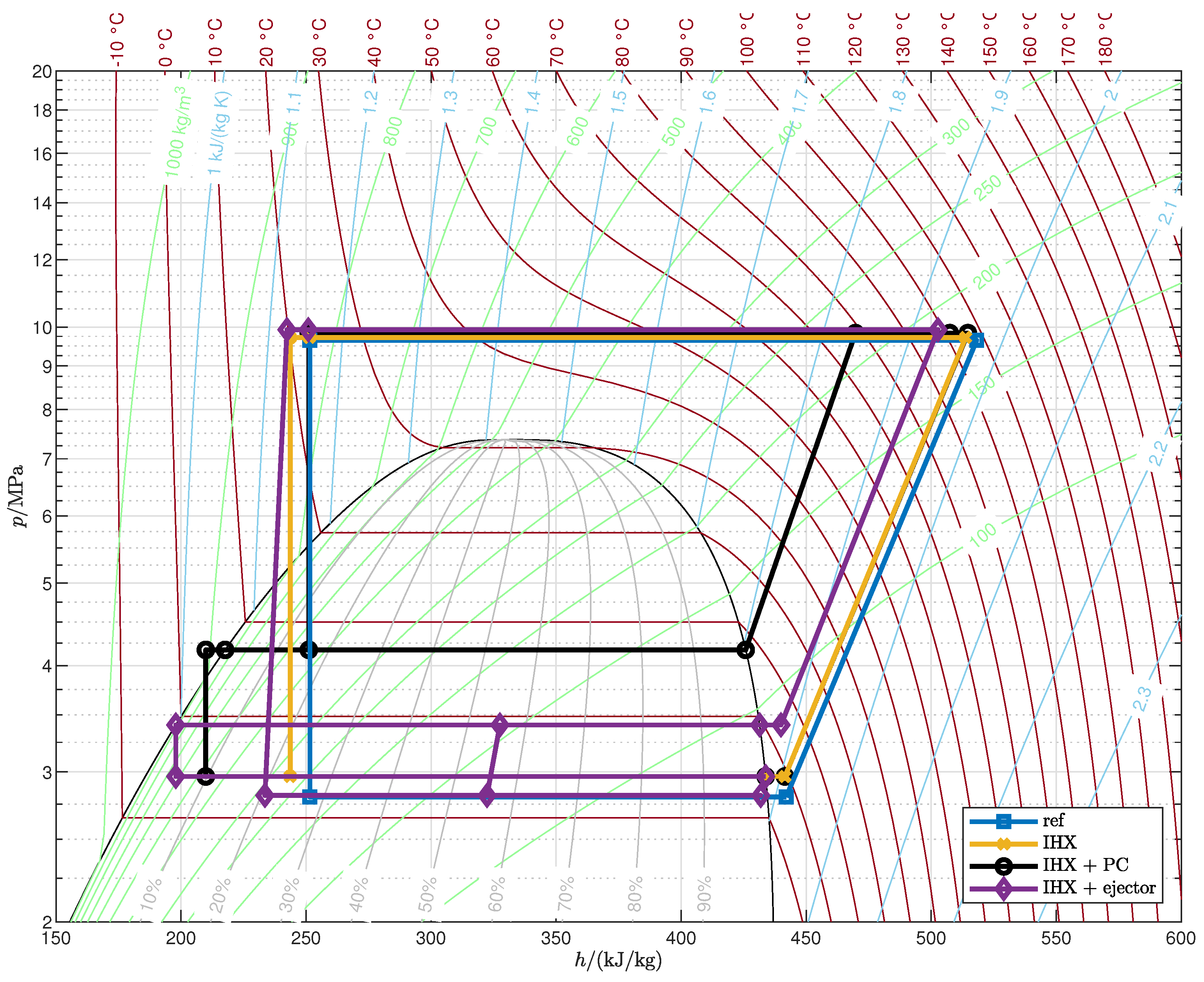
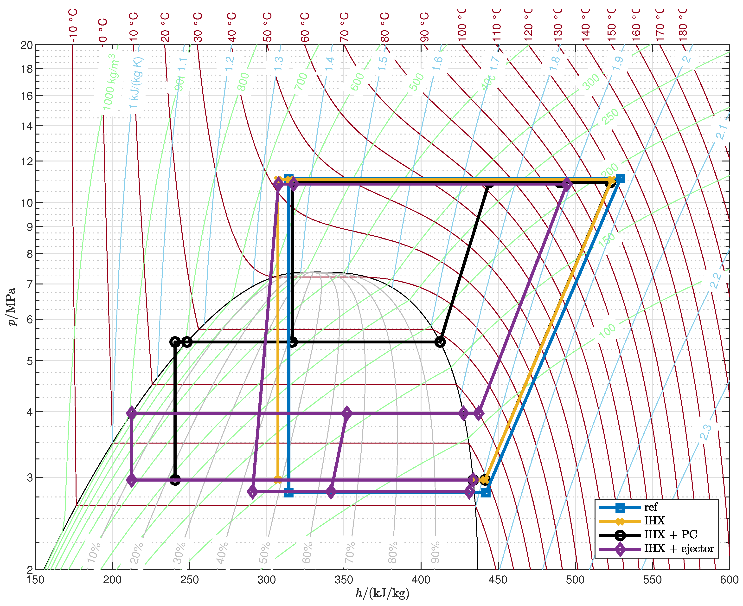
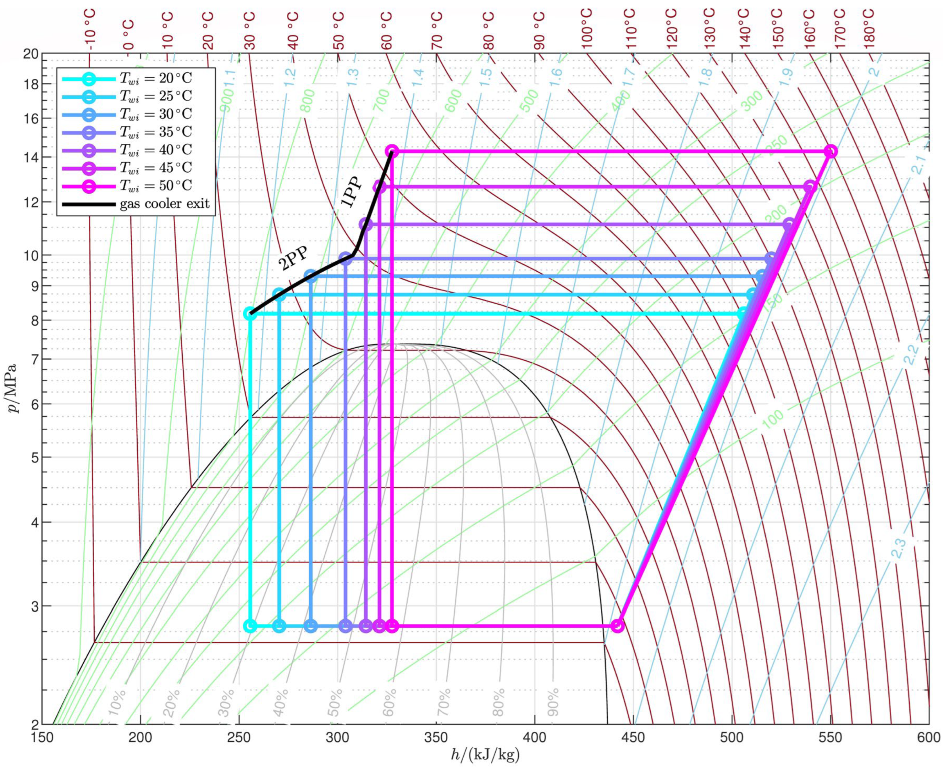
The temperature profile of the end user determines the number and locations of pinch points in the gas cooler for the maximum COP configuration: for relatively low inlet temperature and high temperature glides, the optimal pressure is the one that gives rise to two pinch points, one at the cold end and another inside the gas cooler (2PP configurations), while for relatively high inlet temperatures and low temperature glides, the optimal pressure is higher than the one that results in two pinch points, and in the optimal configuration, there is only one pinch point in the gas cooler, located at the cold end (1PP configurations).
2.
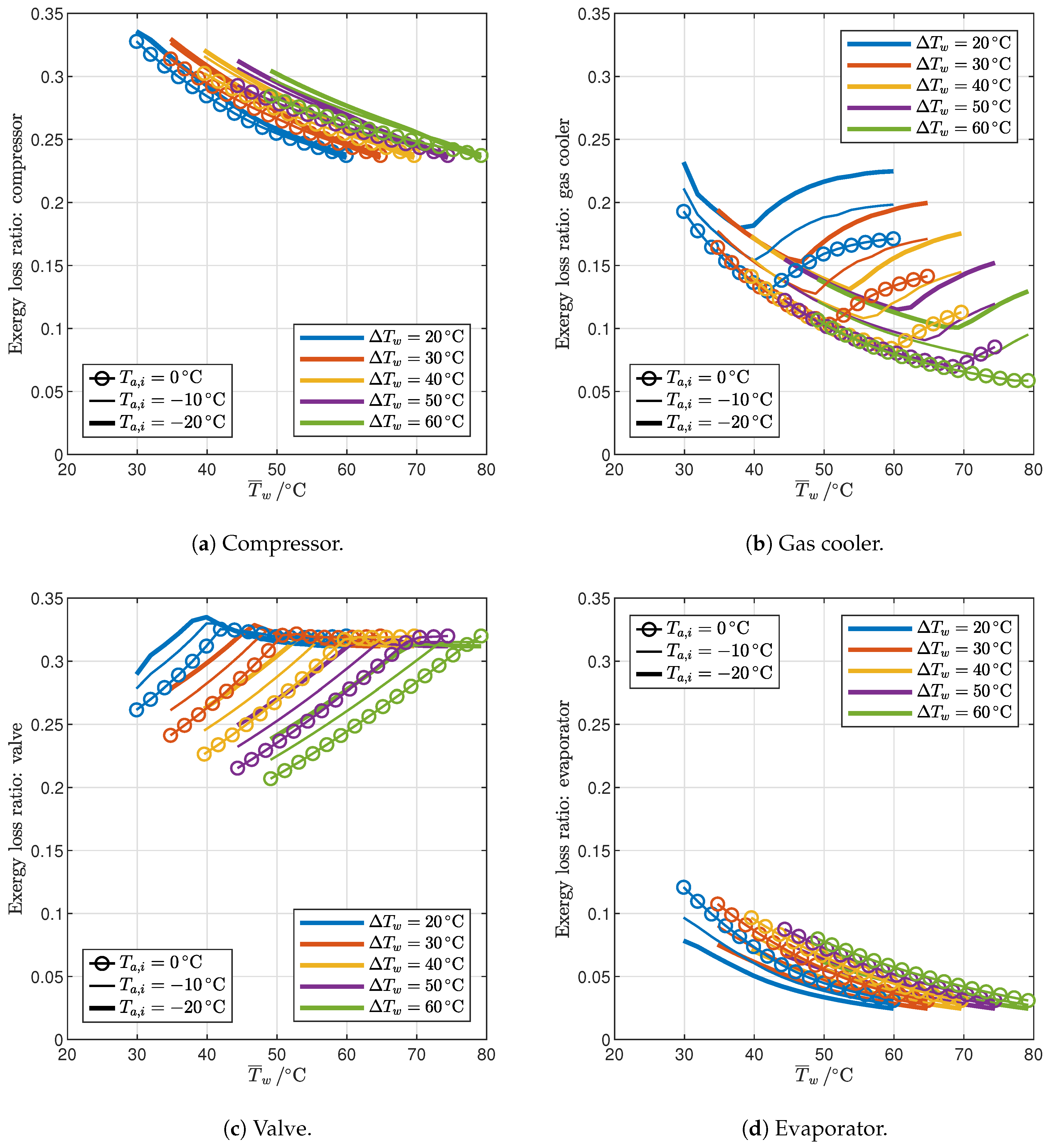
The transition from the 2PP to the 1PP region mainly depends on the average water temperature and the temperature glide, and is explained by the exergy destruction that takes place not only in the gas cooler but also in the valve.
3.
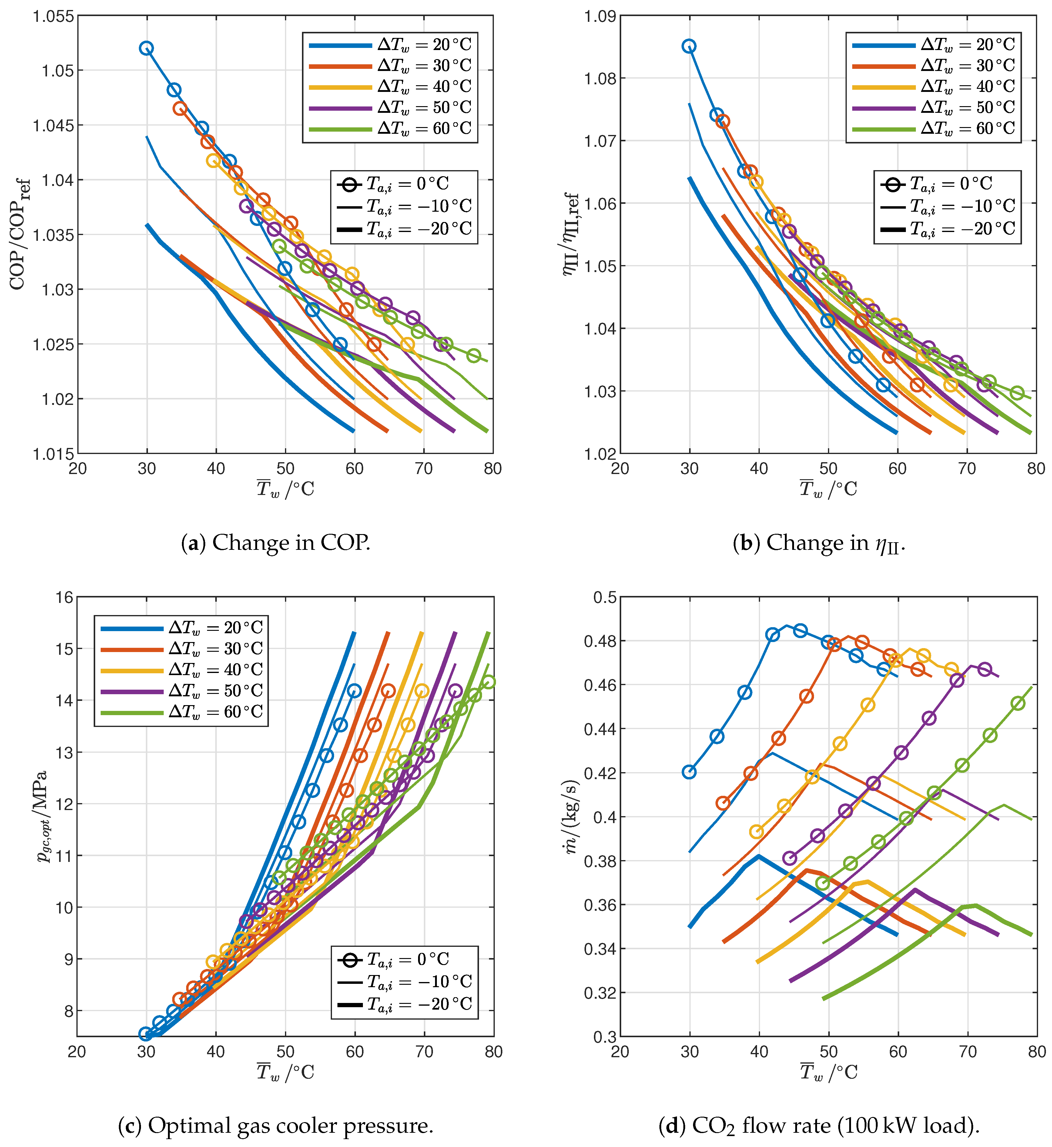
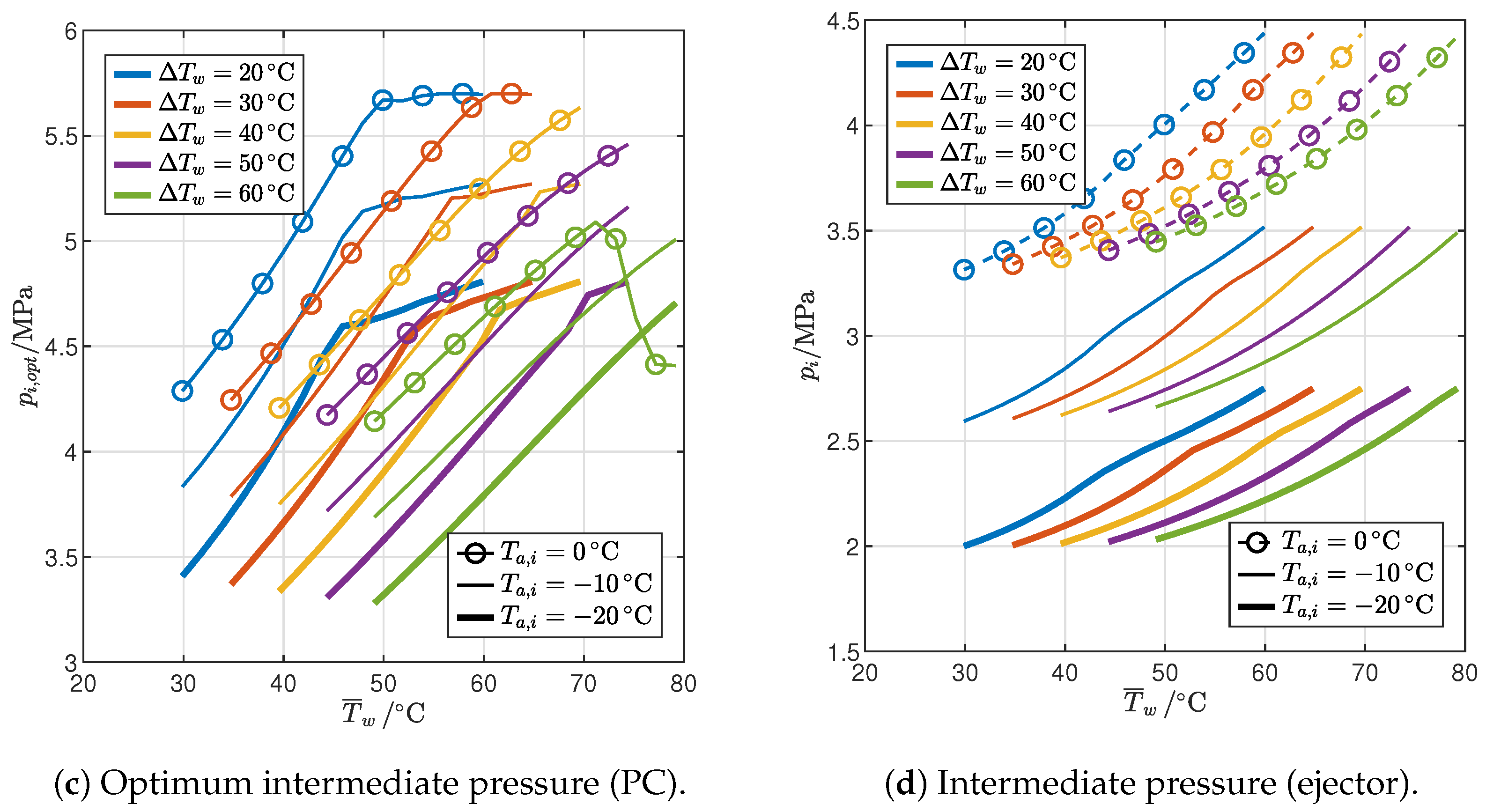
The optimal gas cooler pressure increases with the average water temperature but at different rates in the 2PP and 1PP regions. In particular, the rate of increase is much higher for 1PP configurations.
4.
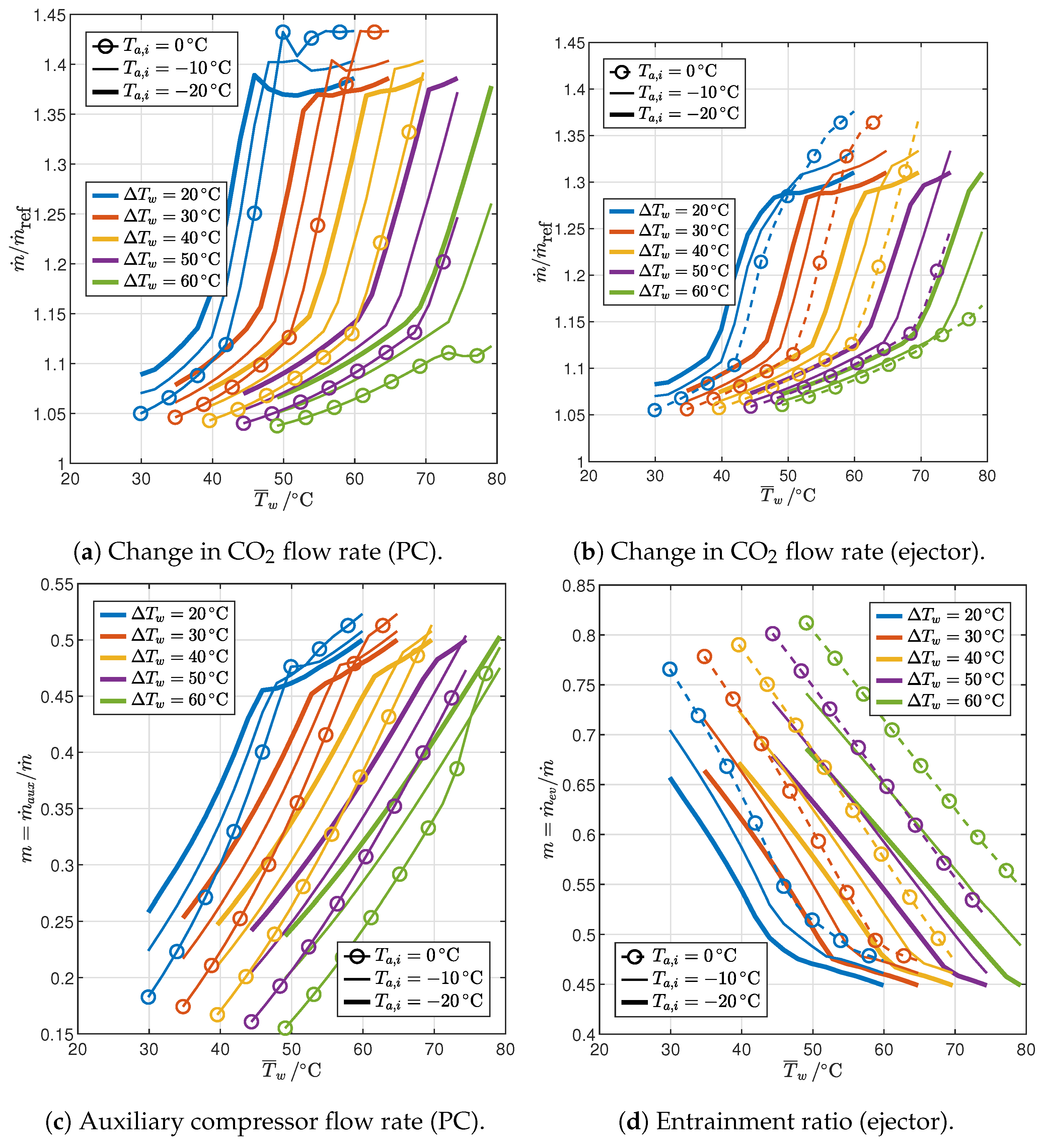
The flow rate of CO2 changes with the average water temperature in different ways in the 2PP and 1PP regions: it increases in the former and decreases in the latter. Furthermore, it decreases with the ambient air temperature.
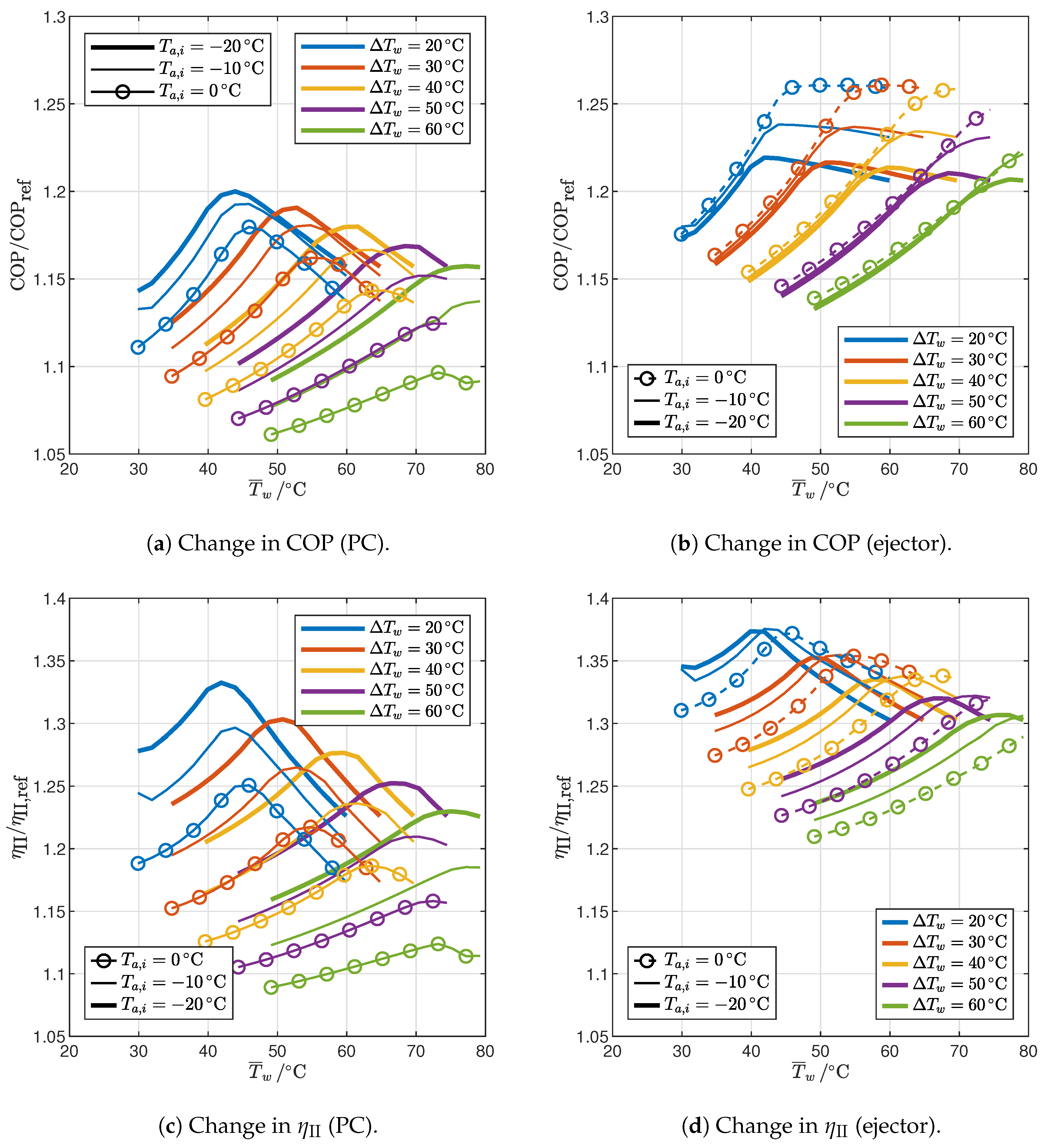
5.
The cycle with IHX and ejector is the most efficient among those analyzed: with respect to the reference cycle, the COP increases by 13.3–26.1% and the second-law efficiency by 21.0–37.6%, depending on the operating conditions.

Author Contributions

Conceptualization, M.M.; methodology, M.M.; software, M.M.; validation, M.G., M.M. and M.V.; formal analysis, M.M.; investigation, M.M.; writing—original draft preparation, M.M.; writing—review and editing, M.G., M.M. and M.V.; visualization, M.G., M.M. and M.V.; project administration, M.M.; funding acquisition, M.M. All authors have read and agreed to the published version of the manuscript.

Funding

This research was funded by the Ministry of Enterprises and Made in Italy, project n. F/350182/01-02/X60.

Data Availability Statement

The original contributions presented in the study are included in the article.

Conflicts of Interest

The authors declare no conflicts of interest.

Abbreviations

The following abbreviations are used in this manuscript:
1PPConfigurations with optimal pressure resulting in one gas cooler pinch point
2PPConfigurations with optimal pressure resulting in two gas cooler pinch point
ASHPAir Source Heat Pump
COPCoefficient Of Performance
HTFHeat Transfer Fluid
HPHeat Pump
IHXInternal Heat Exchanger
PCParallel Compression

Appendix A. Optimized Thermodynamic Cycles

Figure A1. Optimized cycles (case A).
Sustainability 16 07511 g0a1
Figure A2. Optimized cycles (case B).
Sustainability 16 07511 g0a2

References

  1. International Energy Agency. The Future of Heat Pumps; OECD: Paris, France, 2022. [Google Scholar] [CrossRef]
  2. Bellocchi, S.; Manno, M.; Noussan, M.; Prina, M.G.; Vellini, M. Electrification of Transport and Residential Heating Sectors in Support of Renewable Penetration: Scenarios for the Italian Energy System. Energy 2020, 196, 117062. [Google Scholar] [CrossRef]
  3. Simon, S.; Xiao, M.; Harpprecht, C.; Sasanpour, S.; Gardian, H.; Pregger, T. A Pathway for the German Energy Sector Compatible with a 1.5 °C Carbon Budget. Sustainability 2022, 14, 1025. [Google Scholar] [CrossRef]
  4. Gaur, A.S.; Fitiwi, D.Z.; Curtis, J. Heat Pumps and Our Low-Carbon Future: A Comprehensive Review. Energy Res. Soc. Sci. 2021, 71, 101764. [Google Scholar] [CrossRef]
  5. Faraldo, F.; Byrne, P. A Review of Energy-Efficient Technologies and Decarbonating Solutions for Process Heat in the Food Industry. Energies 2024, 17, 3051. [Google Scholar] [CrossRef]
  6. Ong, B.H.Y.; Bhadbhade, N.; Olsen, D.G.; Wellig, B. Characterizing Sector-Wide Thermal Energy Profiles for Industrial Sectors. Energy 2023, 282, 129028. [Google Scholar] [CrossRef]
  7. Zuberi, M.J.S.; Hasanbeigi, A.; Morrow, W. Techno-Economic Evaluation of Industrial Heat Pump Applications in US Pulp and Paper, Textile, and Automotive Industries. Energy Effic. 2023, 16, 19. [Google Scholar] [CrossRef]
  8. Schoeneberger, C.; Dunn, J.B.; Masanet, E. Technical, Environmental, and Economic Analysis Comparing Low-Carbon Industrial Process Heat Options in U.S. Poly(vinyl chloride) and Ethylene Manufacturing Facilities. Environ. Sci. Technol. 2024, 58, 4957–4967. [Google Scholar] [CrossRef]
  9. United Nations. Montreal Protocol on Substances That Deplete the Ozone Layer. 1987. Available online: https://treaties.un.org/doc/Treaties/1989/01/19890101%2003-25%20AM/Ch_XXVII_02_ap.pdf (accessed on 15 July 2024).
  10. United Nations. Amendment to the Montreal Protocol on Substances That Deplete the Ozone Layer. 2016. Available online: https://treaties.un.org/doc/Treaties/2016/10/20161015%2003-23%20PM/Ch_XXVII-2.f-English%20and%20French.pdf (accessed on 15 July 2024).
  11. Wu, D.; Hu, B.; Wang, R.Z. Vapor Compression Heat Pumps with Pure Low-GWP Refrigerants. Renew. Sustain. Energy Rev. 2021, 138, 110571. [Google Scholar] [CrossRef]
  12. Zühlsdorf, B.; Jensen, J.K.; Elmegaard, B. Heat Pump Working Fluid Selection—Economic and Thermodynamic Comparison of Criteria and Boundary Conditions. Int. J. Refrig. 2019, 98, 500–513. [Google Scholar] [CrossRef]
  13. Vannoni, A.; Sorce, A.; Traverso, A.; Massardo, A.F. Techno-Economic Analysis of Power-to-Heat Systems. E3S Web Conf. 2021, 238, 03003. [Google Scholar] [CrossRef]
  14. Li, Z.; Jiang, H.; Chen, X.; Liang, K. Comparative Study on Energy Efficiency of Low GWP Refrigerants in Domestic Refrigerators with Capacity Modulation. Energy Build. 2019, 192, 93–100. [Google Scholar] [CrossRef]
  15. Bergamini, R.; Jensen, J.K.; Elmegaard, B. Thermodynamic Competitiveness of High Temperature Vapor Compression Heat Pumps for Boiler Substitution. Energy 2019, 182, 110–121. [Google Scholar] [CrossRef]
  16. Lorentzen, G. Revival of Carbon Dioxide as a Refrigerant. Int. J. Refrig. 1994, 17, 292–301. [Google Scholar] [CrossRef]
  17. Stene, J. Residential CO2 Heat Pump System for Combined Space Heating and Hot Water Heating. Int. J. Refrig. 2005, 28, 1259–1265. [Google Scholar] [CrossRef]
  18. Diniz, H.A.G.; Paulino, T.F.; Pabon, J.J.G.; Maia, A.A.T.; Oliveira, R.N. Dynamic Model of a Transcritical CO2 Heat Pump for Residential Water Heating. Sustainability 2021, 13, 3464. [Google Scholar] [CrossRef]
  19. Banks, A.; Grist, C.; Heller, J.; Lim, H. Field Measurement of Central CO2 Heat Pump Water Heater for Multifamily Retrofit. Sustainability 2022, 14, 8048. [Google Scholar] [CrossRef]
  20. Wang, D.; Yu, B.; Hu, J.; Chen, L.; Shi, J.; Chen, J. Heating Performance Characteristics of CO2 Heat Pump System for Electrical Vehicle in a Cold Climate. Int. J. Refrig. 2018, 85, 27–41. [Google Scholar] [CrossRef]
  21. Groll, E.A.; Kim, J.H. Review of Recent Advances toward Transcritical CO2 Cycle Technology. HVAC&R Res. 2007, 13, 499–520. [Google Scholar] [CrossRef]
  22. Liao, S.M.; Zhao, T.S.; Jakobsen, A. A Correlation of Optimal Heat Rejection Pressures in Transcritical Carbon Dioxide Cycles. Appl. Therm. Eng. 2000, 20, 831–841. [Google Scholar] [CrossRef]
  23. Dai, B.; Dang, C.; Li, M.; Tian, H.; Ma, Y. Thermodynamic Performance Assessment of Carbon Dioxide Blends with Low-Global Warming Potential (GWP) Working Fluids for a Heat Pump Water Heater. Int. J. Refrig. 2015, 56, 1–14. [Google Scholar] [CrossRef]
  24. Wang, S.; Tuo, H.; Cao, F.; Xing, Z. Experimental Investigation on Air-Source Transcritical CO2 Heat Pump Water Heater System at a Fixed Water Inlet Temperature. Int. J. Refrig. 2013, 36, 701–716. [Google Scholar] [CrossRef]
  25. Adamson, K.M.; Walmsley, T.G.; Carson, J.K.; Chen, Q.; Schlosser, F.; Kong, L.; Cleland, D.J. High-Temperature and Transcritical Heat Pump Cycles and Advancements: A Review. Renew. Sustain. Energy Rev. 2022, 167, 112798. [Google Scholar] [CrossRef]
  26. Ji, H.; Pei, J.; Cai, J.; Ding, C.; Guo, F.; Wang, Y. Review of Recent Advances in Transcritical CO2 Heat Pump and Refrigeration Cycles and Their Development in the Vehicle Field. Energies 2023, 16, 4011. [Google Scholar] [CrossRef]
  27. Rony, R.U.; Yang, H.; Krishnan, S.; Song, J. Recent Advances in Transcritical CO2 (R744) Heat Pump System: A Review. Energies 2019, 12, 457. [Google Scholar] [CrossRef]
  28. Cao, F.; Ye, Z.; Wang, Y. Experimental Investigation on the Influence of Internal Heat Exchanger in a Transcritical CO2 Heat Pump Water Heater. Appl. Therm. Eng. 2020, 168, 114855. [Google Scholar] [CrossRef]
  29. Taslimi Taleghani, S.; Sorin, M.; Poncet, S. Analysis and Optimization of Exergy Flows inside a Transcritical CO2 Ejector for Refrigeration, Air Conditioning and Heat Pump Cycles. Energies 2019, 12, 1686. [Google Scholar] [CrossRef]
  30. Haida, M.; Banasiak, K.; Smolka, J.; Hafner, A.; Eikevik, T.M. Experimental Analysis of the R744 Vapour Compression Rack Equipped with the Multi-Ejector Expansion Work Recovery Module. Int. J. Refrig. 2016, 64, 93–107. [Google Scholar] [CrossRef]
  31. Zhu, Y.; Huang, Y.; Li, C.; Zhang, F.; Jiang, P.X. Experimental Investigation on the Performance of Transcritical CO2 Ejector–Expansion Heat Pump Water Heater System. Energy Convers. Manag. 2018, 167, 147–155. [Google Scholar] [CrossRef]
  32. Liu, Y.; Sun, Y.; Tang, D. Analysis of a CO2 Transcritical Refrigeration Cycle with a Vortex Tube Expansion. Sustainability 2019, 11, 2021. [Google Scholar] [CrossRef]
  33. Sarkar, J.; Agrawal, N. Performance Optimization of Transcritical CO2 Cycle with Parallel Compression Economization. Int. J. Therm. Sci. 2010, 49, 838–843. [Google Scholar] [CrossRef]
  34. López Paniagua, I.; Jiménez Álvaro, Á.; Rodríguez Martín, J.; González Fernández, C.; Nieto Carlier, R. Comparison of Transcritical CO2 and Conventional Refrigerant Heat Pump Water Heaters for Domestic Applications. Energies 2019, 12, 479. [Google Scholar] [CrossRef]
  35. Mancinelli, C.; Manno, M.; Salvatori, M.; Zaccagnini, A. Thermal Energy Storage as a Way to Improve Transcritical CO2 Heat Pump Performance by Means of Heat Recovery Cycles. Energy Storage Sav. 2023, 2, 532–539. [Google Scholar] [CrossRef]
  36. Wang, Z.; Zhang, Y.; Wang, F.; Li, G.; Xu, K. Performance Optimization and Economic Evaluation of CO2 Heat Pump Heating System Coupled with Thermal Energy Storage. Sustainability 2021, 13, 13683. [Google Scholar] [CrossRef]
  37. Liu, X.; Fu, R.; Wang, Z.; Lin, L.; Sun, Z.; Li, X. Thermodynamic Analysis of Transcritical CO2 Refrigeration Cycle Integrated with Thermoelectric Subcooler and Ejector. Energy Convers. Manag. 2019, 188, 354–365. [Google Scholar] [CrossRef]
  38. Yang, J.; Zhang, X.; Wang, L.; Du, Y.; Han, Y. Performance Analysis of Transcritical CO2 Quasi-Secondary Compression Cycle with Ejector Based on Pinch Point. Designs 2023, 7, 89. [Google Scholar] [CrossRef]
  39. Chen, Y.G. Pinch Point Analysis and Design Considerations of CO2 Gas Cooler for Heat Pump Water Heaters. Int. J. Refrig. 2016, 69, 136–146. [Google Scholar] [CrossRef]
  40. Chen, Y.G. Optimal Heat Rejection Pressure of CO2 Heat Pump Water Heaters Based on Pinch Point Analysis. Int. J. Refrig. 2019, 106, 592–603. [Google Scholar] [CrossRef]
  41. Cui, Q.; Wang, C.; Gao, E.; Zhang, X. Pinch Point Characteristics and Performance Evaluation of CO2 Heat Pump Water Heater under Variable Working Conditions. Appl. Therm. Eng. 2022, 207, 118208. [Google Scholar] [CrossRef]
  42. Bell, I.H.; Wronski, J.; Quoilin, S.; Lemort, V. Pure and Pseudo-pure Fluid Thermophysical Property Evaluation and the Open-Source Thermophysical Property Library CoolProp. Ind. Eng. Chem. Res. 2014, 53, 2498–2508. [Google Scholar] [CrossRef]
  43. The Mathworks. Constrained Nonlinear Optimization Algorithms. Available online: https://it.mathworks.com/help/optim/ug/constrained-nonlinear-optimization-algorithms.html#brnpd5f (accessed on 26 August 2024).
  44. Minetto, S. Theoretical and Experimental Analysis of a CO2 Heat Pump for Domestic Hot Water. Int. J. Refrig. 2011, 34, 742–751. [Google Scholar] [CrossRef]
  45. Kornhauser, A.A. The Use of an Ejector as a Refrigerant Expander, 1990. In International Refrigeration and Air Conditioning Conference; Purdue University: West Lafayette, IN, USA, 1990; Paper 82; Available online: https://docs.lib.purdue.edu/iracc/82/ (accessed on 20 March 2024).
  46. Liu, R.; Gao, F.; Liang, K.; Wang, L.; Wang, M.; Mi, G.; Li, Y. Thermodynamic Evaluation of Transcritical CO2 Heat Pump Considering Temperature Matching under the Constraint of Heat Transfer Pinch Point. J. Therm. Sci. 2021, 30, 869–879. [Google Scholar] [CrossRef]
  47. Cecchinato, L.; Corradi, M.; Fornasieri, E.; Zamboni, L. Carbon Dioxide as Refrigerant for Tap Water Heat Pumps: A Comparison with the Traditional Solution. Int. J. Refrig. 2005, 28, 1250–1258. [Google Scholar] [CrossRef]
Figure 1. Schematic layout of a transcritical CO2 heat pump (reference cycle).
Sustainability 16 07511 g001
Figure 2. Schematic layout of a transcritical CO2 heat pump with IHX.
Sustainability 16 07511 g002
Figure 3. Schematic layout of a transcritical CO2 heat pump with PC and IHX.
Sustainability 16 07511 g003
Figure 4. Schematic layout of a transcritical CO2 heat pump with ejector and IHX.
Sustainability 16 07511 g004
Figure 5. Influence of gas cooler pressure on COP and exergy efficiency.
Sustainability 16 07511 g005
Figure 6. Temperature difference in the gas cooler.
Sustainability 16 07511 g006
Figure 7. Influence of gas cooler pressure on exergy losses.
Sustainability 16 07511 g007
Figure 8. Optimal thermodynamic cycles. Case A: T w , i = 20   ° C , Δ T w = 50   K ; Case B: T w , i = 40   ° C , Δ T w = 30   K .
Sustainability 16 07511 g008
Figure 9. Influence of end-user temperature profile and ambient temperature on the performance of optimized reference cycles.
Sustainability 16 07511 g009
Figure 10. Optimized reference cycles ( Δ T w = 30   K , T a , i = 0   ° C ).
Sustainability 16 07511 g010
Figure 11. Influence of end-user temperature profile and ambient temperature on the exergy losses of the optimized reference cycles.
Sustainability 16 07511 g011
Figure 12. Influence of end-user temperature profile and ambient temperature on the performance of optimized cycles with IHX.
Sustainability 16 07511 g012
Figure 13. Influence of end-user temperature profile and ambient temperature on the efficiency of optimized cycles with IHX and PC or ejector.
Sustainability 16 07511 g013
Figure 14. Influence of end-user temperature profile and ambient temperature on the pressure levels of optimized cycles with IHX and PC or ejector.
Sustainability 16 07511 g014aSustainability 16 07511 g014b
Figure 15. Influence of end-user temperature profile and ambient temperature on the flow rates of optimized cycles with IHX and PC or ejector.
Sustainability 16 07511 g015
Table 1. Parameters assumed in the calculations.
ParameterRangeParameterValueParameterValue
T w , i 20–50 °C Q ˙ g c 100 kW η m n 0.85
Δ T w 20–60 K Δ T g c 3 K η s n 0.85
T a , i −20–0 °C Δ T e v 3 K η d 0.80
Δ T a 3 K p s / p e v 0.95
Δ T SH 5 K
η m 0.90
η c Equation (4)
Table 2. End-user temperature profiles.
Case T w , i / ° C Δ T w / K T a , i / ° C
A20500
B40300
Disclaimer/Publisher’s Note: The statements, opinions and data contained in all publications are solely those of the individual author(s) and contributor(s) and not of MDPI and/or the editor(s). MDPI and/or the editor(s) disclaim responsibility for any injury to people or property resulting from any ideas, methods, instructions or products referred to in the content.

