Study on Transportation Carbon Emissions in Tibet: Measurement, Prediction Model Development, and Analysis

Abstract

In recent years, the socio-economic development in the Tibet region of China has experienced substantial growth. However, transportation increasingly strains the region’s fragile ecological environment. Most studies overlook the accurate measurement and analysis of factors influencing traffic carbon emissions in Tibet due to data scarcity. To address this, this paper applies an improved traffic carbon emissions model, using transportation turnover data to estimate emissions in Tibet from 2008 to 2020. Simultaneously, the estimated traffic carbon emissions in Tibet served as the predicted variable, and various machine learning algorithms, including Radial Basis Function Support Vector Machine (RBF-SVM), eXtreme Gradient Boosting (XGBoost), Random Forest, and Gradient Boosting Decision Tree (GBDT) are employed to conduct an initial comparison of the constructed prediction models using three-fold cross-validation and multiple evaluation metrics. The best-performing model undergoes further optimization using Grid Search (GS) and Real-coded Genetic Algorithm (RGA). Finally, the central difference method and Local Interpretable Model-Agnostic Explanation (LIME) algorithm are used for local sensitivity and interpretability analyses on twelve core variables. The results assess each variable’s contribution to the model’s output, enabling a comprehensive analysis of their impact on Tibet’s traffic carbon emissions. The findings demonstrate a significant upward trend in Tibet’s traffic carbon emissions, with road transportation and civil aviation being the main contributors. The RBF-SVM algorithm is most suitable for predicting traffic carbon emissions in this region. After GS optimization, the model’s R² value exceeded 0.99, indicating high predictive accuracy and stability. Key factors influencing traffic carbon emissions in Tibet include civilian vehicle numbers, transportation land-use area, transportation output value, urban green coverage areas, per capita GDP, and built-up area. This paper provides a systematic framework and empirical support for measuring, predicting, and analyzing factors influencing traffic carbon emissions in Tibet. It employs innovative measurement methods, optimized machine learning models, and detailed sensitivity and interpretability analyses. The results can guide regional carbon reduction targets and promote green sustainable development.

1. Introduction

A report from the World Resources Institute reveals that transportation is responsible for 24% of global CO₂ emissions, making it a significant contributor to the world’s carbon dioxide levels [1]. Transportation plays a vital role in daily life and work, significantly advancing socio-economic development. However, this rapid growth has imposed immense environmental pressure. As a primary source of CO₂ emissions, its impact on global climate change and environmental pollution is undeniable. Therefore, ensuring green and sustainable growth while advancing transportation development has become essential, drawing significant attention from policymakers and researchers [2]. Governments are striving to achieve “carbon neutrality” and “carbon peaking” goals to mitigate the complex effects of climate change. Addressing the relationship between transportation growth and carbon emissions is not only of practical significance but also key to achieving global sustainable development goals.

On 28 August 2020, at the Seventh Central Symposium on Tibet Work, Chinese President Xi Jinping emphasized, “Protecting the ecological environment of the Qinghai-Tibet Plateau is the greatest contribution to the survival and development of the Chinese nation”. The Tibet Autonomous Region, known as the “Third Pole of the Earth”, plays a crucial role in China’s ecological civilization efforts, with particularly vital ecological functions. However, economic and social development has led to rising CO₂ emissions, posing a growing threat to the plateau’s ecosystem [3]. Although industry and construction in Tibet are developing slowly, transportation is expected to continue growing rapidly in the foreseeable future. Therefore, effectively controlling and reducing transportation-related CO₂ emissions has become an urgent priority.

This study aims to address Tibet’s transportation carbon emission prediction and analysis issues, not only tackling the region’s pressing environmental concerns but also contributing to the global framework of climate change mitigation by developing localized low-carbon transportation strategies. The urgency of this research lies in its potential to provide critical decision-making support and a theoretical basis for local governments in setting carbon reduction targets and formulating energy-saving and emission reduction policies. We employ carbon emission estimation methods suitable for Tibet’s unique environmental conditions, combining quantitative analysis with region-specific prediction research. This approach will provide more precise scientific evidence for future transportation policies, enhancing the effectiveness of carbon reduction efforts in the transportation sector.

The remainder is given as follows: Section 2 comprehensively reviews the literature and identifies the research direction and contributions of this paper, aiming to improve the prediction and analysis of Tibet’s transportation carbon emissions through model optimization and variable selection. Section 3 refines the transportation carbon emissions measurement model proposed by the UNWTO and combines it with Tibet’s transportation turnover data to estimate emissions from 2008 to 2020. Section 4 selects twelve core variables across five dimensions, adds two control variables based on a literature review and Tibet’s characteristics, constructs and evaluates multiple machine learning models to identify the most suitable algorithm for predicting Tibet’s transportation carbon emissions, and further optimizes the selected algorithm to achieve the highest prediction accuracy and stability. Section 5 uses the central difference method for local sensitivity analysis of the twelve core variables based on the model selected in Section 4 and then conducts interpretability analysis using the LIME algorithm. The contribution of each variable to the model output is analyzed based on the results of both methods. Section 6 comprehensively analyzes the impact of various variables on Tibet’s transportation carbon emissions based on the results of the variable contribution analysis in Section 5. Section 7 concludes this paper.

2. Literature Review

Transportation production occurs during the circulation process, aimed at the spatial movement of people or goods. As a result, its carbon emissions are characterized by dispersed sources and wide coverage. The United Nations World Tourism Organization (UNWTO) [4] proposed a model for calculating transportation carbon emissions, where the passenger turnover for each mode is multiplied by the corresponding emission factor to determine the carbon emissions per mode. Following this, Cai et al. [5] utilized the Intergovernmental Panel on Climate Change (IPCC)-recommended mobile source accounting method and energy emission factors to estimate the CO₂ emissions in China’s transportation sector at both national and regional levels in 2007. Because directly measuring these emissions is difficult, indirect estimation based on other statistics is often necessary.

In transportation carbon emissions prediction, most studies rely on machine learning models. For example, Zhu et al. [6] were among the early scholars to construct a carbon emissions prediction model for China’s transportation industry based on the Support Vector Regression (SVR) model, introducing a scenario analysis method to estimate future emissions. Subsequently, Ağbulut [7] applied various machine learning algorithms, including Random Forest, Support Vector Machine (SVM), and eXtreme Gradient Boosting (XGBoost), to predict Turkey’s transportation-related energy demand and CO₂ emissions, expanding the application of machine learning in transportation carbon emission forecasting. More recently, Ma et al. [8] further advanced the field by integrating Gradient Boosting Decision Tree (GBDT) and Multiscale Geographically Weighted Regression (MGWR) models to explore the spatial heterogeneity of accessibility’s impact on multimodal transportation carbon emissions in urban agglomerations. This approach not only provides a deeper analysis of spatial factors but also highlights the growing importance of incorporating spatial variations into carbon emission predictions. In some studies, traditional prediction models are still utilized. Gao et al. [9] utilized traditional prediction models like time series and regression analysis to construct a multi-model comparison framework, evaluating various prediction models for urban transportation carbon emissions. Similarly, Li et al. [10] applied a time series prediction model to forecast the carbon peak time of China’s transportation sector. These studies illustrate the continued use of traditional models while showing the theoretical progression toward more complex methodologies. Although these studies contribute valuable insights, unresolved issues remain regarding the applicability of traditional models under diverse conditions, paving the way for more advanced approaches like machine learning. Recently, deep learning techniques have been increasingly applied to transportation carbon emissions prediction. For instance, Jiao et al. [11] predicted transportation carbon emissions using a prediction model based on Convolutional Neural Networks (CNNs). Similarly, Zhao et al. [12] employed the Least Absolute Shrinkage and Selection Operator (Lasso) and Backpropagation Neural Network (BPNN) algorithms to predict the carbon peak pathway in Henan Province. These studies reflect a shift towards more complex predictive models, improving prediction accuracy through the integration of deep learning. However, challenges remain regarding the accurate prediction of carbon emissions with small-scale datasets.

Recent studies have increasingly focused on enhancing and optimizing machine learning models to improve prediction accuracy in transportation carbon emissions. Wei et al. [13] employed Random Forest and Extreme Learning Machine, utilizing a moth–flame optimization model to forecast CO₂ emissions in Hebei Province. They demonstrated that optimization techniques could significantly enhance prediction accuracy, though their work raised questions about the scalability of these models to different regions. Subsequently, Wang et al. [14] combined Variational Mode Decomposition (VMD) and Salp Swarm Algorithm (SSA) with the Least Squares Support Vector Machine (LSSVM) model to forecast transportation carbon emissions. However, the computational complexity involved in these hybrid models presents challenges for real-time applications. Huo et al. [15] developed an SVM prediction model, optimizing its parameters using a Genetic Algorithm (GA). While the model showed high accuracy in predicting carbon emissions using data from Jiangsu Province, concerns remain about its generalizability to other regions with varying economic and environmental factors. Liu et al. [16] optimized machine learning models using Grid Search and evaluated them with four indicators. Ultimately, they used the selected XGBoost model to analyze the factors influencing transportation carbon emissions in 30 Chinese provinces from 2005 to 2019.

Various methods and approaches exist for studying transportation carbon emissions. Zhao et al. [17] employed Decision Tree algorithms and Monte Carlo simulations to analyze transportation carbon emissions, contributing a new methodology in this field. Jiang et al. [18] employed panel quantile analysis and quantile regression models using provincial data to assess the impact of public transportation on carbon emissions. Wang et al. [19] employed scenario and cost–benefit analysis algorithms to construct a model evaluating the emission reduction potential of China’s transportation industry. Hou et al. [20] constructed an integrated regression model and incorporated Environmental Kuznets Curve (EKC) and Tapio Decoupling Effect (Tapio) models to analyze the relationship between vehicle ownership, economic growth, and environmental pressure in Chongqing’s transportation industry. Hussain et al. [21] utilized regression analysis to evaluate the impact of economic development, income inequality, transportation, and environmental expenditure on transportation carbon emissions. Tian et al. [22] applied a Logarithmic Mean Divisia Index (LMDI) and regression analysis to assess carbon emission levels and intensities in China’s transportation industry and various modes. These studies highlight regional disparities in carbon emissions and the significant role of economic growth.

Research on regional transportation carbon emissions has grown increasingly popular. At the regional level, Wang et al. [23] applied LMDI and decoupling analysis to discuss the driving factors and decoupling effects of transportation carbon emissions in the western region of China. Subsequently, Wang et al. [24] employed a multiple regression analysis and LMDI to discuss the driving factors for carbon emission reduction in the Silk Road Economic Belt’s transportation sector, reflecting an evolution in analytical approaches towards incorporating more complex methodologies. Liu et al. [25] applied the LMDI decomposition method to analyze the measurement and driving factors of tourism transportation carbon emissions in East China. Building on this, Li et al. [26] employed a Geographic Information System (GIS) and regression analysis to construct a spatiotemporal evolution analysis model, examining the spatiotemporal evolution and influencing factors of tourism transportation carbon emissions in the provinces along the Grand Canal Cultural Belt, representing an innovation in integrating spatial analysis with carbon emission studies. At the provincial level, He et al. [27] applied LMDI to decompose the driving factors of carbon emissions from transportation energy consumption in Jiangsu Province. Bian et al. [28] introduced a quantitative approach by employing multiple regression analysis to examine the factors influencing transportation carbon emissions in Qinghai. Liu et al. [29] applied the LMDI decomposition method to investigate the driving factors of transportation carbon emissions in Inner Mongolia. Finally, Huang et al. [30] employed spatial autocorrelation analysis and regression analysis to construct a spatiotemporal analysis model, discussing the spatiotemporal evolution characteristics and driving factors of urban transportation carbon emissions in Jiangsu Province, representing a key development in linking spatial and emissions data. These studies underscore the significant role of regional economic development in driving emissions. However, concerns exist regarding the transferability of these models to regions with differing socio-economic structures, and it remains challenging to account for the impact of emerging technologies.

Research on transportation carbon emissions in Tibet is relatively limited and primarily relies on traditional models, often lacking comprehensive and in-depth analysis. Liu et al. [31] conducted a case study using LMDI and Driving forces–Pressure–State–Impact–Response (DPSIR) models, combined with transportation data from Tibet, to explore the driving factors and decoupling effects of transportation carbon emissions in Tibet, laying the foundation for further research in this underexplored area. Gong et al. [32] constructed a Partial Least Squares Regression (PLSR) model to analyze the factors influencing transportation carbon emissions in Lhasa. While these studies offer important insights, they reveal gaps in modeling and raise concerns about the generalizability of traditional models to such a unique region. Controversies remain regarding the transferability of models developed for other regions to Tibet, given its distinct geographic and socio-economic factors. Summary of the literature review can be found in

Table 1. Summary of the literature review on transportation carbon emissions.

Literature	Research Content	Model and Algorithm	Research Factors
Ağbulut [7]	Prediction of Turkey’s transportation energy demand and CO2 emissions	Random Forest, SVM, XGBoost, etc.	GDP, per capita income, total population, urbanization rate, energy consumption, energy prices, number of vehicles, road length, vehicle efficiency
Gao et al. [9]	Driving factors for transportation carbon emission reduction in the Silk Road Economic Belt	LMDI	Converted transportation turnover, total energy consumption, gross transportation output, regional GDP, population size
Wang et al. [14]	Transportation carbon emissions prediction	Integrated VMD and SSA-LSSVM	GDP, energy consumption, number of vehicles, population size
Wang et al. [23]	Driving factors and decoupling effects of transportation carbon emissions in the western region	LMDI	Energy consumption in the transportation sector, equivalent turnover, added value of the transportation sector, GDP, resident population
Liu et al. [25]	Measurement and driving factors of tourism transportation carbon emissions in East China	LMDI	Added value of the tertiary industry, regional GDP, tourism revenue, number of tourists, number of scenic spots, passenger turnover, passenger volume, energy consumption in transportation, scale of tourism
Li et al. [26]	Spatiotemporal evolution and influencing factors of tourism transportation carbon emissions in the provinces along the Grand Canal Cultural Belt	GIS and regression analysis	Regional GDP, number of inbound tourists, added value of the tertiary industry, energy consumption per passenger turnover, number of libraries, number of museums, number of community cultural centers
Liu et al. [29]	Driving factors of transportation carbon emissions in Inner Mongolia	LMDI	Energy consumption in transportation, total energy consumption in transportation, total transportation output, population size
Huang et al. [30]	Spatiotemporal evolution characteristics and driving factors of urban transportation carbon emissions in Jiangsu Province	Spatial autocorrelation analysis and regression analysis	Added value of the transportation sector, regional GDP, resident population, total urban bus passenger volume, built-up area, urban green coverage areas
Liu et al. [31]	Driving factors and decoupling effects of transportation carbon emissions in Tibet	LMDI and DPSIR	GDP, energy consumption, total population, equivalent turnover
Gong et al. [32]	Influencing factors of transportation carbon emissions in Lhasa	PLSR	Total population, GDP, vehicle ownership, passenger turnover, freight turnover, public transport passenger volume, number of tourists
This paper	Measurement, prediction model development, and analysis of transportation carbon emissions in Tibet	GS-RBF-SVM, central difference method, and LIME algorithm	Number of civilian vehicles, transportation land-use area, transportation output, total public transport passenger volume, number of buses and electric vehicles per 10,000 people, tourism revenue, number of tourists, total retail sales of consumer goods, added value of the tertiary industry, urban green coverage areas, per capita GDP, built-up area

.

2.1. The Focus of This Study

Transportation carbon emissions in the Tibet region differ from other areas, exhibiting unique characteristics. First, as a popular tourist destination, Tibet’s rapidly growing tourism industry has become a key driver of the local economy [3]. However, this growth has also resulted in significant mobile source carbon emissions, particularly from tourists renting cars for self-driving tours, further exacerbating transportation carbon emissions. Additionally, the rapid development of Tibet’s tertiary industry in recent years has significantly impacted transportation carbon emissions, with its output value accounting for 50.1% of the total by 2020. This growing environmental pressure highlights the urgent need to develop more accurate prediction models that account for the unique characteristics of the region, particularly given the rapid expansion of its tourism and service sectors. Addressing this issue is critical not only for achieving carbon reduction goals but also for maintaining Tibet’s ecological balance.

Previous studies on Tibet’s transportation carbon emissions have often relied on traditional prediction models without fully considering the compatibility between models and data. For example, Gong et al. [32] utilized only PLSR to construct a prediction model for Lhasa’s transportation carbon emissions, without fully considering data–model compatibility and employing appropriate methods to analyze input variables. Other studies have not fully considered influencing factors. For example, Liu et al. [31] analyzed only the basic variables required for the Kaya equation—GDP, energy consumption, total population, and equivalent turnover—without comprehensively analyzing the factors influencing transportation carbon emissions in Tibet. These gaps in previous research underscore the need for more tailored models that can accurately reflect the distinct socio-economic and geographical characteristics of the region. Adoption of machine learning models is driven by their ability to handle complex datasets and capture intricate relationships among variables. This approach provides a more effective way to account for the diverse factors influencing transportation carbon emissions in Tibet, such as tourism dynamics and industry growth.

Based on these considerations, this paper selects input variables tailored to the characteristics of Tibet, filters and optimizes various machine learning models to enhance feature extraction, and ultimately conducts local sensitivity and interpretability analyses on twelve core variables. The contributions of these variables to the model output are analyzed to comprehensively assess their impact on Tibet’s transportation carbon emissions. This methodological choice enables a more accurate assessment of the region’s transportation carbon emissions, addressing the limitations of traditional models.

2.2. Contributions

This paper addresses the unique challenges of predicting and analyzing transportation carbon emissions in Tibet by enhancing model accuracy and interpretability. The key contributions are as follows.

First, the transportation carbon emissions estimation model is refined for Tibet, where energy consumption data are missing. By adapting the UNWTO’s calculation model, a more accurate estimation for Tibet is achieved, addressing data gaps and providing a robust method under such conditions.

Second, prediction models are screened and optimized, emphasizing data–model compatibility. Machine learning algorithms—including RBF-SVM, XGBoost, Random Forest, and GBDT—are evaluated. The most suitable model is identified through three-fold cross-validation and performance metrics. Feature extraction limitations are addressed by optimizing the models and applying Partial Least Squares (PLS) to refine input variables, improving accuracy and stability. This method surpasses earlier research that overlooked data compatibility and variable selection, offering a more reliable prediction method and providing insights for policy development and sustainable transportation planning in Tibet.

Finally, local sensitivity and interpretability analyses are conducted on factors influencing transportation carbon emissions in Tibet. This addresses the insufficient analysis of key influencing factors in previous studies. By selecting variables related to the tertiary industry and tourism—along with commonly identified factors—models that better reflect Tibet’s unique characteristics are developed. The central difference method and the Local Interpretable Model-Agnostic Explanation (LIME) algorithm analyze the contribution of variables to the model output, offering a comprehensive assessment of their impact on emissions. This framework provides empirical support for analyzing factors influencing Tibet’s transportation carbon emissions, aiding regional carbon reduction efforts and sustainable development.

3. Transportation Carbon Emissions Measurement

3.1. Measurement Method

According to the 2006 IPCC Guidelines for National Greenhouse Gas Inventories [33], carbon emissions from mobile sources like transportation can be measured using two methods: the “top-down” approach, based on transportation energy consumption, and the “bottom-up” approach, based on the vehicle type, ownership, mileage, and fuel consumption per kilometer [5]. In practice, obtaining energy consumption statistics for Tibet’s transportation sector is challenging. Therefore, this paper adopts the transportation carbon emissions measurement model proposed by the United Nations World Tourism Organization (UNWTO) [4]. The specific model is presented in Equation (1).

$$C={\displaystyle \sum _i{C}_i}={\displaystyle \sum _i{K}_i}\times Q_i$$

(1)

where, $i$ represents the $i$th type of passenger transportation mode; $C$ represents the total carbon emissions from passenger transportation (gCO₂); $C_i$ represents the carbon emissions from the $i$th type of passenger transportation mode (gCO₂); $K_i$ represents the carbon emission factor for the $i$th type of passenger transportation mode (gCO₂/passenger-kilometer); and $Q_i$ represents the passenger turnover for the $i$th type of passenger transportation mode (passenger-kilometers).

Building on the aforementioned formula, the carbon emissions measurement model for transportation in Tibet is derived by incorporating the calculation of freight transportation emissions alongside passenger transportation emissions. The resulting model is presented in Equation (2).

$$C=C_p+C_f={\displaystyle \sum _{i=1}^3{C}_{pi}+}{\displaystyle \sum _{j=1}^4{C}_{fj}}={\displaystyle \sum _{i=1}^3{K}_{pi}\times Q_{pi}+}{\displaystyle \sum _{j=1}^4{K}_{fj}\times Q_{fj}}$$

(2)

where, $i$ represents the $i$th type of passenger transportation mode (with $i$ = 1, 2, 3 corresponding to rail, road, and civil aviation passenger transport, respectively); $j$ represents the $j$th type of freight transportation mode (with $j$ = 1, 2, 3, 4 corresponding to rail, road, civil aviation, and pipeline freight transport, respectively); $C$ represents the total carbon emissions from transportation in Tibet (gCO₂); $C_p$ represents the total carbon emissions from passenger transportation in Tibet (gCO₂); $C_f$ represents the total carbon emissions from freight transportation in Tibet (gCO₂); $C_{pi}$ represents the carbon emissions from the $i$th type of passenger transportation mode in Tibet (gCO₂); $C_{fj}$ represents the carbon emissions from the $j$th mode of freight transportation in Tibet (gCO₂); $K_{pi}$ represents the emission factor for the $i$th mode of passenger transportation (gCO₂ per passenger-kilometer); $K_{fj}$ represents the emission factor for the $j$th mode of freight transportation (gCO₂ per passenger-kilometer); $Q_{pi}$ represents the passenger turnover for the $i$th mode of transportation in Tibet (person-kilometers); and $Q_{fj}$ represents the freight turnover for the $j$th mode of transportation in Tibet (ton-kilometers).

3.2. Measurement Data

This section estimates Tibet’s transportation carbon emissions across different modes, using turnover data from railway, highway, civil aviation, and pipeline transportation. The turnover data for Tibet’s transportation modes from 2008 to 2020 were sourced from the 2021 Tibet Statistical Yearbook. Due to incomplete statistics on civil aviation turnover in the Yearbook, data from 2008 to 2010 are missing. The detailed data can be found in

Table 2. Turnover by various transportation modes in Tibet from 2008 to 2020.

Year	Passenger Turnover (100 Million Passenger–Kilometers)			Freight Turnover (100 Million Ton–Kilometers)
	Rail	Road	Civil Aviation	Rail	Road	Civil Aviation	Pipeline
2008	6.24	24.14	/	6.7	25.4	/	1.15
2009	8.25	21.73	/	9.93	26.56	/	1.54
2010	9.44	22.77	/	11.97	27.1	/	1.32
2011	10.38	22.5	1.99	12.92	27.1	0.01	1.52
2012	10.25	23.2	7.88	18.3	27.87	0.04	1.62
2013	11.4	31.03	16.1	21.45	86	0.08	1.5
2014	12.34	32.78	20.53	22.94	86	0.09	1.6
2015	14.09	24.2	29.41	22.01	96.1	0.15	0.9
2016	16.04	23.74	41.38	28.36	94.5	0.25	0.8
2017	18.1	26.66	61.17	29.19	105.82	0.4	1.3
2018	18.86	27.97	78.28	33.22	116.84	0.55	1.18
2019	18.08	27.23	85.3	39.91	114.47	0.65	1.12
2020	12.34	14.61	58.33	39.8	116.73	0.43	1.22

.

Based on the research by Tian et al. [10,19,22], the annual carbon emission factors for road, rail, and civil aviation passenger transport are determined. The civil aviation freight transport carbon emission factor is derived from the civil aviation passenger transport factor and the conversion coefficient between passenger and freight turnover, using a conversion ratio of 0.072 for Chinese flights. The standard coal carbon dioxide emission factor, published by the Intergovernmental Panel on Climate Change (IPCC), is 1.9003 tCO₂/t. Combined with Tibet’s pipeline transport energy efficiency data [31], the carbon emission factors for pipeline transport can be calculated annually. The emission factors for various transport modes can be found in

Table 3. Carbon emission factors for various transportation modes from 2005 to 2020.

Year	Passenger Transport (gCO2/Passenger–Kilometer)			Freight Transport (gCO2/Ton–Kilometer)
	Rail	Road	Civil Aviation	Rail	Road	Civil Aviation	Pipeline
2005	10.78	106.83	141.22	10.78	235.31	1835.86	28.95
2010	10.61	120.15	120.24	10.61	264.64	1563.12	28.95
2014	12.42	46.39	112.06	12.42	102.17	1456.78	28.95
2015	13.68	47.23	106.63	13.68	104.02	1386.19	28.95
2016	15.11	43.13	109.7	15.11	95	1426.1	28.95
2017	14.89	43.89	106.66	14.89	96.68	1386.58	28.95
2018	14.03	41.67	105.93	14.03	91.78	1377.09	28.95
2019	13.53	51.49	95.47	13.53	113.42	1241.11	28.95
2020	17.17	50.15	158.22	17.17	110.45	2056.86	28.95

.

As Li et al. [10] did not calculate carbon emission factors for every year between 2005 and 2020, some years lack data. To address this, we employ cubic spline interpolation with a 95% confidence level to estimate the carbon emission factors for various transportation modes from 2005 to 2020. Cubic spline interpolation is a widely used numerical method. It fits cubic polynomials within each interval, ensuring that the function values and their first and second derivatives are continuous at each data point. This continuity forms a “spline curve” for interpolation. Additionally, a 95% confidence interval was calculated for the interpolation results. This interval provides a range within which the true values are likely to fall, offering greater reliability and robustness to the estimates. The results can be found in

Table 4. Interpolated carbon emission factors with 95% confidence intervals for various transportation modes (2006–2009 and 2011–2013).

Year	Passenger Transport (gCO2/Passenger–Kilometer)			Freight Transport (gCO2/Ton–Kilometer)
	Rail	Road	Civil Aviation	Rail	Road	Civil Aviation	Pipeline
2006	[7.87, 13.49]	[66.79, 169.67]	[122.09, 149.17]	[7.87, 13.49]	[147.12, 373.72]	[1587.22, 1939.26]	28.95
2007	[7.79, 13.41]	[76.01, 178.89]	[116.86, 143.94]	[7.79, 13.41]	[167.42, 394.02]	[1519.12, 1871.16]	28.95
2008	[7.74, 13.36]	[76.01, 178.89]	[116.86, 143.94]	[7.74, 13.36]	[167.42, 394.02]	[1519.12, 1871.16]	28.95
2009	[7.74, 13.36]	[79.15, 182.03]	[108.81, 135.89]	[7.74, 13.36]	[174.34, 400.94]	[1519.12, 1871.16]	28.95
2011	[7.95, 13.57]	[48.90, 151.78]	[106.00, 133.08]	[7.95, 13.57]	[107.70, 334.30]	[1378.06, 1730.10]	28.95
2012	[8.26, 13.88]	[25.26, 128.14]	[105.46, 132.54]	[8.26, 13.88]	[55.64, 282.24]	[1371.04, 1723.08]	28.95
2013	[8.78, 14.40]	[25.26, 128.14]	[103.50, 130.58]	[8.78, 14.40]	[10.82, 237.42]	[1345.46, 1697.50]	28.95

.

The median of the final selected interval is used as the interpolation result. The complete interpolation results can be found in

Table 5. Carbon emission factors for various transportation modes from 2005 to 2020 after interpolation.

Year	Passenger Transport (gCO2/Passenger–Kilometer)			Freight Transport (gCO2/Ton–Kilometer)
	Rail	Road	Civil Aviation	Rail	Road	Civil Aviation	Pipeline
2005	10.78	106.83	141.22	10.78	235.31	1835.86	28.95
2006	10.68	118.23	135.63	10.68	260.42	1763.24	28.95
2007	10.60	127.45	130.40	10.60	280.72	1695.14	28.95
2008	10.55	132.30	125.85	10.55	291.39	1636.08	28.95
2009	10.55	130.59	122.35	10.55	287.64	1590.57	28.95
2010	10.61	120.15	120.24	10.61	264.64	1563.12	28.95
2011	10.76	100.34	119.54	10.76	221.00	1554.08	28.95
2012	11.07	76.70	119.00	11.07	168.94	1547.06	28.95
2013	11.59	56.35	117.04	11.59	124.12	1521.48	28.95
2014	12.42	46.39	112.06	12.42	102.17	1456.78	28.95
2015	13.68	47.23	106.63	13.68	104.02	1386.19	28.95
2016	15.11	43.13	109.70	15.11	95.00	1426.10	28.95
2017	14.89	43.89	106.66	14.89	96.68	1386.58	28.95
2018	14.03	41.67	105.93	14.03	91.78	1377.09	28.95
2019	13.53	51.49	95.47	13.53	113.42	1241.11	28.95
2020	17.17	50.15	158.22	17.17	110.45	2056.86	28.95

.

3.3. Measurement Results and Analysis

Using the measurement method outlined in Section 2.1 and the data presented in Section 2.2, the carbon emissions from transportation in Tibet for the years 2008 to 2020 have been estimated. The results can be found in

Table 6. Carbon emissions from various transportation modes in Tibet from 2008 to 2020.

Year	Passenger Transport (Thousand Tons CO2)			Freight Transport (Thousand Tons CO2)				Total Emissions (Thousand Tons CO2)
	Rail	Road	Civil Aviation	Rail	Road	Civil Aviation	Pipeline
2008	65.83	3193.62	/	70.68	7401.43	/	33.29	1076.49
2009	87.02	2837.75	/	104.74	7639.70	/	44.58	1071.38
2010	100.16	2735.82	/	127.00	7171.74	/	38.21	1017.29
2011	111.71	2257.55	237.89	139.04	5988.98	15.54	44.00	879.47
2012	113.42	1779.50	937.75	202.50	4708.36	61.88	46.90	785.03
2013	132.18	1748.64	1884.29	248.70	10,674.06	121.72	43.43	1485.30
2014	153.26	1520.66	2300.59	284.91	8786.62	131.11	46.32	1322.35
2015	192.75	1142.97	3135.99	301.10	9996.32	207.93	26.06	1500.31
2016	242.36	1023.91	4539.39	428.52	8977.50	356.53	23.16	1559.14
2017	269.51	1170.11	6524.39	434.64	10,230.68	554.63	37.64	1922.16
2018	264.61	1165.51	8292.20	466.08	10,723.58	757.40	34.16	2170.35
2019	244.62	1402.07	8143.59	539.98	12,983.19	806.72	32.42	2415.26
2020	211.88	732.69	9228.97	683.37	12,892.83	884.45	35.32	2466.95

.

From 2008 to 2020, except for fluctuations in pipeline transportation, carbon emissions from rail, road, and civil aviation transportation mirrored the overall trend of increasing transportation emissions in Tibet. In passenger transportation, civil aviation generated the highest CO₂ emissions and also exhibited the fastest growth, increasing from 15.54 thousand tons in 2011 to 884.45 thousand tons in 2020, a staggering 56.91-fold increase. In freight transportation, road transport was the dominant contributor to carbon emissions, growing from 7401.43 thousand tons in 2006 to 12,892.83 thousand tons in 2020, a 1.74-fold increase, accounting for an average of 93.35% of freight emissions. Road freight was responsible for an average of 62.29% of total transportation emissions, driving the significant increase in Tibet’s transportation carbon emissions over the past decade. Although total emissions briefly declined in 2011 and 2012 due to the rise of civil aviation, which alleviated some pressure on road transport, the limited capacity of civil aviation led to a continued rise in emissions after 2012. This trend suggests that Tibet’s logistics industry heavily relies on road transport, while the tourism industry depends on civil aviation, both of which are major contributors to the region’s carbon emissions. Therefore, it is crucial to enhance carbon reduction accountability in Tibet’s logistics industry and develop more effective and targeted carbon reduction strategies.

4. Prediction Model Construction and Improvement

4.1. Selection of Input Variables

Tibet’s transportation carbon emissions are influenced by the development of various sectors. Following the principle of data availability, this paper identifies input variables from both external and internal factors.

The transportation industry itself is the direct factor contributing to transportation carbon emissions. Its development not only enhances efficiency but also drives economic activities, leading to increased emissions. The rise in vehicle numbers further exacerbates transportation carbon emissions [20]. Public transportation systems can mitigate carbon emissions by enhancing vehicle efficiency, reducing fuel carbon content, and decreasing vehicle mileage. At a sufficient scale, these systems significantly reduce emissions, although smaller scales may initially increase emissions. However, with further expansion and optimization, public transportation can substantially reduce carbon emissions [18]. This section, therefore, identifies internal factors affecting transportation carbon emissions from the perspectives of transportation and public transportation development in Tibet. Based on a literature review [7,14,23,24,29] and Tibet’s specific conditions, the selected variables representing transportation development are the number of civilian vehicles, transportation land-use area, and transportation output value. Public transportation development is represented by the total public transport passenger volume and the number of buses and electric vehicles per 10,000 people.

Socio-economic development is closely tied to the transportation industry and indirectly influences transportation carbon emissions. As socio-economic development progresses, energy consumption—particularly from fossil-fuel-dependent transportation modes—increases, leading to higher carbon emissions [21]. Based on a literature review [7,25,26,30,31] and considering Tibet’s characteristics, this paper identifies three external factors influencing Tibet’s transportation carbon emissions: socio-economic development, tourism development, and tertiary industry development. Tourism revenue and the number of tourists represent tourism development; total retail sales of consumer goods and the added value of the tertiary industry represent tertiary industry development; urban green coverage areas, per capita GDP, and built-up area represent socio-economic development. To reduce model endogeneity, passenger turnover and freight turnover are introduced as control variables. Details of the selected input variables can be found in

Table 7. Input variables and their corresponding indicators for each dimension of Tibet’s transportation carbon emissions.

Internal/External Factors	Dimension	Input Variable	Unit	Code
Internal factors	Transportation development level	Number of civilian vehicles	10,000 vehicles	$x_1$
		Transportation land-use area	km2	$x_2$
		Transportation output value	100 million CNY	$x_3$
	Public transportation development level	Total public transport passenger volume	10,000 persons	$x_4$
		Number of buses and electric vehicles per 10,000 people	vehicles	$x_5$
External factors	Tourism development level	Tourism revenue	100 million CNY	$x_6$
		Number of tourists	10,000 persons	$x_7$
	Tertiary industry development level	Total retail sales of consumer goods	100 million CNY	$x_8$
		Added value of tertiary industry	100 million CNY	$x_9$
	Socio-economic development level	Urban green coverage areas	km2	$x_{10}$
		Per capita GDP	10,000 CNY	$x_{11}$
		Built-up area	km2	$x_{12}$
Control variables		Passenger turnover	100 million passenger-kilometers	$c_1$
		Freight turnover	100 million ton-kilometers	$c_2$

.

Annual data for the number of civilian vehicles, tourism revenue, number of tourists, total retail sales of consumer goods, the added value of the tertiary industry, urban green coverage areas, population, per capita GDP, built-up area, passenger turnover, and freight turnover are sourced from the 2021 Tibet Statistical Yearbook. Data on transportation land-use area are sourced from the 2009–2021 China Land and Resources Statistical Yearbook. Annual data on the added value of transportation are sourced from the 2009–2021 China Tertiary Industry Statistical Yearbook. Annual data on the built-up area of urban regions in Tibet, total public transport passenger volume, and the number of buses and electric vehicles per 10,000 people are sourced from the 2009–2021 China Statistical Yearbook. Annual data on urban green coverage areas are sourced from the 2009–2021 China Environmental Statistical Yearbook. The annual values for each variable can be found in

Table 8. Input variable values from 2008 to 2020.

	Variables	x1	x2	x3	x4	x5	x6	x7	x8	x9	x10	x11	x12	c1	c2
Year
2008		19.30	240.00	19.90	6861.00	12.76	22.59	224.64	145.47	229.84	22.00	1.37	79.00	30.38	33.25
2009		19.86	333.47	21.19	5618.00	12.60	55.99	561.06	178.89	255.09	26.67	1.52	81.30	29.98	38.03
2010		22.03	336.20	22.12	5295.90	20.91	71.44	685.14	217.94	293.05	27.78	1.72	84.90	32.21	40.39
2011		25.78	347.13	23.95	7251.00	9.02	97.06	869.76	270.42	346.14	31.57	2.01	89.70	34.87	41.55
2012		27.38	348.60	26.23	7139.00	8.59	126.48	1058.39	318.39	408.78	43.98	2.28	119.70	41.33	47.83
2013		31.30	355.47	29.21	8001.00	7.70	165.18	1291.06	371.48	476.21	42.63	2.62	120.30	58.53	109.03
2014		33.47	366.60	30.80	8380.00	8.43	204.00	1553.14	422.75	541.29	56.30	2.93	126.30	65.65	110.63
2015		37.45	375.27	31.76	9128.00	9.05	281.92	2017.53	477.07	607.58	63.34	3.18	144.50	67.70	119.16
2016		40.46	418.67	31.26	8688.00	6.20	330.75	2315.94	539.05	672.07	72.70	3.50	145.20	81.16	123.91
2017		44.68	421.60	34.08	9120.00	10.43	379.37	2561.43	618.84	761.24	54.12	3.92	147.60	105.93	136.71
2018		58.24	786.35	47.70	9615.00	12.97	490.14	3368.73	711.76	837.33	63.86	4.41	163.70	125.10	151.79
2019		63.61	1666.00	47.80	9257.00	7.62	559.28	4012.15	773.40	924.01	64.15	4.75	164.40	130.61	156.15
2020		70.21	2754.40	45.70	7588.00	8.30	366.42	3505.01	745.78	953.84	66.56	5.23	168.40	85.28	158.18

.

4.2. Data Preprocessing

Before model training, the raw data must be preprocessed. As the dataset contains no missing values, missing value processing is unnecessary. Common data preprocessing methods include Min–Max normalization, Z-score standardization, and Sigmoid normalization. This paper employs the Z-score standardization. Z-score standardization, also known as zero-mean standardization, is primarily used to convert data with different units to the same scale, ensuring comparability in statistical analysis and machine learning algorithms. The function expression is presented in Equation (3).

$$z_i={\displaystyle \frac{x_i-{\mu }_i}{{\sigma }_i}}$$

(3)

where, $z_i$ represents the data of the $i$th variable after standardization; $x_i$ represents the original data of the $i$th variable; ${\mu }_i$ represents the mean value of the $i$th variable; and ${\sigma }_i$ represents the standard deviation of the $i$th variable.

4.3. Model Construction

Based on a literature review [6,7,8,9,10,11,12,13,14,15,16], commonly used machine learning algorithms for predicting transportation carbon emissions include Random Forest, Gradient Boosting Decision Tree (GBDT), Decision Tree, eXtreme Gradient Boosting (XGBoost), Support Vector Machine (SVM), Linear Regression, and Backpropagation Neural Network (BPNN). Different datasets are suited to different algorithms. Given numerous input variables in this paper, and the possibility that not all have a linear relationship with Tibet’s transportation carbon emissions, Linear Regression is deemed unsuitable for this dataset. Additionally, due to the small dataset size, using neural network algorithms could result in overfitting. Therefore, this paper conducts a preliminary selection among the remaining five algorithms. Using Python 3.11.9, a three-fold cross-validation is performed, with the R² result used as the evaluation criterion to select the algorithm that best suits this dataset. The suitability of the five machine learning algorithms for this dataset is presented in Figure 1.

The length of the boxplot indicates the model’s stability; a shorter length suggests a more concentrated distribution of cross-validation results, reflecting better stability. The median line (green line) in the boxplot represents the mean of the R² distribution; a higher median indicates a greater mean R², suggesting better model accuracy. The Decision Tree model has the poorest stability and accuracy, while the Linear-SVM and Polynomial-SVM models exhibit relatively poor stability. Overall, the Radial Basis Function Support Vector Machine (RBF-SVM), XGBoost, Random Forest, and GBDT algorithms are better suited for this dataset, with RBF-SVM and Random Forest performing the best. Therefore, this paper constructs transportation carbon emissions prediction models for Tibet using the RBF-SVM, XGBoost, Random Forest, and GBDT algorithms, naming them Model_rs, Model_xg, Model_rf, and Model_gb, respectively. To prevent overfitting and reduce random errors, ten repetitions of three-fold cross-validation are conducted. Grid Search (GS) was employed to find the optimal hyperparameters, ensuring that the constructed prediction models do not overfit and maintain good generalization ability.

RBF-SVM, a supervised learning algorithm grounded in statistical learning theory, is widely used in regression prediction tasks. The core concept of SVM is to map all variables into a high-dimensional feature space, identify a hyperplane that effectively separates sample points, and maximize the distance between them, thereby establishing a robust predictive model [34]. RBF-SVM combines the Radial Basis Function (RBF) Kernel with SVM.

XGBoost is an efficient and flexible GBDT algorithm that falls under the Boosting ensemble learning category, implemented based on the Gradient Boosting framework. Its core principle is to iteratively add new decision trees to correct errors from previous trees, with each tree learning the residuals of the current model, thus continuously improving predictive accuracy [35].

Random Forest is an ensemble learning algorithm that constructs numerous decision trees, each generating a prediction during training. The final output is determined by majority vote or the average of these results [36].

GBDT is another ensemble learning algorithm. Its core concept involves iteratively training multiple decision trees to model complex nonlinear relationships, with the outcome being the sum of weak learners [8].

The libraries used for model construction, the Grid Search settings, and their optimized parameters are listed in

Table 9. Libraries and optimized parameters used in constructing the four models.

Model	Python Library	Grid Search Parameters	Parameters
Model_rs	Machine learning library: Scikit-learn	Regularization parameter: [0.01, 0.1, 1, 10, 100, 1000] Kernel coefficient: [0.0001, 0.001, 0.01, 0.1, 1]	Regularization parameter: 1000 Kernel coefficient: 0.001
Model_xg	Machine learning library: Scikit-learn and XGBoost	Number of trees: [100, 200, 300] Maximum tree depth: [3, 5, 7] Learning rate: [0.01, 0.05, 0.1]	Number of trees: 300 Maximum tree depth: 3 Learning rate: 0.05
Model_rf	Machine learning library: Scikit-learn	Number of trees: [100, 200, 500] Maximum tree depth: [10, 20] Minimum samples per leaf node: [1, 2, 4]	Number of trees: 200 Maximum tree depth: 10 Minimum samples per leaf node: 2
Model_gb	Machine learning library: Scikit-learn	Number of trees: [100, 150, 200] Maximum tree depth: [1, 2, 3] Minimum samples per leaf node: [1, 2, 5] Learning rate: [0.01, 0.05, 0.1]	Number of trees: 200 Maximum tree depth: 3 Minimum samples per leaf node: 1 Learning rate: 0.05

.

4.4. Model Evaluation

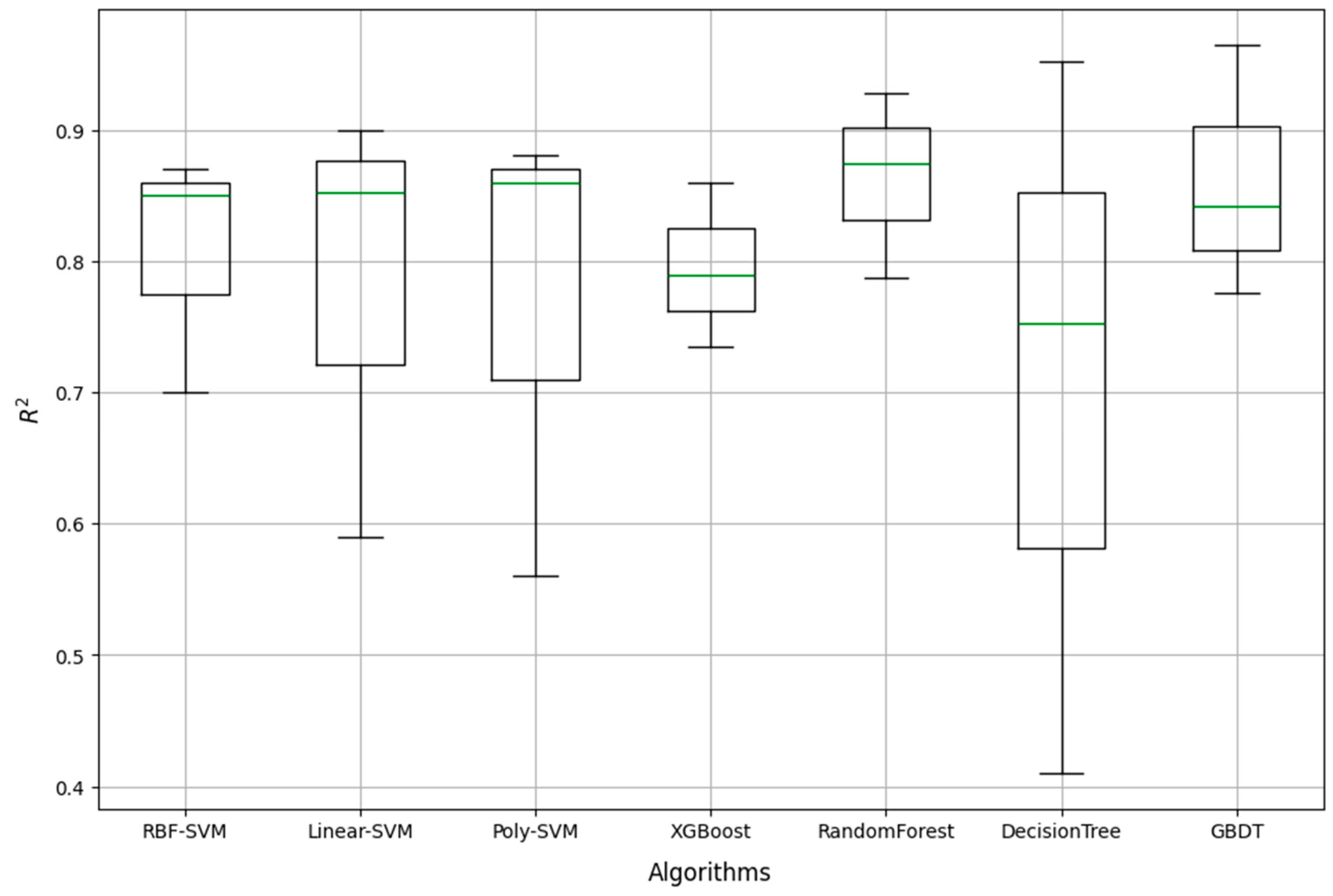
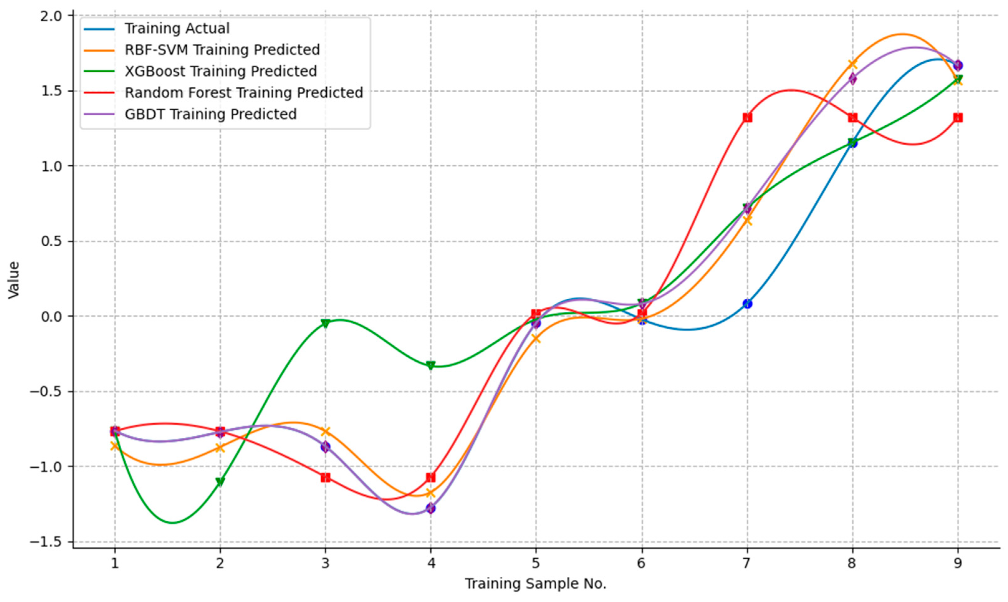
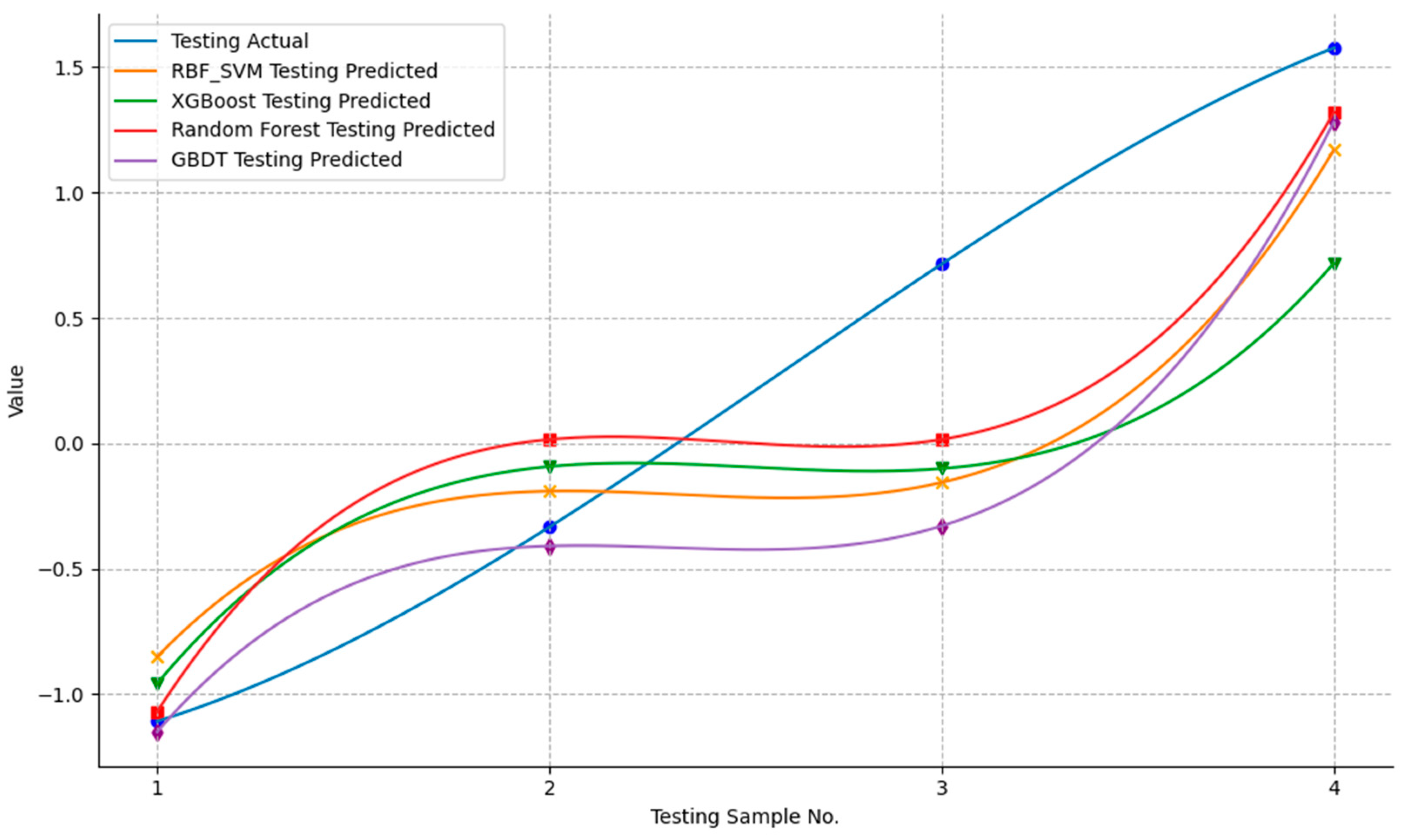
4.4.1. Model Comparison

After the models were established, their fitting performance on the training set and predictive performance on the test set were compared. The model comparisons are presented in Figure 2 and Figure 3.

The figures above show that on the test set, Model_rs and Model_gb exhibit relatively similar and good fitting performance, followed by Model_rf, while Model_xg performs poorly. On the training set, the prediction results of Model_rs, Model_rf, and Model_gb are significantly better than those of Model_xg. Overall, Model_rs and Model_gb achieved superior prediction results.

4.4.2. Evaluation Metrics

This paper utilizes four of the most commonly used metrics from the literature [15,16] to evaluate the performance of Model_rs, Model_xg, Model_rf, and Model_gb. These metrics include Mean Squared Error (MSE), Mean Absolute Error (MAE), Coefficient of Determination (R²), and Mean Absolute Percentage Error (MAPE). The MSE value ranges from 0 to infinity, where values closer to 0 indicate more stable predictions. The MAE value also ranges from 0 to infinity, where values closer to 0 indicate better model prediction performance. The R² value ranges from 0 to 1. On the training set, values closer to 1 indicate a better goodness of fit; on the test set, values closer to 1 indicate superior prediction performance. MAPEs value closer to 0 indicate better prediction performance. Typically, MAPE ≤ 10% indicates “high accuracy”, 10% < MAPE ≤ 20% indicates “good accuracy”, 20% < MAPE ≤ 50% indicates “reasonable accuracy”, and MAPE > 50% indicates “inaccuracy” [7]. The formulas for these metrics are presented in Equations (4)–(7).

$$MSE={\displaystyle \frac{1}{n}}{\displaystyle \sum _{i=1}^n{\left({\stackrel{⌢}{y}}_i-y_i\right)}^2}$$

(4)

$$MAE={\displaystyle \frac{1}{n}}{\displaystyle \sum _{i=1}^n\left|{\stackrel{⌢}{y}}_i-y_i\right|}$$

(5)

$$R^2=1-{\displaystyle \frac{{\displaystyle \sum _{i=1}^n{\left({\stackrel{⌢}{y}}_i-y_i\right)}^2}}{{\displaystyle \sum _{i=1}^n{\left({\overline{y}}_i-y_i\right)}^2}}}$$

(6)

$$MAPE={\displaystyle \frac{100\%}{n}}{\displaystyle \sum _{i=1}^n\left|\frac{{\widehat{y}}_i-y_i}{y_i}\right|}$$

(7)

where, $n$ represents the number of samples, i.e., the total number of samples in the dataset; $y_i$ represents the actual value of the $i$th sample, which is the true value in the dataset; $\stackrel{⌢}{y}i$ represents the predicted value of the $i$th sample, obtained from the model prediction; and $\overline{y}i$ represents the mean value of the $i$th sample.

4.4.3. Model Evaluation Results

After establishing the models, the MSE, MAE, R², and MAPE were calculated for each model on the test set. The average values of these metrics are used as evaluation indicators for the predictive models. The evaluation results for each model can be found in

Table 10. Evaluation results of the four models across four metrics.

Metric	Model
	Model_rs	Model_xg	Model_rf	Model_gb
MSE	0.0629	0.1301	0.0821	0.0754
MAE	0.2117	0.2577	0.2182	0.2002
R2	0.9350	0.8020	0.9134	0.9118
MAPE	1.0427	1.8969	1.0942	1.2280

.

Based on the results, it can be seen that Model_rs has the smallest MSE, indicating the best prediction stability. The MSE values of Model_rf and Model_gb are quite close, both yielding good results, and all three models significantly outperform Model_xg. Model_gb achieved the lowest MAE value, indicating the best prediction performance. The MAE values of Model_gb, Model_rs, and Model_rf are similar, while Model_xg has the highest MAE value, indicating a relatively poor prediction performance compared to the other three models. The R² values of Model_rs, Model_rf, and Model_gb all exceed 0.91, indicating that these models demonstrate superior predictive performance for Tibet’s transportation carbon emissions, with Model_rs demonstrating the best results. In contrast, Model_xg’s R² value of 0.8020 indicates it is less suitable for predicting Tibet’s transportation carbon emissions compared to the other three models. All four models have MAPE values below 10%, indicating high accuracy. Although Model_xg has a higher MAPE value, it remains below 10%. Considering all four metrics, Model_rs demonstrates superior prediction performance.

In summary, based on the presented analysis, the RBF-SVM algorithm is the most suitable for constructing a prediction model for Tibet’s transportation carbon emissions for the dataset in this paper. This finding aligns with the research results of Song et al. [37]. Therefore, the RBF-SVM algorithm is selected for subsequent research and analysis in this paper. The Random Forest and GBDT algorithms also performed well on this dataset and are suitable for constructing a prediction model for Tibet’s transportation carbon emissions, whereas the performance of the XGBoost algorithm requires improvement.

4.5. Model Improvement

4.5.1. Initial Selection of Improved Model

The dataset in this paper includes numerous input variables, potentially causing multicollinearity. Removing one or more variables could destabilize the explanatory model, leading to inaccurate results. Therefore, Partial Least Squares (PLS) is applied to decompose and reconstruct the input variables. PLS decomposes all 14 variables, extracts key components, and forms new independent principal components, thus mitigating the adverse effects of multicollinearity during modeling.

Accurate prediction with the RBF-SVM algorithm depends on adjusting two parameters: the regularization parameter and the kernel function coefficient. Common optimization algorithms for identifying optimal prediction model parameters include GS [16], Genetic Algorithm (GA), and Ant Colony Optimization (ACO) [15]. Therefore, this paper uses the deviation between predicted and actual values on the test set as the objective function, optimizing the regularization parameter and kernel function coefficient in the RBF-SVM algorithm. Using Python, the parameters of the model are optimized based on GS, Real-coded Genetic Algorithm (RGA), and ACO. To avoid errors due to randomness, ten repetitions of three-fold cross-validation are conducted, with the average R² value on the test set used as the evaluation metric. If the R² value does not increase significantly with the number of components, the corresponding number of components is considered optimal. The R² values of the optimized models across different principal components are presented in Figure 4.

As shown in Figure 4, the R² value of the ACO-optimized model is unstable, indicating a lack of model stability. The GS-optimized and RGA-optimized models both show a clear upward trend, with R² values stabilizing after the fifth principal component, indicating that the original model is effectively explained at this point. Therefore, this paper selects five principal components (denoted as $U_1$, $U_2$, $U_3$, $U_4$, $U_5$) for subsequent modeling. The formulas for the principal components are presented in Equations (8)–(12).

$$\begin{array}{l}{U}_1=0.0821x_1+0.663x_2+0.0804x_3+0.0563x_4+0.0247x_5+0.0778x_6+0.0811x_7\\ +0.0803x_8+0.0637x_9+0.0810x_{10}+0.0747x_{11}+0.0809x_{12}+0.0771c_1+0.0793c_2\end{array}$$

(8)

$$\begin{array}{l}{U}_2=0.1282x_1+0.1772x_2+0.1097x_3-0.0281x_4+0.1086x_5+0.0802x_6+0.1012x_7\\ +0.0859x_8-0.0266x_9+0.0996x_{10}+0.0366x_{11}+0.0934x_{12}+0.0960c_1+0.1007c_2\end{array}$$

(9)

$$\begin{array}{l}{U}_3=0.1281x_1+0.2136x_2+0.0503x_3+0.0918x_4+0.0776x_5+0.0863x_6+0.0673x_7\\ +0.0373x_8-0.3285x_9+0.0753x_{10}-0.1262x_{11}+0.0868x_{12}+0.2667c_1+0.4100c_2\end{array}$$

(10)

$$\begin{array}{l}{U}_4=0.1341x_1+0.2944x_2-0.0053x_3+0.0769x_4+0.0131x_5+0.0515x_6+0.0448x_7\\ +0.0083x_8-0.3690x_9+0.0771x_{10}-0.1664x_{11}+0.0897x_{12}+0.2653c_1+0.5457c_2\end{array}$$

(11)

$$\begin{array}{l}{U}_5=0.1098x_1+0.3189x_2-0.1449x_3+0.0470x_4+0.0797x_5+0.0289x_6+0.0106x_7\\ -0.0482x_8-0.3046x_9+0.0653x_{10}-0.1922x_{11}+0.0929x_{12}+0.2814c_1+0.8244c_2\end{array}$$

(12)

The coefficients of these five principal components are distinct and uncorrelated with each other. Thus, we transformed the fourteen correlated variables into five independent variables, reducing the dimensionality of the data. These five new variables were then used for model selection in Section 4.5.2.

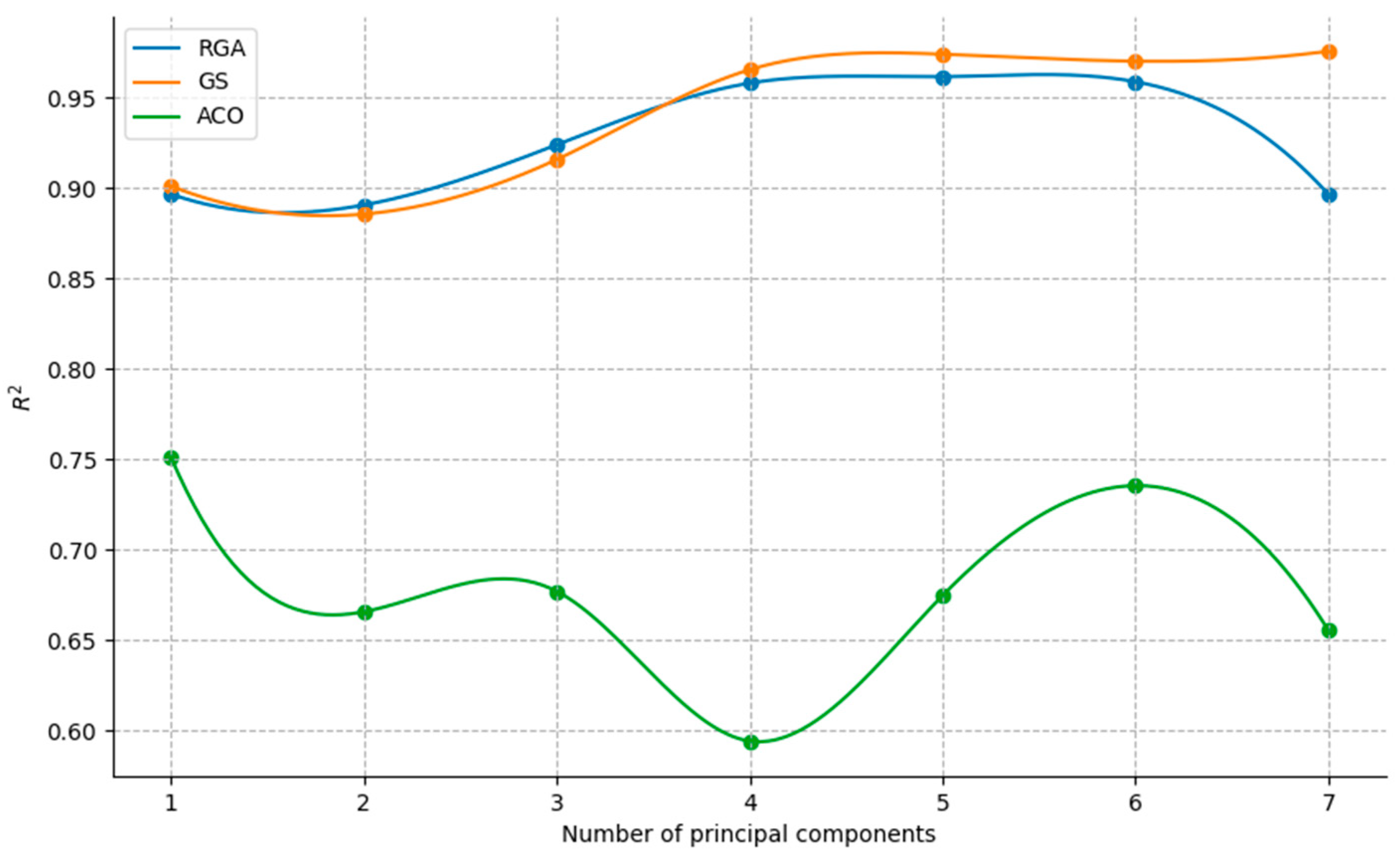
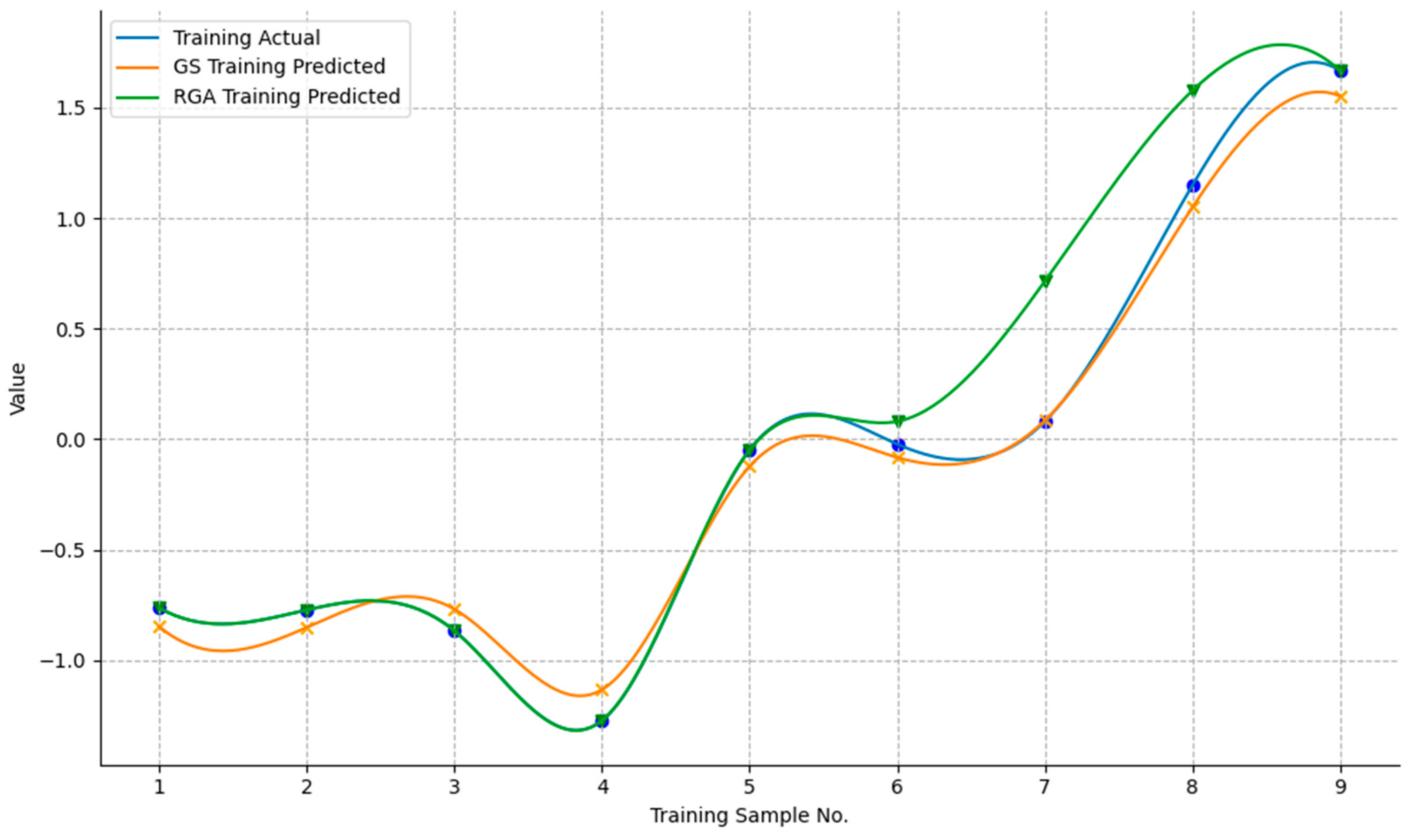
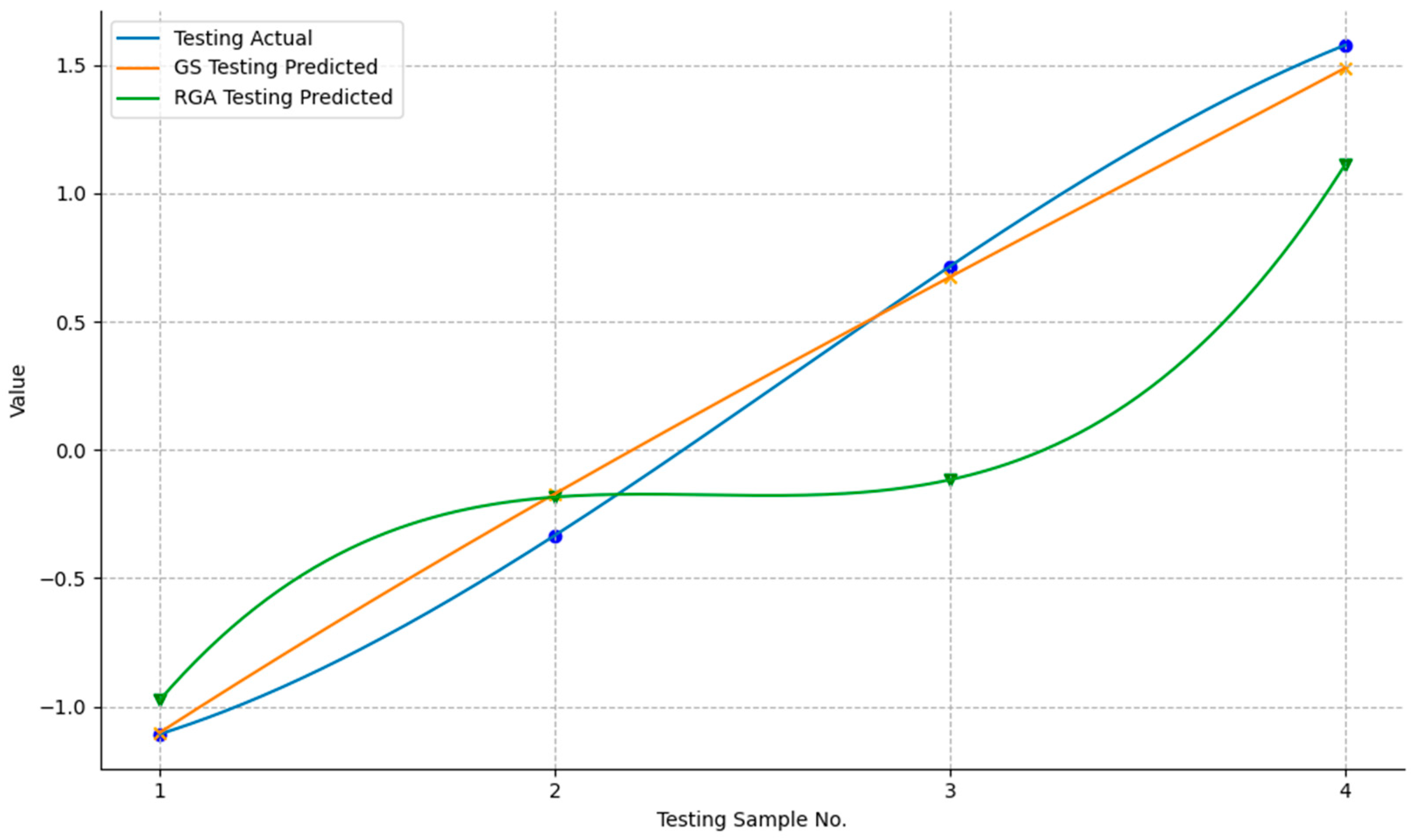
4.5.2. Final Selection of the Improved Model

As discussed in Section 4.5.1, both GS and RGA showed good results in the initial optimization of model parameters. This paper further utilizes these two algorithms to optimize the RBF-SVM model, establishing Model_gs_rs and Model_rga_rs.

Grid Search systematically traverses predefined combinations of hyperparameters to identify the best model parameters [38]. The basic process is as follows:

• Step 1. Parameter Grid: Set the parameters to be searched and their value ranges.
• Step 2. Model Training and Validation: Train the model and perform cross-validation for each parameter combination in the grid.
• Step 3. Select Best Parameters: Select the parameter combination with the best performance based on cross-validation metrics.

Real-coded Genetic Algorithm is an optimization algorithm that simulates natural selection and genetic mechanisms. Unlike traditional binary-coded genetic algorithms, RGA employs real number encoding, making it more effective for continuous variable optimization [39]. The basic process is as follows:

• Step 1. Initialization: Randomly generate a set of real-number candidate solutions.
• Step 2. Fitness Evaluation: Evaluate the quality of each candidate solution using a predefined fitness function.
• Step 3. Selection: Apply a fitness-based selection strategy to choose superior candidate solutions as parents for the next generation.
• Step 4. Crossover: Generate new candidate solutions by exchanging parts of the variables between parent solutions.
• Step 5. Mutation: Randomly modify the genes of some candidate solutions to enhance diversity.
• Step 6. Replacement: Replace the old generation with the new generation and iterate until the termination condition is met.

The data from 2008 to 2020, after extracting five principal components, were used for model construction with three-fold cross-validation. The parameters selected for the optimization algorithms of the two models and the optimized RBF-SVM parameters can be found in

Table 11. Parameters for the optimization algorithms in Model_gs_rs and Model_rga_rs, along with the optimized RBF-SVM parameters.

Model	Python Library	Optimization Algorithm Parameters	RBF-SVM Parameters
Model_gs_rs	Machine learning library: Scikit-learn	Regularization parameter: [0.01, 0.1, 1, 10, 100, 1000] Kernel coefficient: [0.0001, 0.001, 0.01, 0.1, 1]	Regularization Parameter: 1000 Kernel coefficient: 0.001
Model_rga_rs	Machine learning library: Scikit-learn and DEAP	Selection: Grid Search Crossover: Uniform Crossover Fitness function: Evaluate Population size: 50 Generations: 40+ Crossover rate: 0.5 Mutation rate: 0.2	Regularization Parameter: 42.76 Kernel coefficient: 0.02

.

The four metrics from Section 4.4.2.—MSE, MAE, R², and MAPE—are employed to evaluate Model_gs_rs and Model_rga_rs. The prediction performance of each model is presented in Figure 5 and Figure 6, and the accuracy comparison of the models can be found in

Table 12. Evaluation results of each optimized model across four metrics.

Metric	Model
	Model_gs_rs	Model_rga_rs
MSE	0.0089	0.0220
MAE	0.0907	0.1200
R2	0.9924	0.9835
MAPE	0.2990	0.1198

.

The figures above show that on the test set, Model_rga_rs has a better fitting effect in the first half, while in the second half, Model_gs_rs achieves better results, with Model_rga_rs showing larger deviations. Overall, Model_gs_rs demonstrates a better fitting effect on the test set. On the training set, the prediction results of Model_gs_rs are significantly better than those of Model_rga_rs. In summary, the GS optimization of the RBF-SVM algorithm yields better results compared to RGA.

The table shows that Model_gs_rs has a smaller MSE value than Model_rga_rs, indicating better prediction stability. The MAE value of Model_gs_rs is also lower, reflecting superior prediction performance. The R² value of Model_gs_rs exceeds 0.99, achieving an ideal prediction result for Tibet’s transportation carbon emissions, while Model_rga_rs also performs well with an R² value above 0.98. Both models have MAPE values below 10%, indicating high prediction accuracy. Overall, Model_gs_rs demonstrates the best prediction performance. Therefore, after applying PLS, the RBF-SVM algorithm optimized by GS is identified as the most suitable for constructing a prediction model for Tibet’s transportation carbon emissions with this dataset, making Model_gs_rs the preferred choice for further research and analysis.

5. Analyzing the Contribution of Variables to Model Output

5.1. Local Sensitivity Analysis

Local sensitivity analysis evaluates the impact of individual variables on model output by applying small perturbations to the input variables and observing the resulting output changes [40]. The finite difference method approximates the derivative using a finite difference expression (Equation (14)) based on the derivative definition (Equation (13)). Perturbing input variables slightly and observing output changes, the model’s sensitivity to each variable can be estimated [41]. There are three types of finite difference methods: forward difference, backward difference, and central difference. Central difference, which accounts for changes around the point x, is typically more accurate than forward or backward difference. Thus, the central difference method is used in this section, with its formula presented in Equation (15).

$$f^{\prime }\left(x\right)\approx \underset{\Delta x\to 0}{\lim }{\displaystyle \frac{f\left(x+\Delta x\right)-f\left(x\right)}{\Delta x}}$$

(13)

In practical applications, a very small number $h$ is used to approximate $\Delta x$, leading to a finite difference approximation:

$$f^{\prime }\left(x\right)\approx {\displaystyle \frac{f\left(x+h\right)-f\left(x\right)}{h}}$$

(14)

$$S_i={\displaystyle \frac{f\left(x_1,x_2,x_3,\dots x_i+h,\dots x_n\right)}{2h}}$$

(15)

To evaluate the impact of the 12 core variables on the model output, a local sensitivity analysis is performed on Model_gs_rs using the central difference method. Each core variable is perturbed with a step size of 0.00001, and the resulting changes are input into the model to observe their effect on the final output. The impact of each variable on the model output is presented in Figure 7.

In the figure, each bar corresponds to a variable, where darker colors signify a greater influence on the model output. The variables are ranked in descending order of their impact on the model output as follows: $x2$, $x9$, $x11$ $x3$, $x1$, $x12$, $x10$, $x4$, $x5$, $x8$, $x6$, and $x7$.

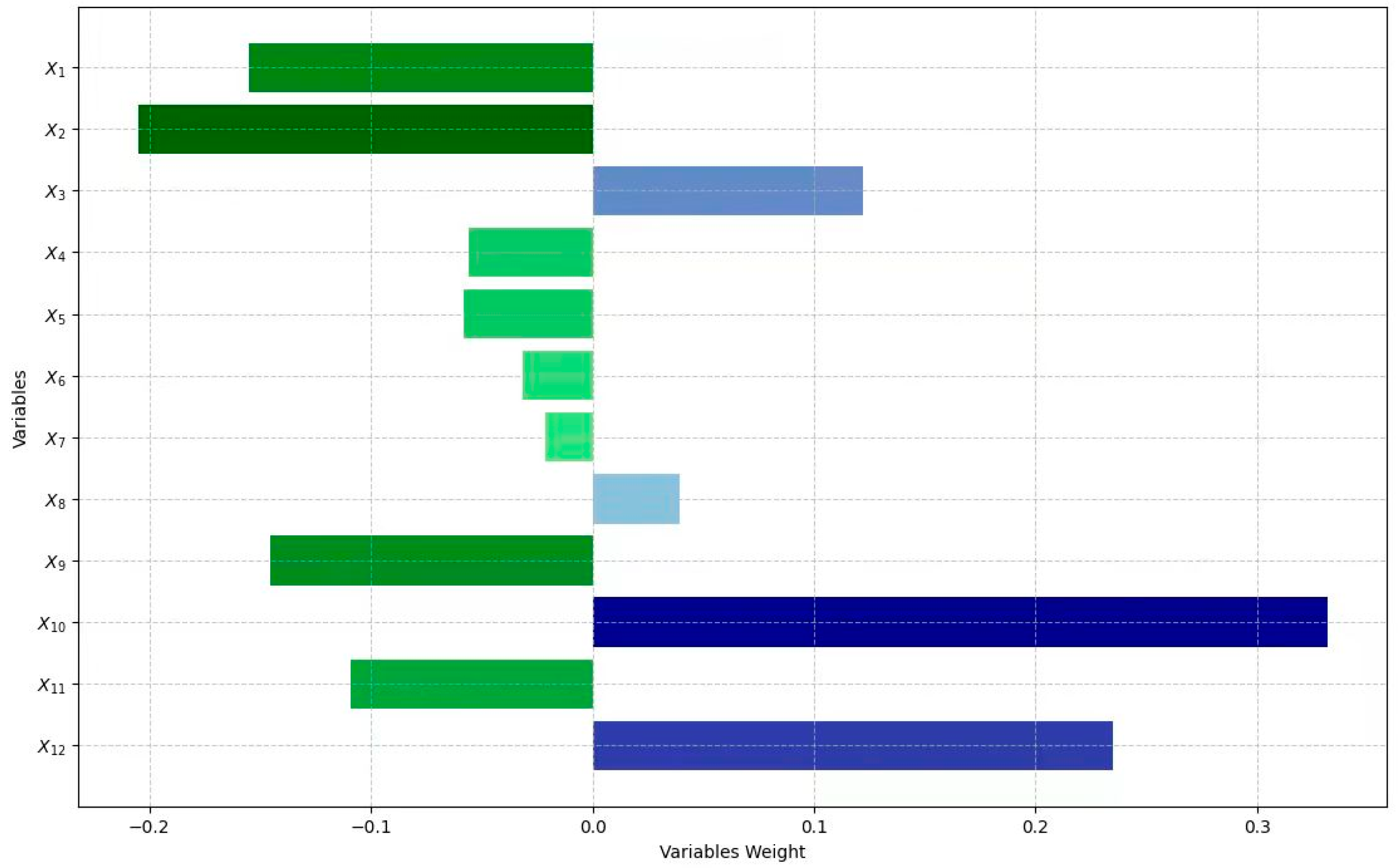
5.2. Interpretability Analysis

There are many classifications of interpretability methods, including those based on applicable models, based on timing, and based on individual and global perspectives. This paper focuses on using post-hoc interpretability methods to explain the model. LIME (Local Interpretable Model-Agnostic Explanation) is a model-agnostic local surrogate model used to explain the predictions of black-box models [42]. The concept behind LIME is straightforward: train a local surrogate model to explain each prediction. The process works as follows:

• Step 1. Generate multiple perturbed samples around the data point to be explained.
• Step 2. Use the original model to predict these perturbed samples.
• Step 3. Train an interpretable model using these perturbed samples and their prediction results.
• Step 4. The coefficients of the surrogate model indicate the importance of each feature to the original model’s prediction.

To obtain interpretable model parameters, an objective function for optimization must be constructed for the algorithm. The objective function of the LIME algorithm is presented in Equation (16).

$$\xi \left(x\right)=\underset{g\in G}{\arg \min }L\left(f,g,{\prod }_x\right)+\Omega \left(x\right)$$

(16)

where $f$ represents the complex model that needs to be explained; $G$ represents the potential interpretable model, such as a linear model, Decision Tree, etc.; $g$ represents the interpretable simple model; $x$ represents the example data; ${\prod }_x$ represents the proximity of the example data to the perturbed data; $L\left(f,g,{\prod }_x\right)$ represents the degree of local unfaithfulness of the model; and $\Omega \left(x\right)$ represents the complexity of the model $g$.

In this section, Model_gs_rs is the complex model being explained, and a linear regression model is selected as the interpretable simple model. Twelve core variables were analyzed using the LIME algorithm to assess their impact on Model_gs_rs. The analysis was conducted using Python programming, and all other parameters and configurations were left at their default settings in Python. The results of the interpretability analysis based on the LIME algorithm are presented in Figure 8.

In the figure, each bar represents a variable, with blue indicating a positive correlation (+) with carbon emissions and green indicating a negative correlation (−). Darker colors denote stronger correlations. The variables are ranked by importance from highest to lowest as follows: $x10$ (+), $x12$ (+), $x2$ (−), $x1$ (−), $x9$ (−), $x3$ (+), $x11$ (−), $x5$ (−), $x4$ (−), $x8$ (+), $x6$ (−), and $x7$ (−).

Based on the feature importance analysis and the sensitivity analysis, variables $x4$ through $x8$ have a smaller contribution to the model output. This indicates that total public transport passenger volume, the number of buses and electric vehicles per 10,000 people, tourism revenue, and the number of tourists have less impact on Tibet’s transportation carbon emissions. Conversely, variables $x1$ through $x3$ and $x9$ through $x12$ make a more significant contribution to the model output, indicating that number of civilian vehicles, transportation land-use area, transportation output value, urban green coverage areas, per capita GDP, and built-up area have a greater impact on carbon emissions. Additionally, transportation output value, total retail sales of consumer goods, urban green coverage areas, and built-up area positively impact carbon emissions, whereas the remaining variables have a negative impact. From a dimensional perspective, the level of transportation and socio-economic development have a greater influence on carbon emissions.

6. Discussion on Variables Affecting Transportation Carbon Emissions

6.1. Transportation Development Level

The transportation development significantly impacts carbon emissions in Tibet, making it a crucial dimension directly influencing these emissions. The corresponding factors, including transportation land-use area, transportation output value, and the number of civilian vehicles, all strongly influence carbon emissions in Tibet’s transportation sector. The transportation land-use area has a significant impact on reducing carbon emissions. A larger transportation land area can provide more roads and transportation facilities, optimize the transportation network, reduce traffic congestion [43], and consequently lower carbon emissions. The number of civilian vehicles also has a significant impact on reducing carbon emissions. There is an inverted “U” relationship between the number of civilian vehicles and carbon emissions. When the number of civilian vehicles reaches a high level, low-carbon vehicles, such as hybrid and electric vehicles gradually dominate the market. As low- or zero-emission vehicles become more prevalent, overall carbon emissions decrease, despite an increase in vehicle numbers, because these vehicles emit significantly less carbon than traditional internal combustion engine vehicles [20]. In recent years, the rate of electric vehicle purchases in Tibet has grown significantly, outpacing that of gasoline vehicles. Low-carbon vehicles now dominate the market [44], contributing to the descending segment of the inverted “U” curve in Tibet’s transportation carbon emissions. Furthermore, the rapid increase in civilian vehicles has prompted the government and relevant departments to improve transportation infrastructure, including more efficient road systems and optimized traffic signals. These measures have reduced congestion, improved vehicle efficiency [45], and thus lowered fuel consumption and carbon emissions. The transportation output value has a certain impact on promoting carbon emissions in Tibet’s transportation sector. The transportation industry’s output value directly reflects the development level of the sector. An increase in output value is often accompanied by higher energy consumption, as frequent and intensive transportation activities lead to more fuel use [46], thereby increasing carbon emissions.

6.2. Public Transportation Development Level

Although public transportation development in Tibet contributes to emission reductions, its impact is relatively small. The primary reason is Tibet’s slow economic development, leading to limited investment in public transportation, which remains insufficient to meet people’s travel needs [47]. Additionally, Tibet’s complex geography and scattered population make it difficult for public transit systems to cover extensive areas [48]. Consequently, public transportation in Tibet has not fulfilled its potential to reduce emissions.

6.3. Tourism Development Level

The development of tourism in Tibet has a relatively small impact on reducing transportation carbon emissions. Tibet’s tourism industry is highly seasonal, with peak periods in summer and autumn, and fewer visitors during other seasons. This seasonality causes uneven transportation carbon emissions throughout the year [49], with minimal impact on the annual total emissions. Additionally, the development of Tibet’s tourism has optimized transportation resources and improved infrastructure, though these improvements are often limited to popular tourist areas [3]. Moreover, the number of tourists indirectly reflects those driving their own or rented vehicles [50]; thus, the carbon emissions from these activities contribute relatively little to the overall carbon emissions in Tibet. Consequently, tourism development has a relatively small impact on reducing transportation carbon emissions in Tibet.

6.4. Tertiary Industry Development Level

The development of the tertiary industry significantly impacts Tibet’s transportation carbon emissions, with its output value making a particularly notable contribution to emission reductions. The output value of the tertiary industry directly reflects the development level of Tibet’s tertiary sector. As information technology spreads in Tibet, many tertiary industry activities can be conducted remotely or online, reducing travel needs and thus lowering transportation carbon emissions [51]. The development of the retail industry generates substantial logistics and supply chain activity, leading to increased transportation carbon emissions.

6.5. Socio-Economic Development Level

Socio-economic development also has a significant impact on Tibet’s transportation carbon emissions, serving as a major dimension indirectly influencing these emissions. The urban green coverage and built-up areas within this dimension substantially reduce Tibet’s transportation carbon emissions. Both factors measure the level of urban development in Tibet and indirectly reflect social development. Larger green coverage and built-up areas in Tibet indicate higher urban development, which in turn improves people’s living standards and makes travel more convenient [52]. Additionally, increased green spaces enhance urban attractiveness, prompting more people to drive to these areas for recreation [53]. These factors contribute to higher transportation energy consumption and, consequently, increased carbon emissions. Per capita GDP has a certain impact on reducing carbon emissions, as it directly reflects the level of economic development. As Tibet’s economy grows, the proportion of the tertiary industry increases. Compared to industry and agriculture, the service sector has lower carbon intensity and relies more on information technology and remote work, reducing the need for travel and associated emissions. Furthermore, Tibet’s economic development has heightened public environmental awareness, increasing emphasis on conservation and encouraging more people to choose low-carbon travel methods [54].

7. Conclusions

This paper begins by refining the UNWTO’s transportation carbon emissions model, applying it to estimate Tibet’s transportation carbon emissions from 2008 to 2020 using transportation turnover data. Next, based on the literature review and considering the characteristics of Tibet, the dimensions and factors influencing Tibet’s carbon emissions were identified to create input variables and construct a prediction model for Tibet’s transportation carbon emissions. The model was then refined to identify the most suitable prediction algorithm. Following feature extraction using the PLS method, various parameter optimization techniques were applied to develop new models, with the most accurate and stable model being selected. Finally, sensitivity and interpretability analyses were conducted using the central difference method and LIME algorithm to assess the influence of each variable on the model output, allowing for a comprehensive analysis of their impact on Tibet’s transportation carbon emissions. The key findings of this paper are as follows:

(1)

The total carbon emissions from Tibet’s transportation sector show a significant upward trend. Notably, emissions from civil aviation passenger transport see the most dramatic rise, surging from 15.54 thousand tons in 2011 to 884.45 thousand tons in 2020, a 56.91-fold increase. Road freight remains the largest contributor, responsible for 62.29% of the transportation carbon emissions in Tibet.

(2)

The model construction reveals that the RBF-SVM algorithm is the most suitable for predicting Tibet’s transportation carbon emissions. After optimizing RBF-SVM using GS and RGA, the enhanced model (Model_gs_rs) achieves superior performance, with an R² value exceeding 0.99, significantly enhancing the prediction accuracy.

(3)

Regarding the impact on Tibet’s transportation carbon emissions, factors like total public transport passenger volume, the number of buses and electric vehicles per 10,000 people, tourism revenue, and the number of tourists have minimal influence. In contrast, the number of civilian vehicles, transportation land-use area, transportation output value, urban green coverage areas, per capita GDP, and built-up area exert a more significant impact. Dimensionally, the levels of transportation development and socio-economic development are the most critical determinants of carbon emissions.

The data used in this paper span a relatively short period, limiting the ability to fully capture long-term trends and shifts in Tibet’s transportation carbon emissions. To address this limitation, an extended data collection period should be employed in future research, allowing for a more comprehensive analysis of long-term changes. Additionally, although Chinese transportation carbon emission factors were used to estimate emissions in Tibet, factors such as altitude and environmental conditions could introduce potential estimation errors. Moreover, interpolation issues may arise due to large gaps in carbon emission factor data. This is particularly true when using cubic spline interpolation for certain years, which could result in inaccuracies when trends are complex or nonlinear. To minimize these interpolation uncertainties, more continuous and detailed carbon emission factor data should be collected in future studies. Finally, although traditional machine learning algorithms, which involve complex parameter optimization and high computational demand, were primarily used in this paper, future research could benefit from exploring more advanced and efficient prediction models, such as deep learning algorithms. These models offer better prediction accuracy and computational efficiency, thus enhancing both model performance and resource optimization.

References

1. Wang, S.; Ge, M. Everything You Need to Know about the Fastest-Growing Source of Global Emissions: Transport. World Resources Institute 16 October 2019. Available online: https://www.wri.org/insights/everything-you-need-know-about-fastest-growing-source-global-emissions-transport#:~:text=1.%20How%20big%20a%20problem%20are%20emissions%20from (accessed on 18 October 2023).
2. Jelti, F.; Allouhi, A.; Tabet Aoul, K.A. Transition Paths towards a Sustainable Transportation System: A Literature Review. Sustainability 2023, 15, 15457. [Google Scholar] [CrossRef]
3. Wang, J.; Yi, L.; Chen, L.; Hou, Y.; Zhang, Q.; Yang, X. Coupling and Coordination between Tourism, the Environment and Carbon Emissions in the Tibetan Plateau. Sustainability 2024, 16, 3657. [Google Scholar] [CrossRef]
4. World Tourism Organization; United Nations Environment Programme. Climate Change and Tourism: Responding to Global Challenges; World Tourism Organization: Madrid, Spain, 2008; pp. 139–143. [Google Scholar]
5. Cai, B.; Yang, W.; Cao, D.; Liu, L.; Zhou, Y.; Zhang, Z. Estimates of China’s National and Regional Transport Sector CO2, Emissions in 2007. Energy Policy 2012, 41, 474–483. [Google Scholar] [CrossRef]
6. Zhu, C.; Wang, M.; Du, W. Prediction on peak values of carbon dioxide emissions from the Chinese transportation industry based on the SVR model and scenario analysis. J. Adv. Transp. 2020, 2020, 8848149. [Google Scholar] [CrossRef]
7. Ağbulut, Ü. Forecasting of transportation-related energy demand and CO2 emissions in Turkey with different machine learning algorithms. Sustain. Prod. Consum. 2022, 1, 141–157. [Google Scholar] [CrossRef]
8. Ma, S.; Chen, X.; Yang, L.; Zhao, Y.; Zeng, Y. Impacts of Accessibility on Sspatial Heterogeneity of Multimodal Transportation Carbon Emissions in an Urban Agglomeration. J. Transp. Syst. Eng. Inf. Technol. 2024, 24, 64–74. [Google Scholar]
9. Gao, J.; Huang, W.; Jiang, H. Comparison of Multiple Forecast Models of Urban Traffic Carbon Emissions. J. Chongqing Jiaotong Univ. (Nat. Sci.) 2020, 39, 33–39. [Google Scholar]
10. Li, N.; Chen, S.; Liang, X.; Tian, P. Prediction of Transportation Industry Carbon Peak in China. J. Transp. Syst. Eng. Inf. Technol. 2024, 24, 2–13+54. [Google Scholar]
11. Jiao, L.; Liu, Y.; Wu, Y.; Huo, X. Transportation Carbon Emission Prediction Based on Convolutional Neural Network. Railw. Transp. Econ. 2024, 1–9. [Google Scholar]
12. Zhao, J.; Li, J.; Wang, P.; Hou, G. A Study on Carbon Peaking Paths in Henan, China Based on Lasso Regression-BP Neural Network Model. Environ. Eng. 2022, 40, 151–156+164. [Google Scholar]
13. Wei, S.; Wang, Y.; Zhang, C. Forecasting CO2 emissions in Hebei, China, through moth-flame optimization based on the random forest and extreme learning machine. Environ. Sci. Pollut. Res. 2018, 25, 28985–28997. [Google Scholar] [CrossRef] [PubMed]
14. Wang, Q.; Wang, J.; Zhu, C.; Hao, F. Carbon Emission Prediction of Transportation Industry Based on VMD and SSA-LSSVM. Environ. Eng. 2023, 41, 124–132. [Google Scholar]
15. Huo, Z.; Zha, X.; Lu, M.; Ma, T.; Lu, Z. Prediction of carbon emission of the transportation sector in Jiangsu province-regression prediction model based on GA-SVM. Sustainability 2023, 15, 3631. [Google Scholar] [CrossRef]
16. Liu, H.; Hu, D. Construction and Analysis of Machine Learning Based Transportation Carbon Emission Prediction Model. Environ. Eng. 2024, 45, 3421–3432. [Google Scholar]
17. Zhao, G.; Gao, Y.; Wang, Z. A Transportation Carbon Emission Analysis Method Based on Decision Tree and Monte Carlo Simulation. Highway 2015, 60, 191–195. (In Chinese) [Google Scholar]
18. Jiang, Y.; Zhou, Z.; Liu, C. The impact of public transportation on carbon emissions: A panel quantile analysis based on Chinese provincial data. Environ. Sci. Pollut. Res. 2019, 26, 4000–4012. [Google Scholar] [CrossRef] [PubMed]
19. Wang, J.; Yan, Y.; Huang, Q.; Song, Y. Analysis of Carbon Emission Reduction Potential of China’s Transportation. Sci. Technol. Manag. Res. 2021, 41, 200–210. [Google Scholar]
20. Hou, L.; Wang, Y.; Zheng, Y.; Zhang, A. The Impact of Vehicle Ownership on Carbon Emissions in the Transportation Sector. Sustainability 2022, 14, 12657. [Google Scholar] [CrossRef]
21. Hussain, Z.; Khan, M.K.; Shaheen, W.A. Effect of economic development, income inequality, transportation, and environmental expenditures on transport emissions: Evidence from OECD countries. Environ. Sci. Pollut. Res. 2022, 29, 56642–56657. [Google Scholar] [CrossRef]
22. Tian, P.; Mao, B.; Tong, R.; Zhang, H.; Zhou, Q. Analysis of carbon emission level and intensity of China’s transportation industry and different transportation modes. Clim. Change Res. 2023, 19, 347–356. [Google Scholar]
23. Wang, Z.; Li, J.; Peng, B.; Xiang, W. Driving Factors and Decoupling Effect Analysis of Transportation Carbon Emissions in Western China. Environ. Eng. 2023, 41, 213–222. [Google Scholar]
24. Wang, C.; Wu, L. Factors Driving the Carbon Emission Reduction in Transport Along the Silk Road Economic Belt: An Analysis from the Perspective of “Double Carbon”. J. Arid Land Resour. Environ. 2024, 38, 9–19. [Google Scholar]
25. Liu, J.; Liu, Y.; Huang, L. Measurement and Driving Factor Analysis of Carbon Emissions from Tourism Transportation in East China. Res. Environ. Sci. 2024, 37, 626–636. [Google Scholar]
26. Li, J.; Li, M.; Yuan, M.; Li, M. Study on the Spatial and Temporal Evolution and Influencing Factors of Tourism Traffic Carbon Emissions in Provinces along the Grand Canal Cultural Belt. Ecol. Econ. 2024, 40, 145–152+173. [Google Scholar]
27. He, M.; Xie, J.; Wu, X.; Luo, J. Factors Decomposition of Carbon Emissions from Transportation Energy Consumption in Jiangsu Province Based on LMDI. Math. Pract. Theory 2015, 45, 16–22. [Google Scholar]
28. Bian, L.; Ji, M. Research on Influencing Factors and Prediction of Transportation Carbon Emissions in Qinghai. Ecol. Econ. 2019, 35, 35–39+100. [Google Scholar]
29. Liu, X.; Wu, P.; Wang, H. Analysis of Driving Factors of Transport Carbon Emissions in Inner Mongolia Based on LMDI Model. Transp. Energy Conserv. Environ. Prot. 2024, 20, 89–93+100. [Google Scholar]
30. Huang, L.; Liu, J.; Liu, Y.; Ju, X.; Wang, P. Spatial and temporal evolution characteristics and driving factors of urban traffic carbon emissions in Jiangsu Province. Environ. Ecol. 2024, 6, 1–8. [Google Scholar]
31. Liu, Y.; Wu, M.; Mu, R. Carbon Emission Measurement, Factor Decomposition and Low Carbonization Strategies of Transportation Industry in Tibet. J. Tibet Univ. 2021, 36, 126–133. [Google Scholar]
32. Gong, J.; Hu, J.; Wang, X. Analysis of the Influencing Factors of Carbon Emissions from Urban Transportation. Automob. Technol. 2024, 49, 170–174. [Google Scholar]
33. Eggleston, S.; Buendia, L.; Miwa, K.; Ngara, T.; Tanabe, K. 2006 IPCC Guidelines for National Greenhouse Gas Inventories; Institute for Global Environmental Strategies: Hayama, Japan, 2006. [Google Scholar]
34. Su, X.; An, J.; Zhang, Y. Support vector machine regression forecasting of O3 concentrations based on wavelet transformation. China Environ. Sci. 2019, 39, 3719–3726. [Google Scholar]
35. Zhao, N.; Lu, Y. Remote-sensing estimation of near-surface ozone concentration based on XGBoost. Acta Sci. Circumstantiae 2022, 42, 95–108. [Google Scholar]
36. Montes, C.; Kapelan, Z.; Saldarriaga, J. Predicting non-deposition sediment transport in sewer pipes using Random forest. Water Res. 2021, 189, 116639. [Google Scholar] [CrossRef] [PubMed]
37. Song, Y.; Shu, Q.; Jin, C.; Zheng, S.; Luo, L. Regional Transport Carbon Emission Forecasting and Peak Carbon Pathway Planning in China. Environ. Sci. 2024, 1–18. [Google Scholar] [CrossRef]
38. Shekar, B.H.; Dagnew, G. Grid Search-Based Hyperparameter Tuning and Classification of Microarray Cancer Data. In Proceedings of the 2019 Second International Conference on Advanced Computational and Communication Paradigms (ICACCP), Majitar, East Sikkim, India, 25–28 February 2019; pp. 1–8. [Google Scholar]
39. Alibrahim, H.; Ludwig, S.A. Hyperparameter optimization: Comparing genetic algorithm against grid search and bayesian optimization. In Proceedings of the 2021 IEEE Congress on Evolutionary Computation (CEC), Krakow, Poland, 28 June–1 July 2021; pp. 1551–1559. [Google Scholar]
40. Gustafson, P.; Srinivasan, C.; Wasserman, L. Local sensitivity analysis. Bayesian Stat. 1996, 5, 197–210. [Google Scholar]
41. Tortorelli, D.A.; Michaleris, P. Design sensitivity analysis: Overview and review. Inverse Probl. Eng. 1994, 1, 71–105. [Google Scholar] [CrossRef]
42. Ribeiro, M.T.; Singh, S.; Guestrin, C. “Why should i trust you?” Explaining the predictions of any classifier. In Proceedings of the 22nd ACM SIGKDD International Conference on Knowledge Discovery and Data Mining, San Francisco, CA, USA, 13–17 August 2016; pp. 1135–1144. [Google Scholar]
43. Bao, Z.; Ou, Y.; Chen, S.; Wang, T. Land use impacts on traffic congestion patterns: A tale of a Northwestern Chinese City. Land 2022, 11, 2295. [Google Scholar] [CrossRef]
44. Palden, N.; Da, Q. Electric Vehicle Sales Increase in Tibet as Infrastructure Expanded. The China Daily Global, 18 October 2023. Available online: https://usa.chinadaily.com.cn/a/202310/18/WS652f1cefa31090682a5e91a0.html (accessed on 18 October 2023).
45. Li, H.; Luo, N. Will improvements in transportation infrastructure help reduce urban carbon emissions?—Motor vehicles as transmission channels. Environ. Sci. Pollut. Res. 2022, 29, 38175–38185. [Google Scholar] [CrossRef]
46. Zhang, Y.; Kong, Y.; Quan, J.; Wang, Q.; Zhang, Y.; Zhang, Y. Scenario analysis of energy consumption and related emissions in the transportation industry—A case study of Shaanxi Province. Environ. Sci. Pollut. Res. 2024, 31, 26052–26075. [Google Scholar] [CrossRef] [PubMed]
47. Yang, X.; Qiu, X.; Fang, Y.; Xu, Y.; Zhu, F. Spatial variation of the relationship between transport accessibility and the level of economic development in Qinghai-Tibet Plateau, China. J. Mt. Sci. 2019, 16, 1883–1900. [Google Scholar] [CrossRef]
48. Xu, J.; Liu, J.; Xu, Y.; Pei, T. Visualization and analysis of local and distant population flows on the Qinghai-Tibet Plateau using crowd-sourced data. J. Geogr. Sci. 2021, 31, 231–244. [Google Scholar] [CrossRef]
49. Sang, S.; He, W.; Ni, M. How off-season tourism promotion affects seasonal destinations? A multi-stakeholder perspective in Tibet. Tour. Rev. 2021, 76, 229–240. [Google Scholar]
50. Wang, B.; Yang, Z.; Han, F.; Shi, H. Car Tourism in Xinjiang: The Mediation Effect of Perceived Value and Tourist Satisfaction on the Relationship between Destination Image and Loyalty. Sustainability 2017, 9, 22. [Google Scholar] [CrossRef]
51. Zheng, Y.; Wang, S.; Liu, L.; Aloisi, J.; Zhao, J. Impacts of remote work on vehicle miles traveled and transit ridership in the USA. Nat. Cities 2024, 1, 346–358. [Google Scholar] [CrossRef]
52. Jabbar, M.; Yusoff, M.M.; Shafie, A. Assessing the role of urban green spaces for human well-being: A systematic review. GeoJournal 2022, 87, 4405–4423. [Google Scholar] [CrossRef] [PubMed]
53. Lombardía, A.; Gómez-Villarino, M.T. Green infrastructure in cities for the achievement of the un sustainable development goals: A systematic review. Urban Ecosyst. 2023, 26, 1693–1707. [Google Scholar] [CrossRef]
54. Ma, H.; Chen, W.; Ma, H.; Yang, H. Influence of publicity and education and environmental values on the green consumption behavior of urban residents in Tibet. Int. J. Environ. Res. Public Health 2021, 18, 10808. [Google Scholar] [CrossRef]
Figure 1. R2 scores of each model from three-fold cross-validation.
Sustainability 16 08419 g001
Figure 2. Comparison of fitted values and actual values on the training set for the four models.
Sustainability 16 08419 g002
Figure 3. Comparison of predicted values and actual values on the test set for the four models.
Sustainability 16 08419 g003
Figure 4. R2 scores of the three optimized models across different principal components.
Sustainability 16 08419 g004
Figure 5. Comparison of fitted values and actual values on the training set for Model_gs_rs and Model_rga_rs.
Sustainability 16 08419 g005
Figure 6. Comparison of predicted values and actual values on the test set for Model_gs_rs and Model_rga_rs.
Sustainability 16 08419 g006
Figure 7. Impact of core variables on model output using the central difference method.
Sustainability 16 08419 g007
Figure 8. Feature importance of variables using LIME mean values.
Sustainability 16 08419 g008