
A Network-Constrained Integrated Method for Detecting Spatial Cluster and Risk Location of Traffic Crash: A Case Study from Wuhan, China


Abstract
:1. Introduction
2. Data and Methods
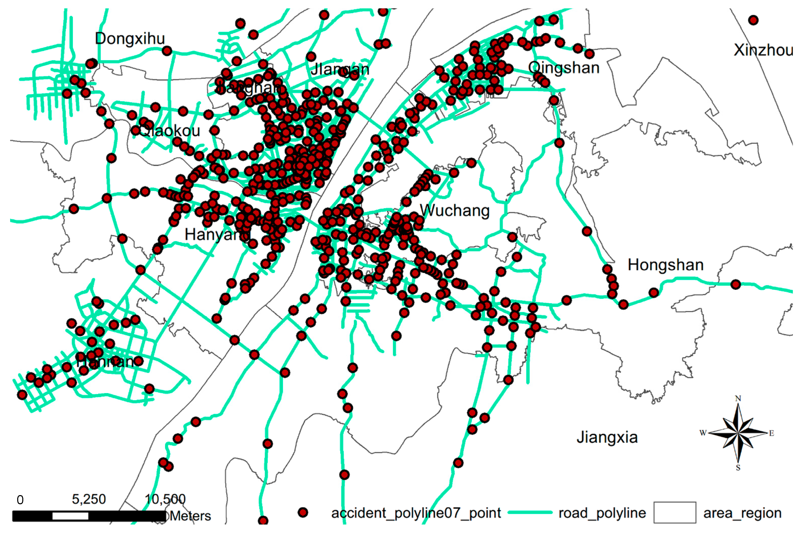
2.1. Data Source

2.2. Methods
2.2.1. Network Kernel Density Estimation
- (1)
- Check the topology and connectivity of road network, and merge road segments with the same road name.
- (2)
- Divide each road with a fixed length (marked as l) into basic road segment units (called lixels).
- (3)
- Calculate the number of TC in each lixel, marked as i, i = 1, 2, ...n.
- (4)
- Use the kernel function to determine the density distribution of each TC to each lixel inside the search width.
- (5)
- Determine the density value of each lixel, which is the sum of the density contributions from each TC to the lixel within the searching width.
- (6)
- Output the density value of each lixel.
2.2.2. Local Indictor of Network-Constrained Clusters of Getis-Ord Gi*
3. Results and Discussion
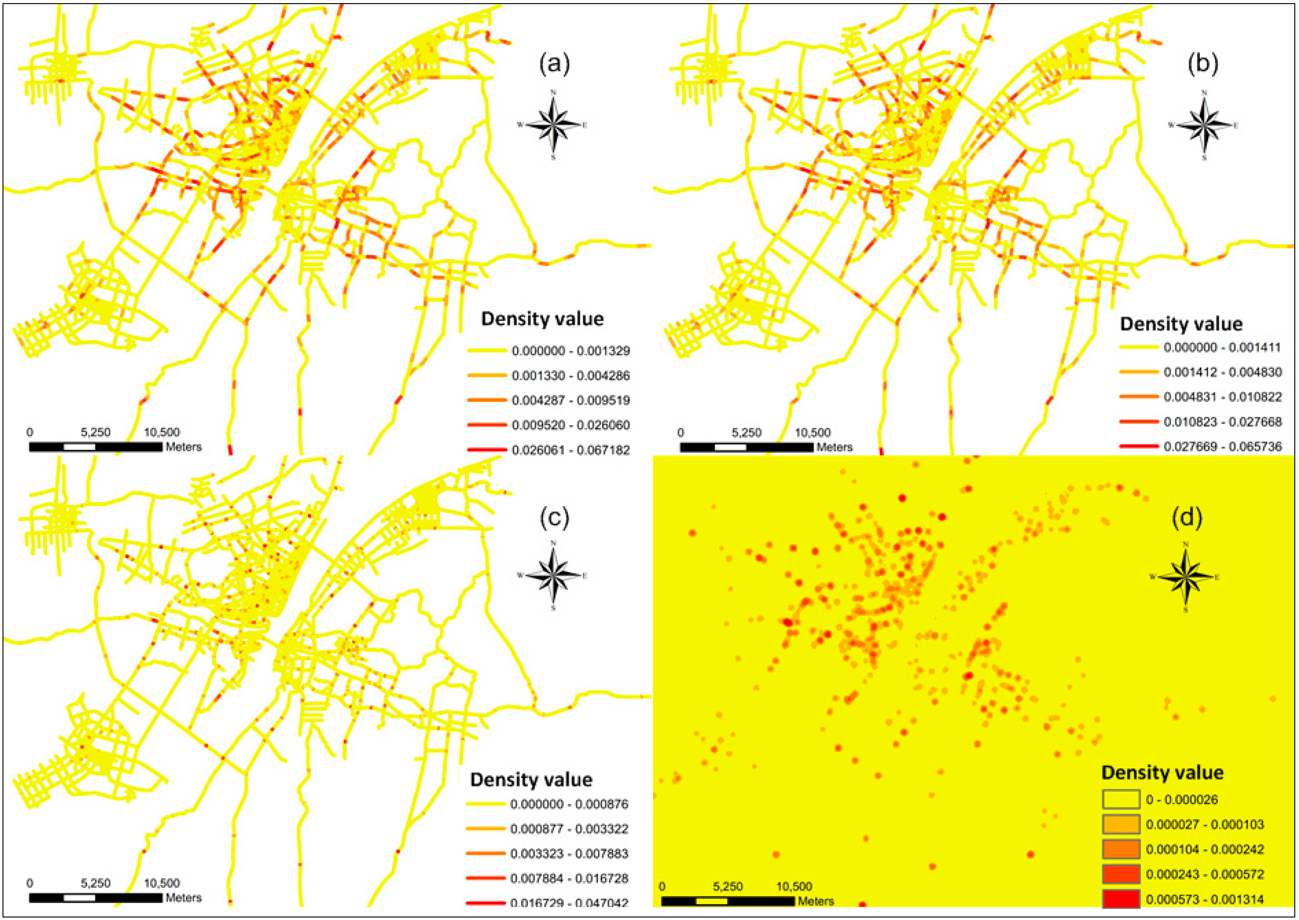
3.1. Results of the KDE and NKDE for Traffic Crash Events

| Experiments | 1 | 2 | 3 | 4 | |
|---|---|---|---|---|---|
| Parameters | Methods | NKDE | NKDE | NKDE | KDE |
| Length of lixel (m) | 10 | 10 | 40 | -- | |
| Search width (m) | 40 | 200 | 200 | 200 | |
| Kernel function | Gaussian | Gaussian | Gaussian | Gaussian | |
| Value | Count | 72,573 | 72,573 | 27,297 | -- |
| Min | 0 | 0 | 0 | 0 | |
| Max | 0.047234 | 0.067182 | 0.066892 | 0.001314 | |
| Sum | 20.544062 | 94.479292 | 32.121501 | 1.442635 | |
| Mean | 0.000283 | 0.001302 | 0.001177 | 0.000004 | |
| Standard Deviation | 0.001607 | 0.003499 | 0.00328 | 0.000027 | |

3.2. The GLINCS of NKDE
| Experiments | 5 | 6 | 7 | 8 | 9 | |
|---|---|---|---|---|---|---|
| Parameters | Input attribute | density value of experiments 2 | density value of experiments 3 | crash number | crash number | crash number |
| Lixel length | 10m | 40m | 10m | 40m | -- | |
| Simulation times | 99 | 99 | 99 | 99 | 99 | |
| Simulation type | Conditional Permutation | Conditional Permutation | Conditional Permutation | Conditional Permutation | Conditional Permutation | |
| p-value | 0.01 | 1126 | 431 | 0 | 0 | 14 |
| 0.05 | 1825 | 693 | 0 | 0 | 34 | |
| 0.1 | 2360 | 885 | 0 | 0 | 49 | |
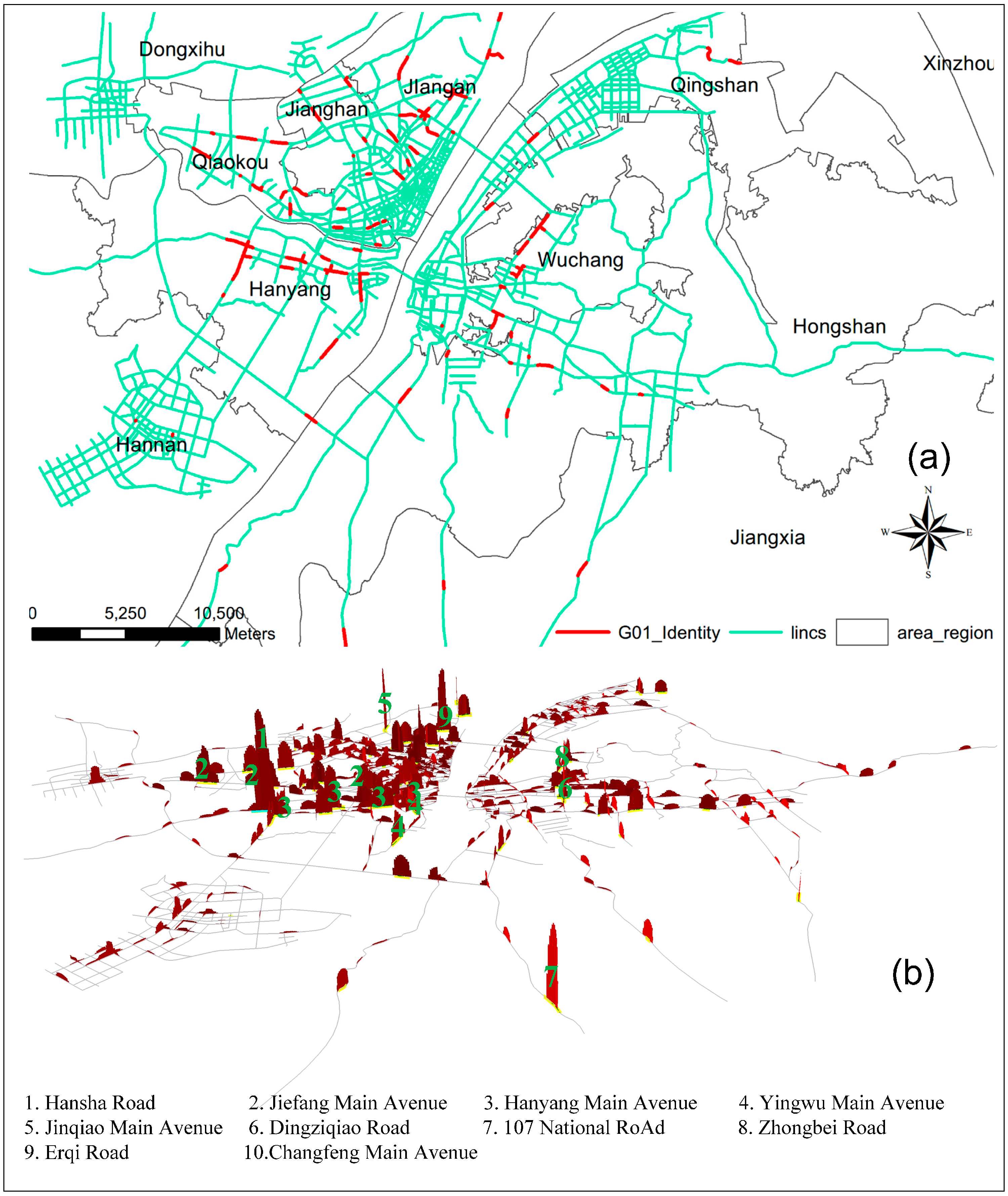
3.3. The Detection of Riskier Road Segments

| Order | Road Name | G* | Density Value (mean) | Z (mean) | Lixels (number) | District |
|---|---|---|---|---|---|---|
| 1 | Hansha Road | 0.0248 | 0.0409 | 10.6455 | 22 | Hanyang |
| 2 | Jiefang Main Avenue | 0.0217 | 0.0126 | 3.0175 | 63 | Qiaokou |
| 3 | Hanyang Main Avenue | 0.0192 | 0.0135 | 2.9929 | 56 | Jianghan |
| 4 | Yingwu Main Avenue | 0.0181 | 0.0126 | 3.3375 | 48 | Hanyang |
| 5 | Jinqiao Main Avenue | 0.0171 | 0.0248 | 7.0348 | 23 | Jiangan |
| 6 | Dingziqiao Road | 0.0131 | 0.0288 | 7.1706 | 17 | Hongshan |
| 7 | 107 National Road | 0.0149 | 0.0230 | 6.6381 | 21 | Jiangxia |
| 8 | Zhongbei Road | 0.0130 | 0.0110 | 2.6667 | 42 | Wuchang |
| 9 | Erqi Road | 0.0097 | 0.0228 | 4.6053 | 19 | Jiangan |
| 10 | Changfeng Main Avenue | 0.0117 | 0.0137 | 3.3258 | 31 | Qiaokou |
| 11 | Jianshe Main Avenue | 0.0110 | 0.0110 | 2.5378 | 37 | Qiaokou |
| 12 | Longyang Main Avenue | 0.0109 | 0.0089 | 2.6000 | 36 | Hanyang |
| 13 | Nianyihao Road | 0.0086 | 0.0102 | 2.4267 | 30 | Qingshan |
| 14 | Handti Street | 0.0085 | 0.0133 | 3.4000 | 22 | Jiangan |
| 15 | Xiongchu Main Avenue | 0.0076 | 0.0103 | 2.2714 | 28 | Hongshan |
| 16 | Zhongshan Main Avenue | 0.0060 | 0.0129 | 2.3000 | 22 | Qiaokou |
| 17 | Sanyanqiao Road | 0.0060 | 0.0182 | 3.8071 | 14 | Jiangan |
| 18 | Yongqing Road | 0.0058 | 0.0137 | 2.7889 | 18 | Jiangan |
| 19 | Jiangda Road | 0.0063 | 0.0127 | 2.9000 | 19 | Jiangan |
| 20 | Donghu Road | 0.0049 | 0.0096 | 1.9476 | 21 | Wuchang |
4. Summary and Conclusions
Acknowledgments
Author Contributions
Conflicts of Interest
References
- Wu, T.; Zhao, H.; Ou, X. Vehicle Ownership Analysis Based on GDP per Capita in China: 1963–2050. Sustainability 2014, 6, 4877–4899. [Google Scholar] [CrossRef]
- Evans, L. Traffic Safety; Science Serving Society: Bloomfield Hills, MI, USA, 2004. [Google Scholar]
- Zhang, H.Y. Analyzing Traffic Accident Situation with Bayesian Network. Ph.D. Thesis, Jilin University, Changchun, Jilin, China, June 2013. [Google Scholar]
- Zhang, G.; Yau, K.K.W.; Zhang, X. Analyzing fault and severity in pedestrian-motor vehicle accidents in China. Accid. Anal. Prev. 2014, 73, 141–150. [Google Scholar] [CrossRef] [PubMed]
- Chen, D. Research and Application on Evaluation Methods of Wuhan Public Transportation System. Master’s Thesis, Wuhan University of Technology, Wuhan, Hubei, China, June 2010. [Google Scholar]
- Flak, M.A. Reducing accident impacts under congestion. In Traffic Congestion and Traffic Safety in the 21st Century: Challenges, Innovations, and Opportunities; American Society of Civil Engineers: New York, NY, USA, 1997. [Google Scholar]
- Prasannakumar, V.; Vijith, H.; Charutha, R.; Geetha, N. Spatio-temporal clustering of road accidents: GIS based analysis and assessment. Procedia-Soc. Behav. Sci. 2011, 21, 317–325. [Google Scholar] [CrossRef]
- Maher, M.J.; Mountain, L.J. The identification of accident blackspots: A comparison of current methods. Accid. Anal. Prev. 1988, 20, 143–151. [Google Scholar] [CrossRef] [PubMed]
- Schuurman, N.; Cinnamon, J.; Crooks, V.A.; Hameed, S.M. Pedestrian injury and the built environment: An environmental scan of hotspots. BMC Public Health 2009, 9, Article 233. [Google Scholar] [CrossRef]
- Moons, E.; Brijs, T.; Wets, G. Improving Moran’s Index to Identify Hot Spots in Traffic Safety. In Geocomputation and Urban Planning; Murgante, B., Borruso, G., Lapucci, A., Eds.; Springer: Berlin, Germany, 2009; pp. 117–132. [Google Scholar]
- Joly, M.-F.; Foggin, P.M.; Pless, I.B. Geographical and socio-ecological variations of traffic accidents among children. Soc. Sci. Med. 1991, 33, 765–769. [Google Scholar] [CrossRef] [PubMed]
- Holz-Rau, C.; Scheiner, J. Geographical Patterns in Road Safety: Literature Review and a Case Study from Germany. EJTIR 2013, 13, 99–122. [Google Scholar]
- Li, L.; Zhu, L.; Sui, D.Z. A GIS-based Bayesian approach for analyzing spatial-temporal patterns of intra-city motor vehicle crashes. J. Transp. Geogr. 2007, 15, 274–285. [Google Scholar] [CrossRef]
- Anderson, T.K. Kernel density estimation and K-means clustering to profile road accident hotspots. Accid. Anal. Prev. 2009, 41, 359–364. [Google Scholar] [CrossRef] [PubMed]
- Eckley, D.C.; Curtin, K.M. Evaluating the spatiotemporal clustering of traffic incidents. Comput. Environ. Urban Syst. 2013, 37, 70–81. [Google Scholar] [CrossRef]
- Dai, D. Identifying clusters and risk factors of injuries in pedestrian-vehicle crashes in a GIS environment. J. Transp. Geogr. 2012, 24, 206–214. [Google Scholar] [CrossRef]
- Levine, N.; Kim, K.E.; Nitz, L.H. Spatial analysis of Honolulu motor vehicle crashes: I. Spatial patterns. Accid. Anal. Prev. 1995, 27, 663–674. [Google Scholar] [CrossRef] [PubMed]
- Elvik, R. Evaluations of road accident blackspot treatment: A case of the iron law of evaluation studies? Accid. Anal. Prev. 1997, 29, 191–199. [Google Scholar] [CrossRef] [PubMed]
- Flahaut, B.; Mouchart, M.; Martin, E.S.; Thomas, I. The local spatial autocorrelation and the kernel method for identifying black zones: A comparative approach. Accid. Anal. Prev. 2003, 35, 991–1004. [Google Scholar] [CrossRef] [PubMed]
- Chini, F.; Farchi, S.; Ciaramella, I.; Antoniozzi, T.; Rossi, P.G.; Camilloni, L.; Valenti, M.; Borgia, P. Road traffic injuries in one local health unit in the Lazio region: Results of a surveillance system integrating police and health data. Int. J. Health Geogr. 2009, 8, 21. [Google Scholar] [CrossRef] [PubMed]
- Erdogan, S. Explorative spatial analysis of traffic accident statistics and road mortality among the provinces of Turkey. J. Saf. Res. 2009, 40, 341–351. [Google Scholar] [CrossRef]
- Loo, B.P.Y. The identification of hazardous road locations: A comparison of the blacksite and hot zone methodologies in Hong Kong. Int. J. Sustain. Transp. 2009, 3, 187–202. [Google Scholar] [CrossRef]
- Black, W.R.; Thomas, I. Accidents on Belgium's motorways: A network autocorrelation analysis. J. Transp. Geogr. 1998, 6, 23–31. [Google Scholar] [CrossRef]
- Getis, A. A history of the concept of spatial autocorrelation: A geographer’s perspective. Geogr. Anal. 2008, 40, 297–309. [Google Scholar] [CrossRef]
- Yamada, I.; Thill, J.C. Local indicators of network-constrained clusters in spatial point patterns. Geogr. Anal. 2007, 39, 268–292. [Google Scholar] [CrossRef]
- Okabe, A.; Yamada, I. The K-function method on a network and its computational implementation. Geogr. Anal. 2001, 33, 271–290. [Google Scholar] [CrossRef]
- Chaikaew, N.; Tripathi, N.K.; Souris, M. Exploring spatial patterns and hotspots of diarrhea in Chiang Mai, Thailand. Int. J. Health Geogr. 2009, 8, 36. [Google Scholar] [CrossRef] [PubMed]
- Carlos, H.A.; Shi, X.; Sargent, J.; Tanski, S.; Berke, E.M. Density estimation and adaptive bandwidths: A primer for public health practitioners. Int. J. Health Geogr. 2010, 9, 39. [Google Scholar] [CrossRef] [PubMed]
- Pulugurtha, S.S.; Krishnakumar, V.K.; Nambisan, S.S. New methods to identify and rank high pedestrian crash zones: An illustration. Accid. Anal. Prev. 2007, 39, 800–811. [Google Scholar] [CrossRef] [PubMed]
- Anderson, T. Comparison of spatial methods for measuring road accident ‘hotspots’: A case study of London. J. Maps. 2007, 3, 55–63. [Google Scholar] [CrossRef]
- Chainey, S.; Tompson, L.; Uhligm, S. The utility of hotspot mapping for predicting spatial patterns of crime. Secur. J. 2008, 21, 4–28. [Google Scholar] [CrossRef]
- Yu, H.; Liu, P.; Chen, J.; Wang, H. Comparative analysis of the spatial analysis methods for hotspot identification. Accid. Anal. Prev. 2014, 66, 80–88. [Google Scholar] [CrossRef] [PubMed]
- Yamada, I.; Thill, J.C. Comparison of planar and network K-functions in traffic accident analysis. J. Transp. Geogr. 2004, 12, 149–158. [Google Scholar] [CrossRef]
- Loo, B.P.Y.; Yao, S. The identification of traffic crash hot zones under the link-attribute and event-based approaches in a network-constrained environment. Comput. Environ. Urban Syst. 2013, 41, 249–261. [Google Scholar] [CrossRef]
- Mohaymany, A.S.; Shahri, M.; Mirbagheri, B. GIS-based method for detecting high-crash-risk road segments using network kernel density estimation. Geo-spat. Inf. Sci. 2013, 16, 113–119. [Google Scholar] [CrossRef]
- Young, J.; Park, P.Y. Hotzone identification with GIS-based post-network screening analysis. J. Transp. Geogr. 2014, 34, 106–120. [Google Scholar] [CrossRef]
- Okabe, A.; Satoh, T.; Sugihara, K. A kernel density estimation method for networks, its computational method and a GIS-based tool. Int. J. Geogr. Inf. Sci. 2009, 23, 7–32. [Google Scholar] [CrossRef]
- Erdogan, S.; Yilmaz, I.; Baybura, T.; Gullu, M. Geographical information systems aided traffic accident analysis system case study: City of Afyonkarahisar. Accid. Anal. Prev. 2008, 40, 174–181. [Google Scholar] [CrossRef] [PubMed]
- Okabe, A.; Yomono, H.; Kitamura, M. Statistical analysis of the distribution of points on a network. Geogr. Anal. 1995, 27, 152–175. [Google Scholar] [CrossRef]
- Okabe, A.; Okunuki, K. A computational method for estimating the demand of retail stores on a street network and its implementation in GIS. Trans. GIS 2001, 5, 209–220. [Google Scholar] [CrossRef]
- Okabe, A.; Okunuki, K.I.; Shiodem, S. The SANET toolbox: New methods for network spatial analysis. Trans. GIS 2006, 10, 535–550. [Google Scholar] [CrossRef]
- Xie, Z.; Yan, J. Kernel density estimation of traffic accidents in a network space. Comput. Environ. Urban Syst. 2008, 32, 396–406. [Google Scholar] [CrossRef]
- Sugihara, K.; Okabe, A.; Satoh, T. Computational method for the point cluster analysis on networks. GeoInformatica 2011, 15, 167–189. [Google Scholar] [CrossRef]
- Steenberghen, T.; Aerts, K.; Thomas, I. Spatial clustering of events on a network. J. Transp. Geogr. 2010, 18, 411–418. [Google Scholar] [CrossRef]
- Li, Q.; Zhang, T.; Wang, H.; Zeng, Z. Dynamic accessibility mapping using floating car data: A network-constrained density estimation approach. J. Transp. Geogr. 2011, 19, 379–393. [Google Scholar] [CrossRef]
- Shiode, S.; Shiode, N. Network-based space-time search-window technique for hotspot detection of street-level crime incidents. Int. J. Geogr. Inf. Sci. 2013, 27, 866–882. [Google Scholar] [CrossRef]
- Xie, Z.; Yan, J. Detecting traffic accident clusters with network kernel density estimation and local spatial statistics: An integrated approach. J. Transp. Geogr. 2013, 31, 64–71. [Google Scholar] [CrossRef]
- Bíl, M.; Andrášik, R.; Janoška, Z. Identification of hazardous road locations of traffic accidents by means of kernel density estimation and cluster significance evaluation. Accid. Anal. Prev. 2013, 55, 265–273. [Google Scholar] [CrossRef] [PubMed]
- Plug, C.; Xia, J.C.; Caulfield, C. Spatial and temporal visualization techniques for crash analysis. Accid. Anal. Prev. 2011, 43, 1937–1946. [Google Scholar] [CrossRef] [PubMed]
- Nakaya, T.; Yano, K. Visualising Crime Clusters in a Space-time Cube: An Exploratory Data-analysis Approach Using Space-time Kernel Density Estimation and Scan Statistics. Trans. GIS 2010, 14, 223–239. [Google Scholar] [CrossRef]
- O’Sullivan, D.; Unwin, D.J. Geographic Information Analysis; John Wiley & Sons: Hoboken, NJ, USA, 2003. [Google Scholar]
- Getis, A.; Ord, J.K. The analysis of spatial association by use of distance statistics. Geogr. Anal. 1992, 24, 189–206. [Google Scholar] [CrossRef]
- Ord, J.K.; Getis, A. Local spatial autocorrelation statistics: Distributional issues and an application. Geogr. Anal. 1995, 27, 286–306. [Google Scholar] [CrossRef]
- Peeters, A.; Zude, M.; Käthner, J.; Kanber, R.; Hetzroni, A.; Gebbers, R.; Ben-Gal, A. Getis–Ord’s hot-and cold-spot statistics as a basis for multivariate spatial clustering of orchard tree data. Comput. Electron. Agric. 2015, 111, 140–150. [Google Scholar] [CrossRef]
- Yamada, I.; Thill, J.C. Local indicators of network-constrained clusters in spatial patterns represented by a link attribute. Ann. Assoc. Am. Geogr. 2010, 100, 269–285. [Google Scholar] [CrossRef]
- Porta, S.; Latora, V.; Wang, F.; Strano, E.; Cardillo, A.; Scellato, S.; Iacoviello, V.; Messora, R. Street centrality and densities of retail and services in Bologna, Italy. Environ. Plan. B Plan. Des. 2009, 36, 450–465. [Google Scholar]
- Jones, A.P.; Haynes, R.; Kennedy, V.; Harvey, I.M.; Jewell, T.; Lea, D. Geographical variations in mortality and morbidity from road traffic accidents in England and Wales. Health Place 2008, 14, 519–535. [Google Scholar] [CrossRef] [PubMed]
- Wier, M.; Weintraub, J.; Humphreys, E.H.; Seto, E.; Bhatia, R. An area-level model of vehicle-pedestrian injury collisions with implications for land use and transportation planning. Accid. Anal. Prev. 2009, 41, 137–145. [Google Scholar] [CrossRef] [PubMed]
© 2015 by the authors; licensee MDPI, Basel, Switzerland. This article is an open access article distributed under the terms and conditions of the Creative Commons Attribution license (http://creativecommons.org/licenses/by/4.0/).
Share and Cite
Nie, K.; Wang, Z.; Du, Q.; Ren, F.; Tian, Q. A Network-Constrained Integrated Method for Detecting Spatial Cluster and Risk Location of Traffic Crash: A Case Study from Wuhan, China. Sustainability 2015, 7, 2662-2677. https://doi.org/10.3390/su7032662
Nie K, Wang Z, Du Q, Ren F, Tian Q. A Network-Constrained Integrated Method for Detecting Spatial Cluster and Risk Location of Traffic Crash: A Case Study from Wuhan, China. Sustainability. 2015; 7(3):2662-2677. https://doi.org/10.3390/su7032662
Chicago/Turabian StyleNie, Ke, Zhensheng Wang, Qingyun Du, Fu Ren, and Qin Tian. 2015. "A Network-Constrained Integrated Method for Detecting Spatial Cluster and Risk Location of Traffic Crash: A Case Study from Wuhan, China" Sustainability 7, no. 3: 2662-2677. https://doi.org/10.3390/su7032662