1. Introduction
GNSS relative positioning has been widely applied in many fields, such as structural health monitoring [
1], crustal motion monitoring [
2], mine deformation monitoring [
3], and attitude determination [
4]. For short to medium baselines, common errors with respect to different receivers can be regarded as being well canceled, such as satellite orbit and clock errors, ionospheric and tropospheric delay errors. However, multipath errors and some other random noises are still remained. This can be clearly seen in the carrier phase measurement residual series, as shown in the following figures. Systematic patterns can be easily seen even by the naked eye, which violates the assumption of purely random noises. These systematic patterns are deemed the effect of multipath errors. According to its mechanism, the magnitude of multipath error can be as high as a quarter of the signal wavelength [
5,
6,
7]. In general, the effects of multipath errors cannot be ignored in the above-mentioned high precision applications. Work should be conducted to model and mitigate the influences of the multipath errors.
Due to the complex physical and geometrical characteristics of the surrounding environment reflecting GNSS signals, constructing a theoretical model of multipath errors is rather difficult. However, extracting an empirical model from the data is still possible. Multipath error is the main constituent of the measurement residual, however contaminated by noise. The feasibility of modeling multipath errors using the noisy measurement residuals lies in the fact that the multipath is somewhat systematic, while the noise is purely random. Empirical multipath error modeling has been widely studied in recent years. Multipath error models of either carrier phase/code pseudorange measurements or site coordinates can be constructed, with names “observation-domain” or “positioning-domain”, respectively [
8,
9]. Multipath error modeling can be done in time domain, namely viewing multipath error as a function of time, or phase of the period, using techniques such as wavelet thresholding denoising [
10,
11], multi-resolution analysis [
12,
13], Vondrak filtering [
14], empirical mode decomposition [
15,
16] and stochastic state estimation [
17]; it can also be done in space domain, namely viewing multipath error as a function of satellite elevation and azimuth angles, using techniques such as gridding [
18,
19], polynomial [
20] and harmonic models [
21]. After a multipath model has been constructed by processing a dataset, it can be used to mitigate the effects of the multipath errors in the same dataset, and also those in other datasets, e.g., data collected in the future. For the latter case, the mitigation can be done in real time; and when time domain modeling is adopted, it is often called sidereal filtering [
22]. In sidereal filtering, it is vital to determine the repeat time of the multipath errors [
23,
24,
25,
26].
In this contribution, an alternative method is proposed for GNSS carrier phase measurement multipath error modeling in time domain. In this method, multipath error modeling is regarded as a (multipath) signal reconstruction problem. The systematic characteristic of the multipath errors implies certain extent of smoothness, which is exploited using Tikhonov regularization [
27]. The first and the second order derivative regularizations are both considered. Efficient numerical algorithms, namely Thomas algorithm or Cholesky rank-one update, are devised to solve the problem by exploiting the specific structure of the normal equations [
28]. Regularization coefficients, namely Lagrange multipliers, are optimized through bootstrap technique [
29].
The rest of the paper is organized as follows.
Section 2 is devoted to methodology development, including calculating the carrier phase measurement residuals, modeling with first order derivative regularization, modeling with second order regularization and determining regularization coefficients using bootstrap. Experiment analysis is presented in
Section 3 and concluding remarks are given in
Section 4.
2. Methods
Carrier phase measurement residuals generation, modeling with the first and the second order derivative regularization and regularization coefficient optimization are developed in line in the following subsections.
2.1. Generating Carrier Phase Measurement Residuals
Double difference mode is chosen as an example; the same or similar methodology can be applied to other modes, e.g., single or zero difference. At epoch
k, the linearized measurement equation is as follows:
where
y denotes the observed minus computed carrier phase measurement vector;
B denotes the design matrix;
x denotes the constant baseline coordinates;
τ denotes the differenced clock error;
e denotes measurement error vector including multipath signal and other noises. Let the cofactor matrix corresponding to (1) be denoted as
Qk, and the estimated vector of
x at the immediately previous epoch be denoted as
, with cofactor matrix
. This estimated vector can be viewed as a pseudo measurement vector besides the real one as in (1). This, we have the following augmented measurement equation:
with cofactor
. The least-squares solution to is as follows:
The estimated vector of unknown parameters, , is assigned to , and the corresponding part of the cofactor matrix is assigned to , which are used as prior parameter vector and the corresponding cofactor at the next epoch. At the first epoch, the augmented measurement equation as in reduces to the real measurement Equation (1). After all data used to model multipath signals are processed recursively according to the above procedure, a final estimated vector of x is obtained, denoted as . Substitute this estimate, along with the epoch-by-epoch clock error estimates, into the measurement equation at each epoch, the residuals are obtained as an estimate of the errors ek. These residuals are exactly the “raw” data to be processed to modeling the multipath signals. The main idea lies in extracting the relatively smooth multipath signal from the noisy residuals. This is exactly a denoising problem, also called a signal reconstruction issue or filtering process.
Note that available RTK software can also be used to generate the carrier phase residuals.
2.2. Denoising with First-Order Derivative Regularization
The denoising/filtering/reconstruction problem is solved by exploiting the smoothness of the multipath signal. Tikhonov regularization will be applied for dealing with this kind of issue [
27]. For an arbitrary satellite, the corresponding residual series are denoted as {
ϕk}. The measurement equation for the problem is as follows:
where
m and
η denote multipath signal and noise, respectively. The target function for the first regularization problem is constructed as:
where
w denotes the weight depending on the satellite elevation; λ denotes the Lagrange multiplies, which is a hyperparameters to be optimized in
Section 2.4. The matrix form of (5) is as follows:
with an (
n − 1) ×
n Tikhonov matrix
expressed as follows:
The minimizer of (6) satisfies the following necessary condition,
Although analytical solution to the above equation exists, it should not be employed in practice. The dimension of problem as in (8) is often very high, namely tens of thousands. Directly solving so large equations would be rather time consuming. Fortunately, fast algorithm exists for our specific problem, mainly due to the special structure of
, and hence of
. To be more specific,
N is a symmetric tridiagonal matrix, as shown below:
Thus, the numerically efficient tridiagonal matrix algorithm can be used to solve (8). The tridiagonal matrix algorithm (TMA), also called the Thomas algorithm, is exactly a Gaussian elimination algorithm tailored to consider the tridiagonal structure [
28]. As
N is both diagonally dominant and positive definite, TMA has no stability problems. The algorithmic flow of TMA is as follows. First, a forward sweep is recursively evaluated:
Then the solution is obtained by back substitution.
This completes the development of the modeling with the first order derivative regularization. The number of floating-point operations (flops) involved in TMA, namely in performing (10)~(12), is 15n − 15. Considering that matrix inversion, which is the most involved part in least-squares, involves ≈2n3 flops, there is a significant, namely a two-order improvement, in computational efficiency with TMA.
2.3. Denoising with Second-Order Difference Regularization
Similar to (5), we have the following cost function for the modeling with the second order derivative regularization:
with its vector-matrix form
with an (
n − 2) ×
n Tikhonov matrix
expressed as follows:
According to the first order necessary condition for optimization, the solution is as follows:
Let
, then the matrix inversion in (16) can be rearranged as follows:
According to Shermann-Morrison formula, the above inversion can be evaluated recursively using the following Cholesky rank-one update.
Let
. Let the 3 × 3 submatrix of
Mk−1 starting from
kth row and
kth column be denoted as
Uk. Then we have:
which are used in the update of (18). The location of the submatrix
in
is the same as that of
Uk in
Mk−1. That means that in each iteration as in (18), only nine elements need to be updated. After the final update of (18), we have
. There are 2
n2 + 100
n − 200 flops involved in this rank-one update based method, namely in evaluating (16) and (18)–(20), in order. This is an order higher than the computational complexity of the TMA for the first-order difference regularization, however is still an order lower than that of the general method.
2.4. Determining Regularization Coefficients Using Bootstrap
As an empirical model, modeling errors are inevitable. The modeling errors are assessed using the bootstrap method [
29]. Regularization coefficient corresponding to the minimum modeling error is selected. Determine the candidate set of the regularization coefficients, e.g.,
.
For each coefficient, perform the modeling process described in
Section 2.2 or
Section 2.3. Define the following normalized residual (residual of the carrier phase measurement residuals:
It is easy to see that this residual series is homoscedastic. We randomly sample from the above normalized residual series with replacement to obtain series {
φk}. Add series {
φk/
wk} to
to obtain a resampled measurement vector
. Repeat this resampling process
B times (try
B = 50). For the
bth resampled measurement vector, 1 ≤
b ≤
B, perform the modeling described in
Section 2.2 or
Section 2.3, Let the corresponding estimate be denoted as
or
. The argument
λ/
μ is introduced intentionally to denote the dependence on the regularization coefficients. Let the following average be the final estimate for the corresponding regularization coefficients:
The subscript 0 denote the solution obtained in
Section 2.2 or
Section 2.3 using the raw measurement. The solution in (22), often called bootstrap estimate, is believed, in general, to be better than the one obtained using only the raw measurement. Define the following error statistics:
These error statistics denote the overall modeling errors with different modeling strategies (first or second derivative regularization) and different hyper parameters (
λ/
μ). Finally, the regularization coefficient is determined as follows:
Note again that the estimate with these coefficient as in (22) is exactly the final estimate, which is used to correct measurement at the same time of the next day.
3. Results
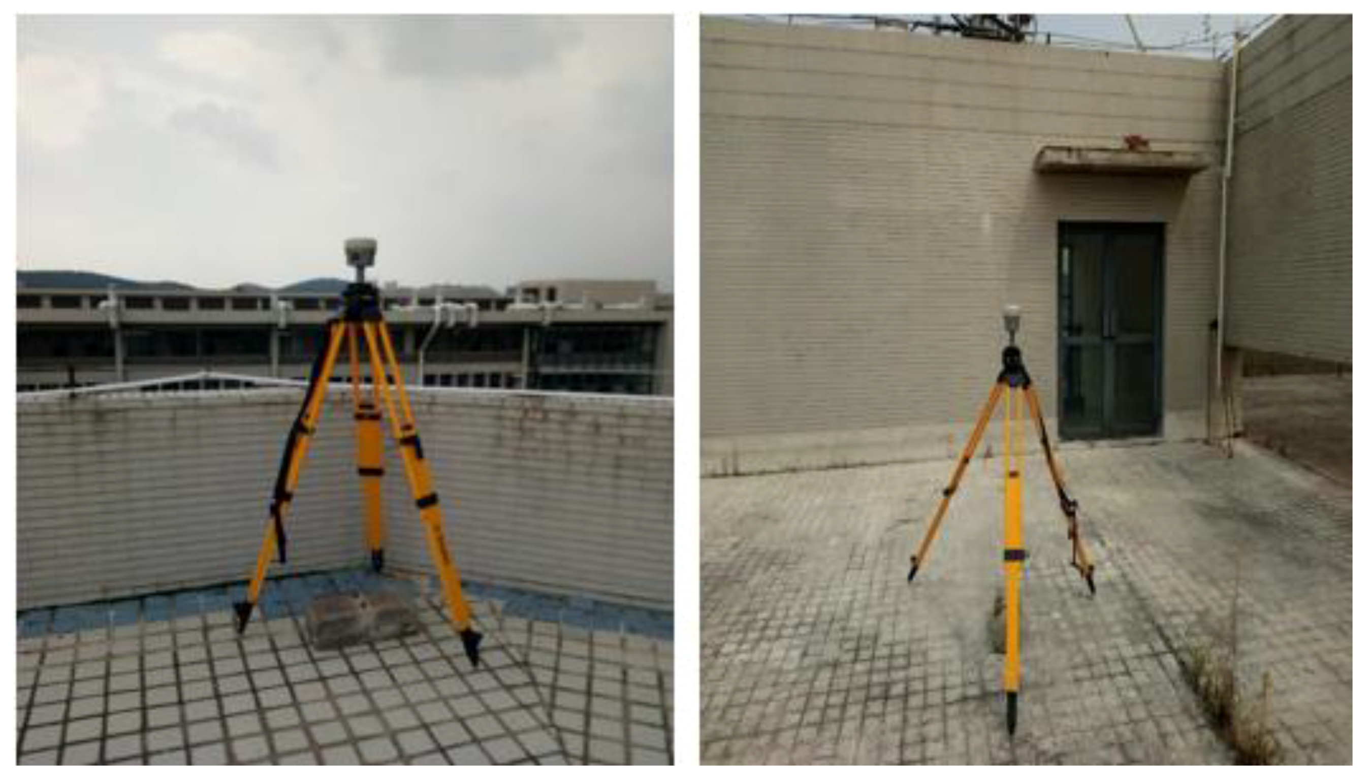
In order to verify the consistency between orbital period and multipath periods of Global Position System (GPS) satellites and the feasibility of the regularization method, we calculated the residuals and extracted the multipath model with respect to each satellite, and evaluated the baseline results. A short period and a long period dataset were collected to verity the performance of the proposed methods, respectively. The short dataset was collected on 29 September 2017 to 2 October 2017, from 10:00 AM to 11:30 AM, named Day 1–4. Another was collected from 8:30 AM to 11:40 AM on 5 October 2017 to 8 October 2017, named Day 5–8. The sample rate of both the datasets was set at 1 Hz and with 10° elevation mask angle at the roof of School of Environmental Science and Spatial Informatics, China University of Mining and Technology. One antenna is mounted on an empty corner with an unobstructed environment, as the base station. Another antenna is placed about 5 m away from the southeast direction of a white wall as the rover station. The two GNSS receivers are Trimble R10 units and the length of the baseline is about 62.210 m. The locations for two receivers are shown in
Figure 1. To ensure that the base station is not affected by multipath effects and the rover station has a significant multipath effect, we turned off the anti-multipath function of the rover station, while switching on the function of the base station. The processing using the proposed method is developed based on GNSS data processing software RTKLIB [
30]. First, GPS observations of the previous day were processed in the static mode; and then on the following days, the coordinates of the rover station at each epoch were estimated independently in the post-processing kinematic mode with integer ambiguities fixing, and with or without the aid of the multipath modeling [
31].
As mentioned in the introduction, one key of sidereal filtering is to estimate multipath repeat time accurately. There are three commonly used methods for estimating the repeat time: orbit repeat time method (ORTM) [
25], aspect repeat time adjustment (ARTA) [
24] and residual correlation method (RCM) [
8]. The different mechanisms and algorithms of the three can be found in [
26]. Without loss of generality, in this work, we adopt RCM.
According to the steps in [
31,
32], we calculated the L1 phase residuals of different GPS satellites.
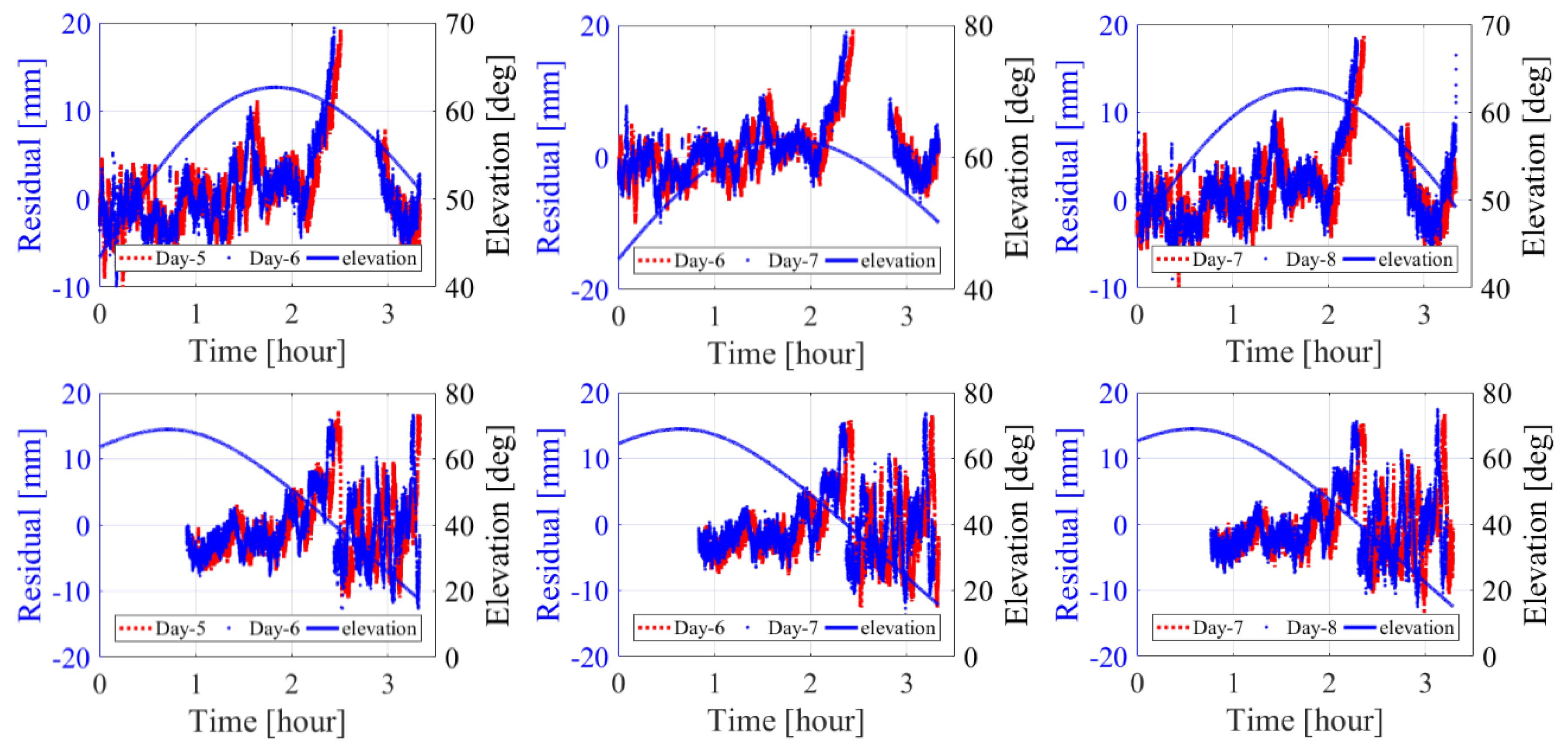
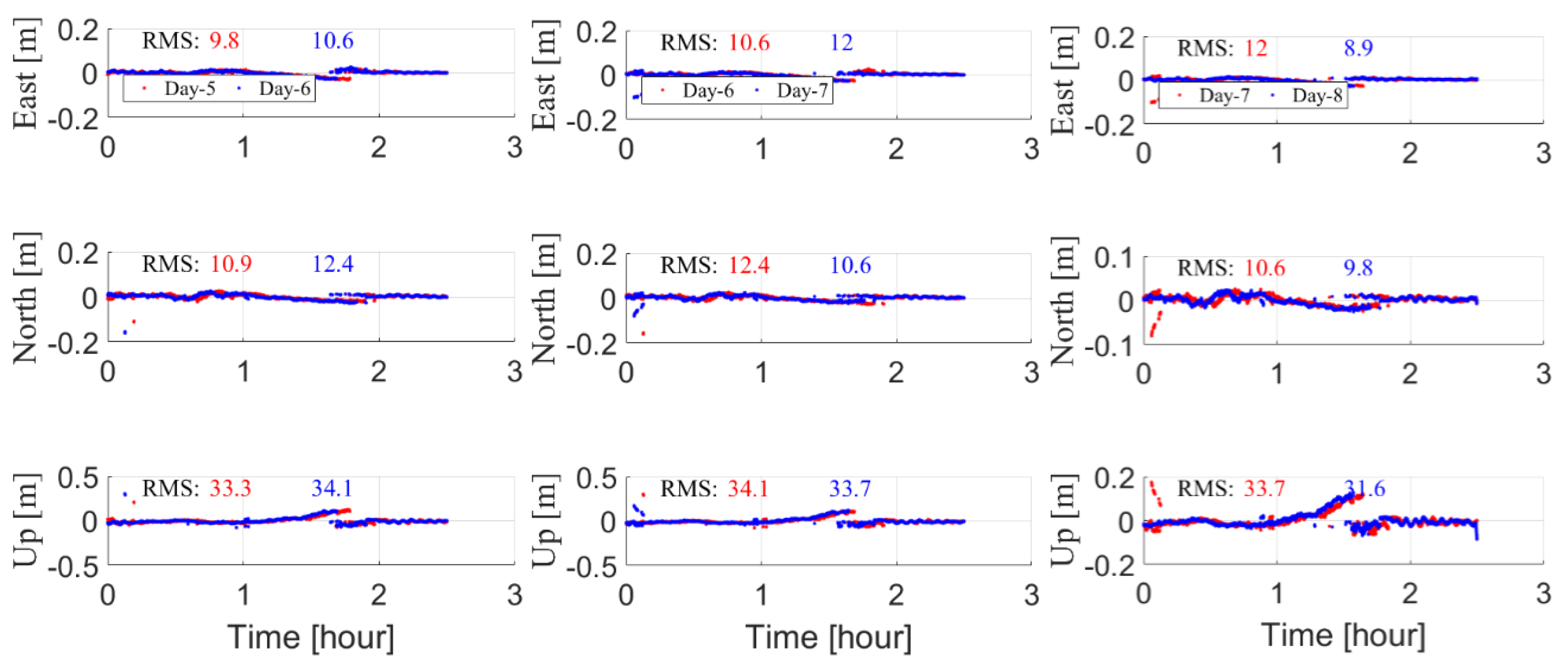
Figure 2 shows phase measurement residuals of G06 and G17 through Day 5–8 with static mode processing. Similarly, baseline coordinate residuals are shown in
Figure 3. For each plot of
Figure 2 and
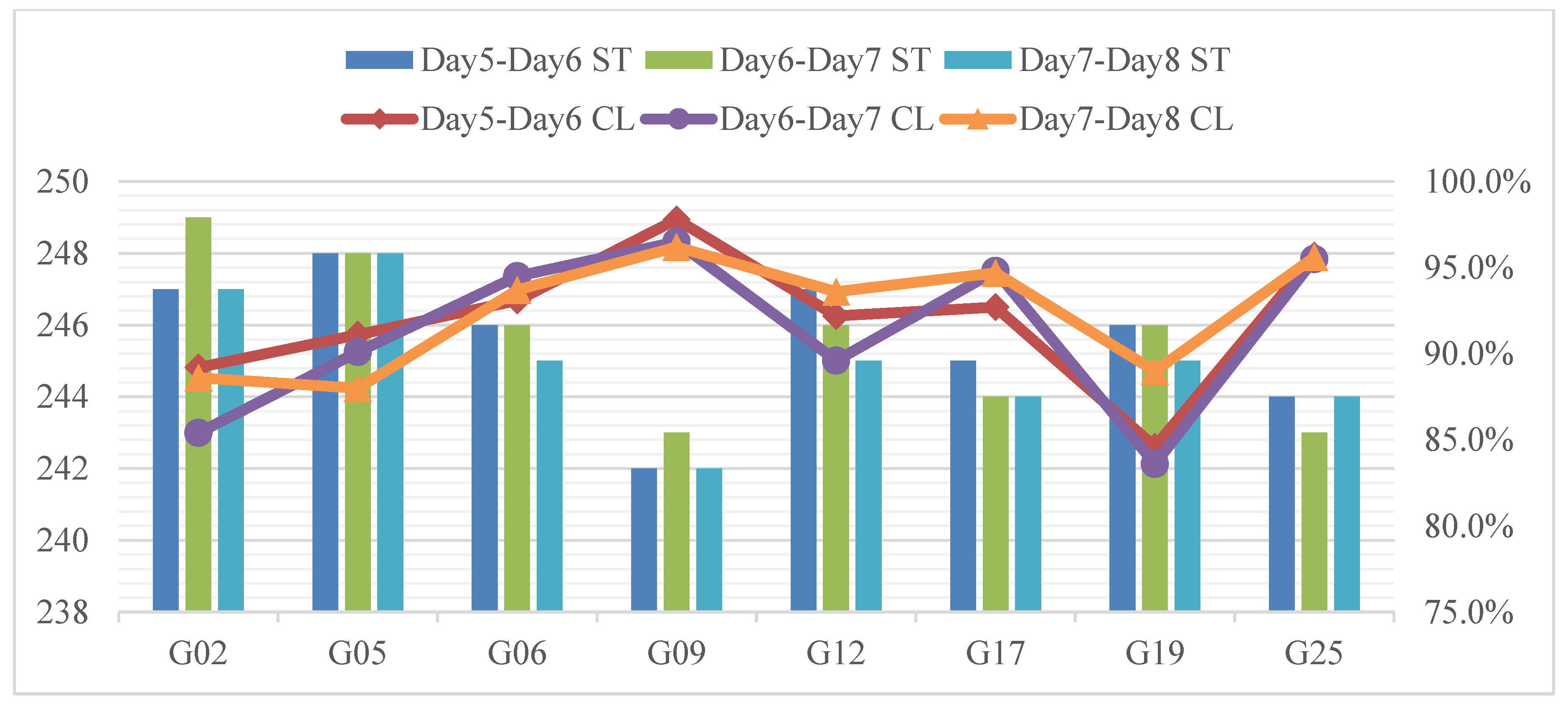
Figure 3, the results of two adjacent days are illustrated together to explicitly show the correlations between the two days. From the two figures, we can observe that there are strong correlations between the two adjacent periods, not only for phase measurement residuals, but also for baseline coordinate residuals. We calculated the multipath repeat time using RCM, namely finding the shift time making the correlation coefficient maximum. The multipath repeat time, transformed to time shift and the correlation coefficients between adjacent periods are given in
Figure 4. As we can see in
Figure 2,
Figure 3 and
Figure 4, the residuals in observation domain and coordinate domain almost repeated themselves every sidereal day in the three consecutive days. As the periodical variation of phase residuals, namely multipath error, results from the periodic motion of the corresponding satellite, the orbital repeat period is the same as the multipath cycle time when the environment around antennas is not changed. The mean residual time shift when correlation coefficient is maximum value is 245 s and the mean of correlation coefficient is up to 91.9% in spite of the existence of uncorrelated noises in consecutive days. This strongly implies the feasibility of the sidereal filtering methods, namely mitigating the multipath errors in one dataset based on the model developed using the dataset on the immediately previous sidereal day, according to the orbital repeat time.
The data of Day 1–3 and 5–7 were processed in static model with ambiguity fixing. The phase residuals and coordinate components were estimated epoch by epoch. Carrier phase measurement residuals corresponding to different satellites and the corresponding multipath errors extracted using different methods are shown in
Figure 5. The standard deviations (STD) of the three series are also displayed. To get an intuitive expression concerning the performance of the proposed method relative to other existing methods, the wavelet soft-thresholding denoising method is chosen as an example to be compared in the data processing. The chosen wavelet basis function is sym6, the decomposition layer is 4, and the threshold is default provided by MATLAB. For brevity, only the results of one satellite on one day are shown for Day 5–7, the results on Day 1–3 are similar. The main observations from these figures are the following: first, the modeled multipath errors clearly capture the main pattern of the measurement residuals and second, the multipath errors are relatively smoother than the carrier phase measurement residuals. Considering that the multipath error is extracted from the carrier phase measurement residual, the first observation implies the fidelity of the former to the latter, and the second implies the denoising effect of the proposed method. Another observation, which can be quantitatively shown by the standard deviations, is that the performance of second-order regularization method is only slightly better than the first-order, and that both regularization methods provide slightly better smoothness than the wavelet soft-thresholding denoising method.
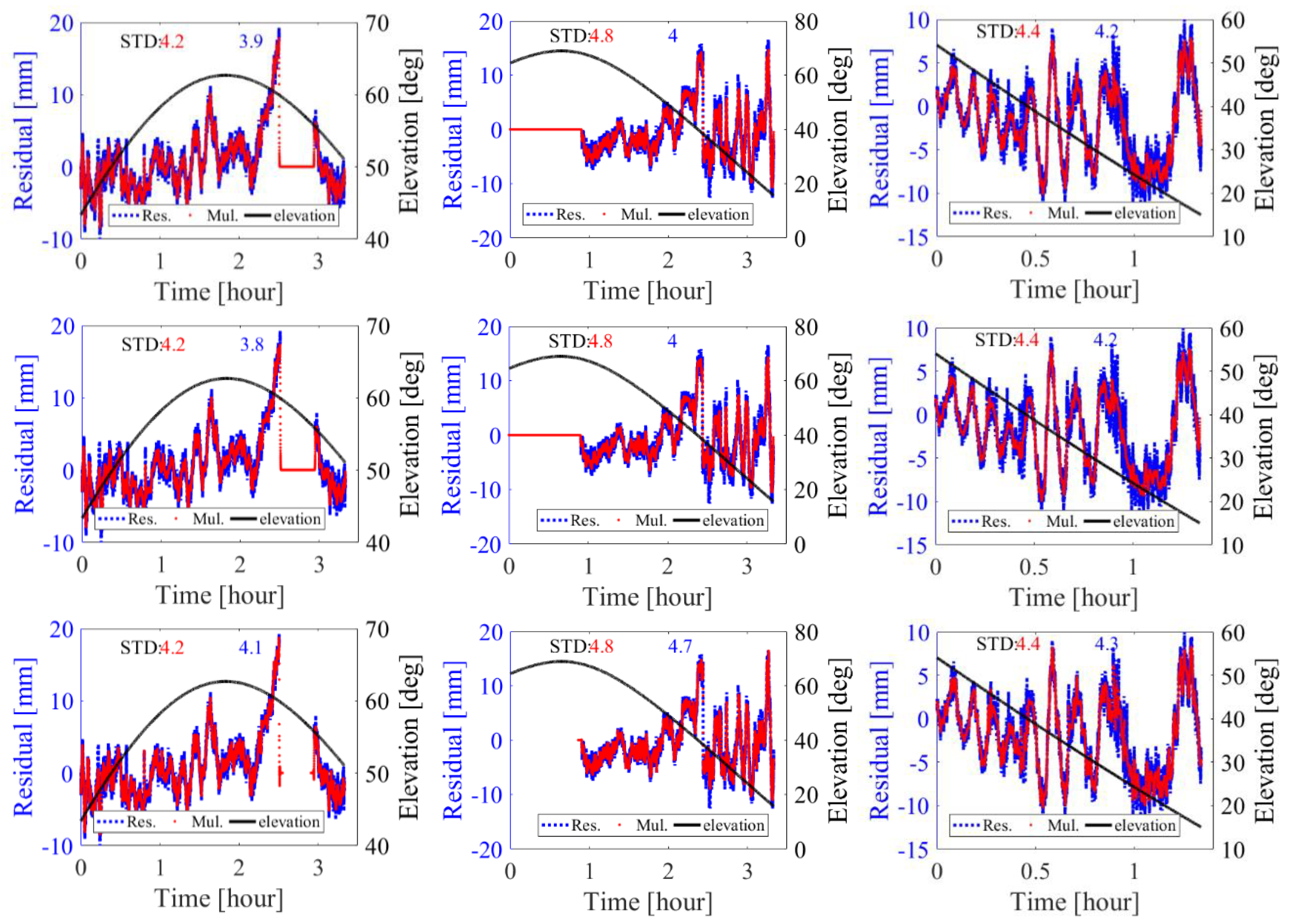
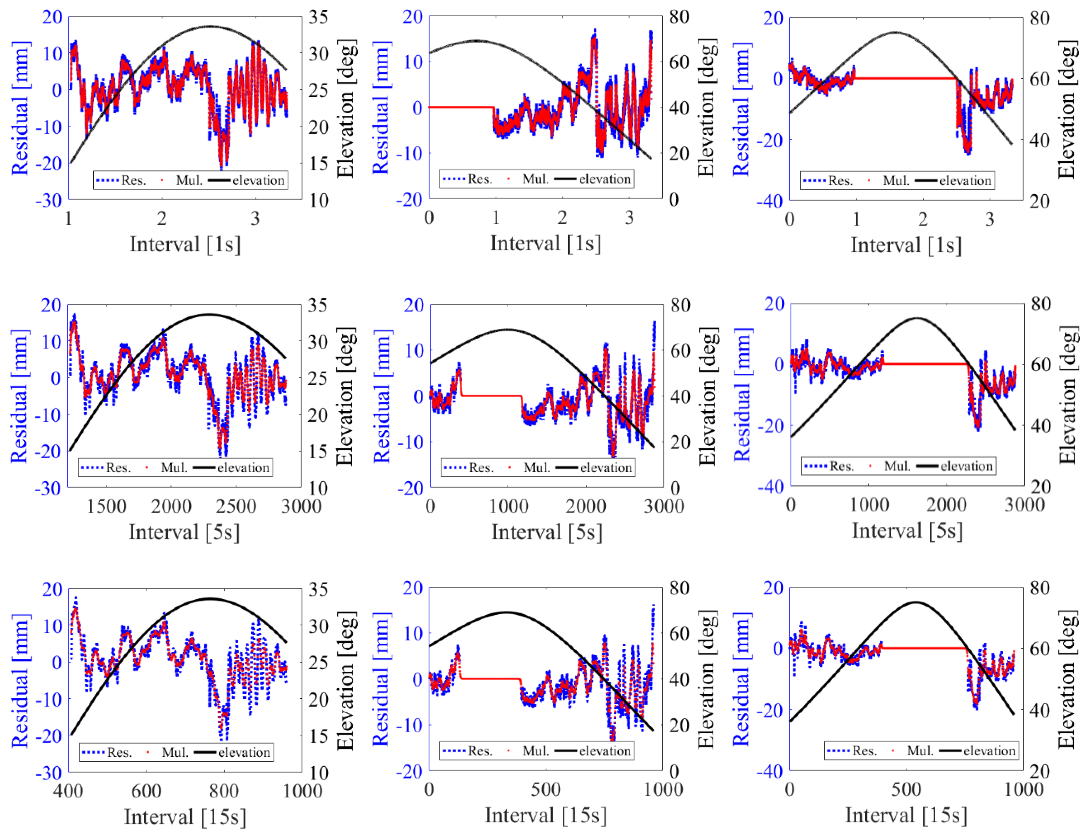
In order to test the performance of proposed method with different sample interval, we down-sampled the original data with 5 s and 15 s intervals.
Figure 6 shows the carrier phase measurement residuals and multipath errors extracted using the first order Tikhonov regularization method with 1 s, 5 s, and 15 s intervals. Two statements are made from this figure: First, with larger sampling intervals, the proposed method can still capture the pattern of the multipath errors; second, the smoothness of the constructed model clearly decreases as the sampling interval increases. The second statement can be easily explained, the down-sampled data themselves, from which the model is extracted, are not so smooth as the original one. The root-mean-squares of the raw residuals and those after being corrected with the extracted multipath error models are tabulated in
Table 1. From this table, it is clearly shown that the modeling accuracy is relatively low with sparser data. Besides the lower modeling accuracy, the applicability of the down-sampled-data modeling also decreased: interpolation is needed to correct higher-rate data using models from lower-rate data. This suggests that data with higher sampling rate should be used in modeling.
The sidereal filtering performance using the proposed method is checked in the following.
Figure 7 shows the phase residuals before and after multipath effects mitigation (sidereal filtering) with first-order, second-order Tikhonov regularization methods and wavelet soft-thresholding denoising, respectively. From
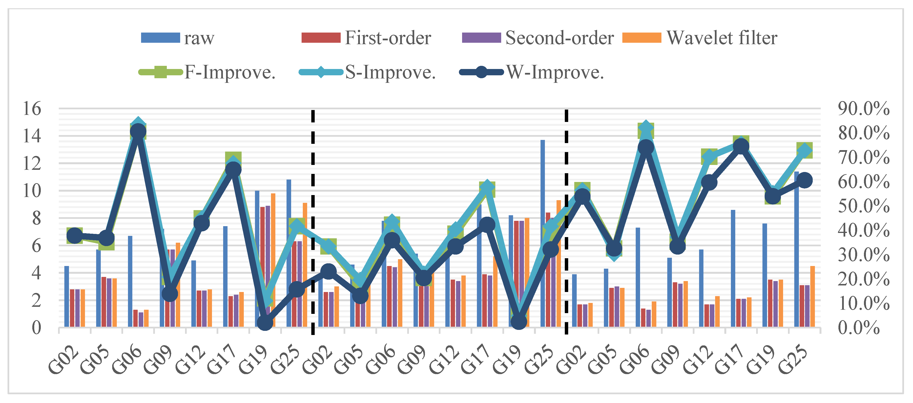
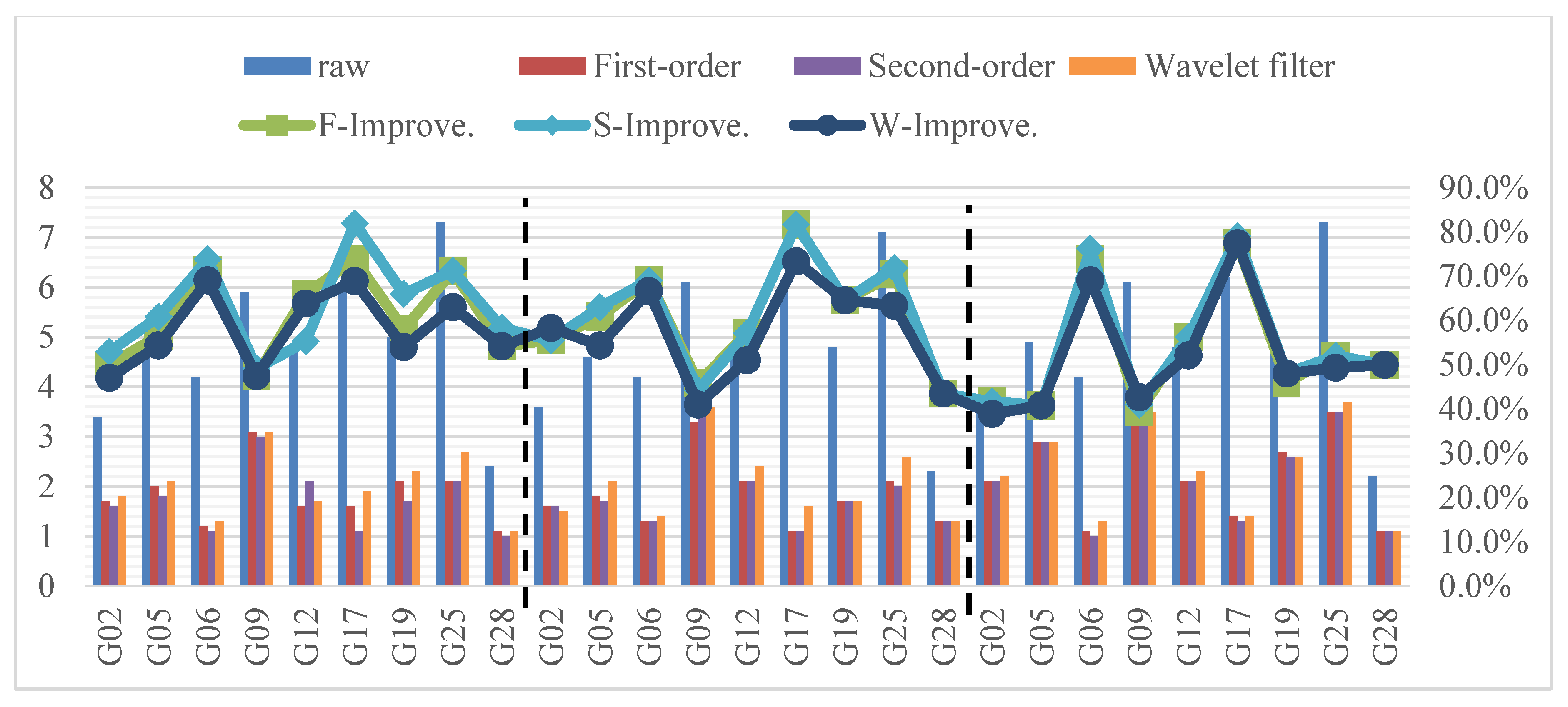
Figure 7, it can be easily seen that systematic patterns, which are significant in raw residuals, almost disappear in the residuals with multipath mitigated. This shows the efficacy of the three multipath modeling approaches. The RMS values of the residuals before and after sidereal filtering and the percentages of improvements on Day 2–4 and Day 6–8 are shown in
Figure 8 and
Figure 9, respectively. From
Figure 8 and
Figure 9, the average percentages of improvements across all visible satellites for first order regularization/second order regularization/wavelet soft-thresholding are 44.6%/45.3%/39.1% and 58.3%/59.5%/55.8% on Day 2–4 and Day 6–8, respectively. From
Figure 8 and
Figure 9, the following three can be observed: First, the measurement residuals decrease significantly after sidereal filtering with any of the three modeling approaches. This is a quantitative validation of the observation made from
Figure 7. Second, the proposed method, with either of the two regularizations, produces relatively smaller residuals than the wavelet soft-thresholding denoising method, though the difference can still be viewed as slight. Third, the performances of the first-order and the second-order regularization approaches are almost the same.
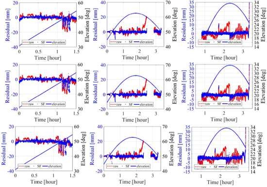
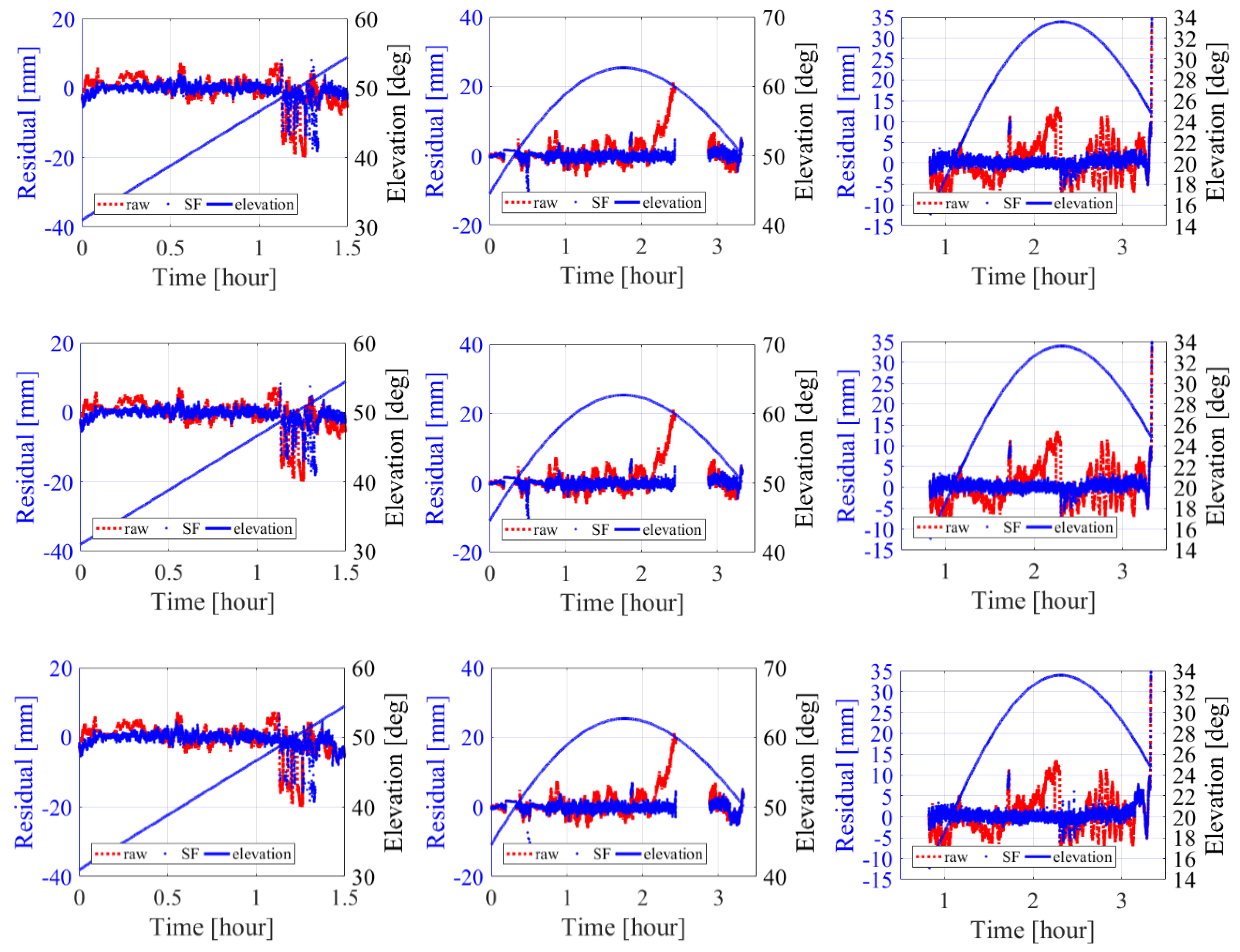
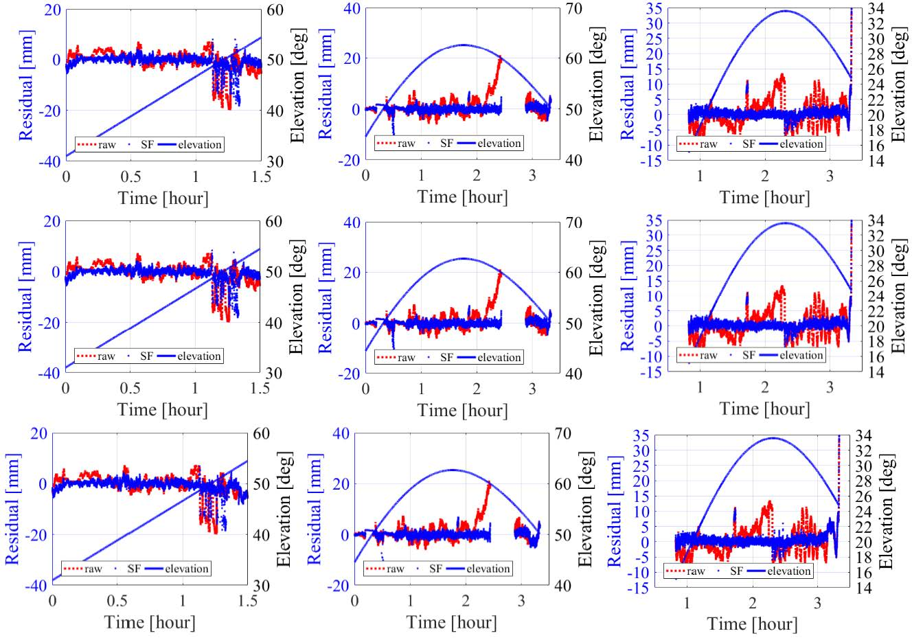
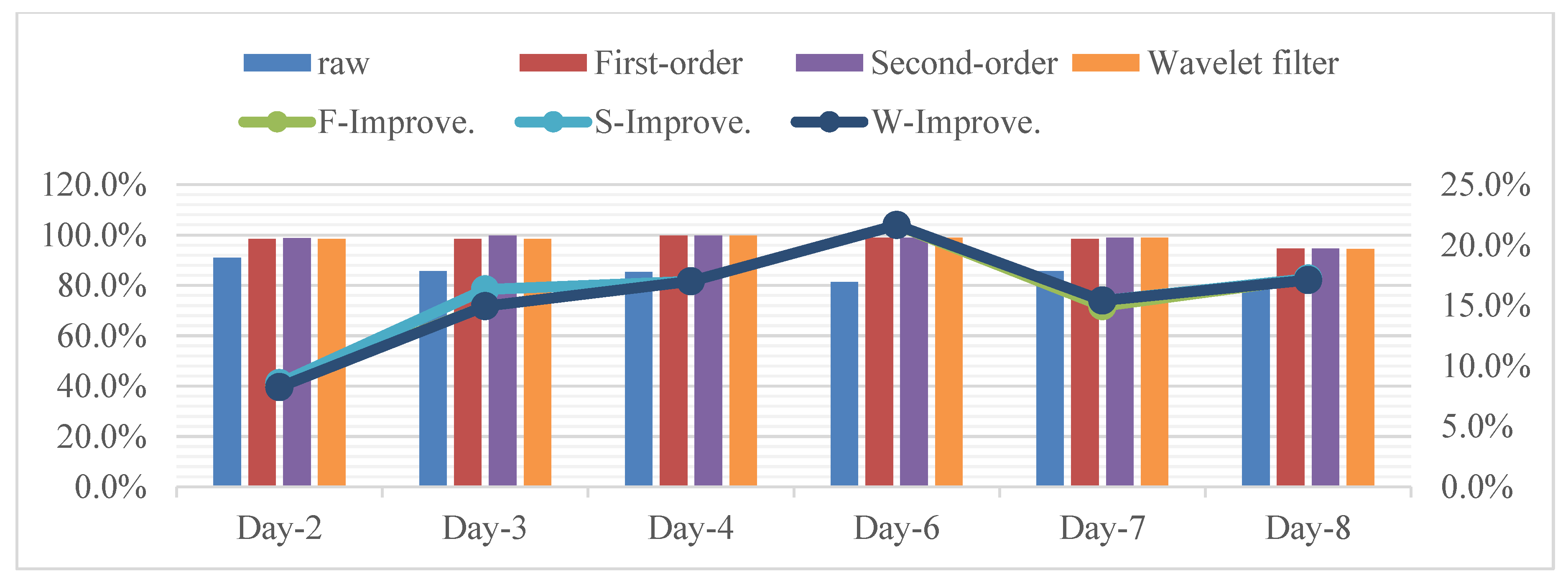
The direct consequence of the multipath error will decrease the rate of ambiguity fixing. The merit of the proposed method will be confirmed if the ambiguity fixing rate improves after multipath mitigation. We tested the data of Day 5–8. From
Figure 10,
Figure 11 and
Figure 12, it is clearly shown that the ambiguities were not fixed correctly during the first hour if the multipath errors are not mitigated. The ambiguity fixing rates before and after sidereal filtering mitigation of multipath errors are shown in
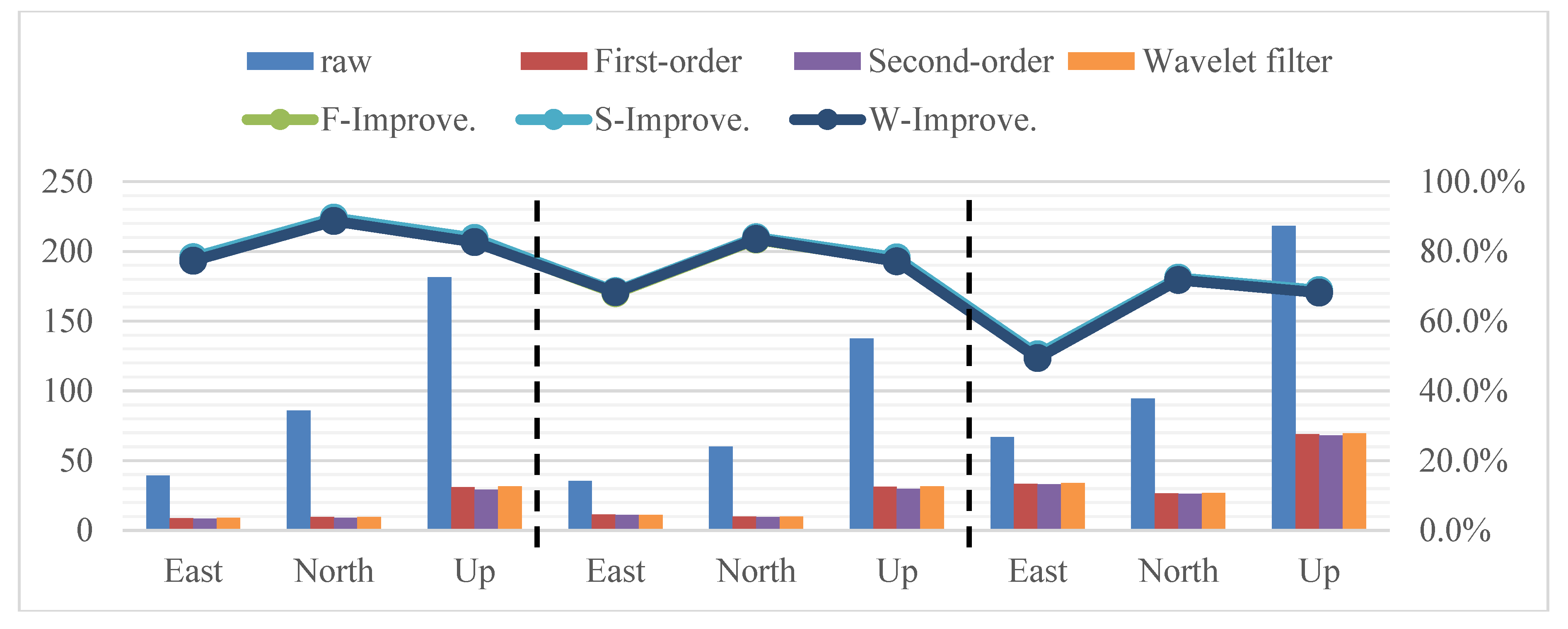
Figure 13. From these figures, we can find that after multipath mitigation, the percentages improvements in ambiguity fixing rates with first-order, second-order regularizations and wavelet filtering are 17.9%/18.1%/18.1% in average on Day 6–8. The RMSs of the coordinate residuals before and after sidereal filtering mitigation of multipath errors and the corresponding percentages of improvements are shown in
Figure 14. The average improvements along E/N/U directions after first-order, second-order regularizations and wavelet filtering are 65.2%/81.5%/76.2%, 65.8%/82.0%/77.0% and 65.0%/81.3%/76.0% in average on Day 6–8, respectively.
The significant improvement of the positioning accuracy shown in
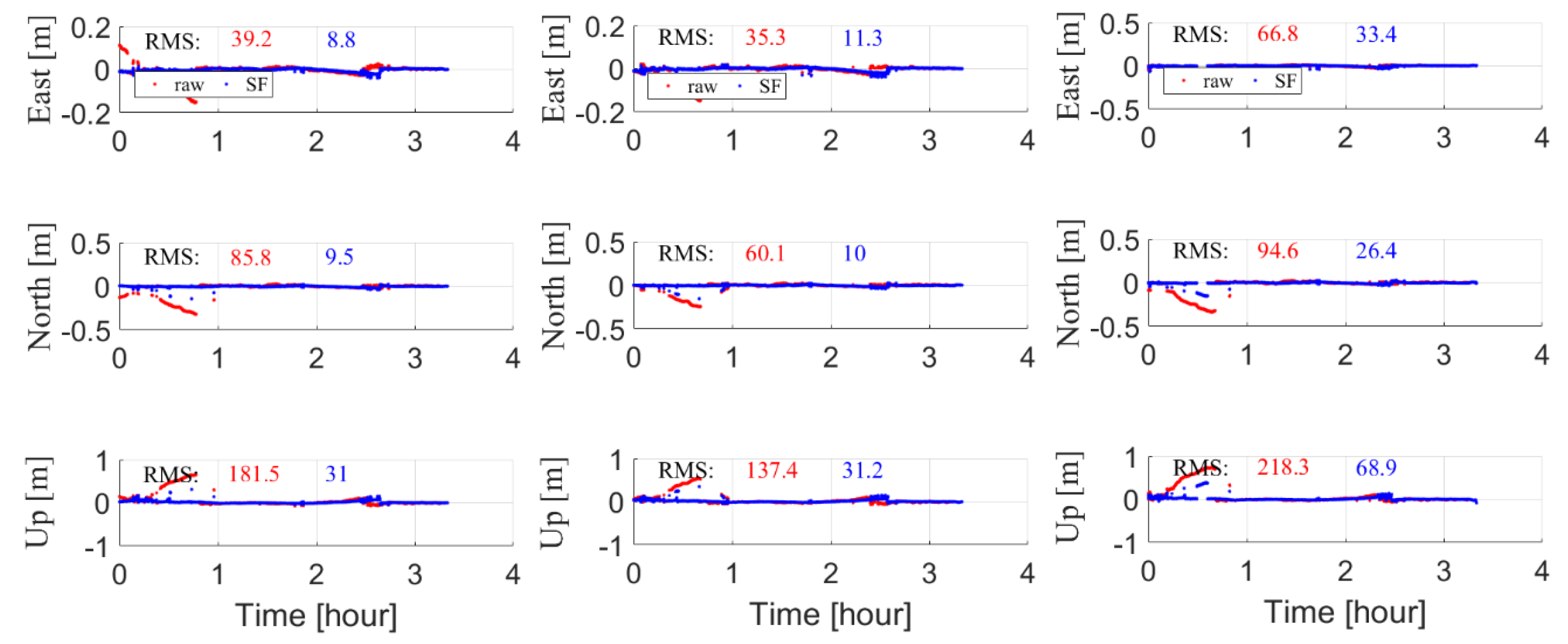
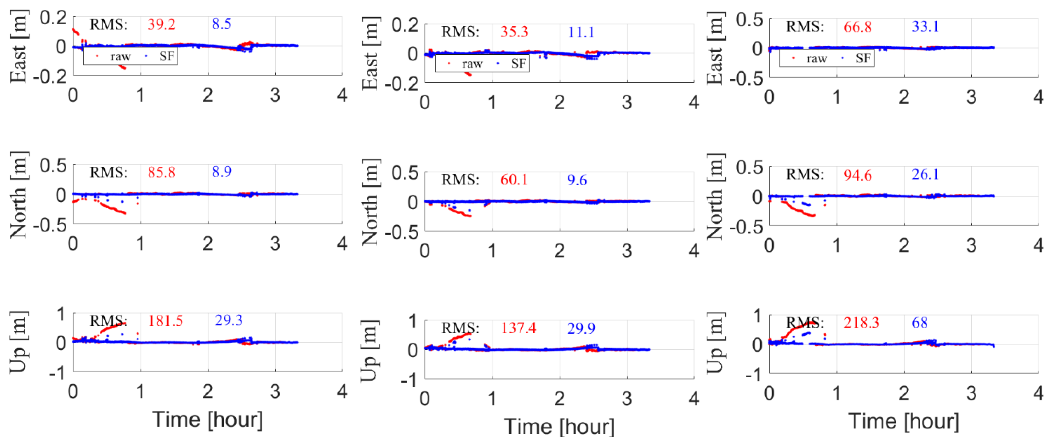
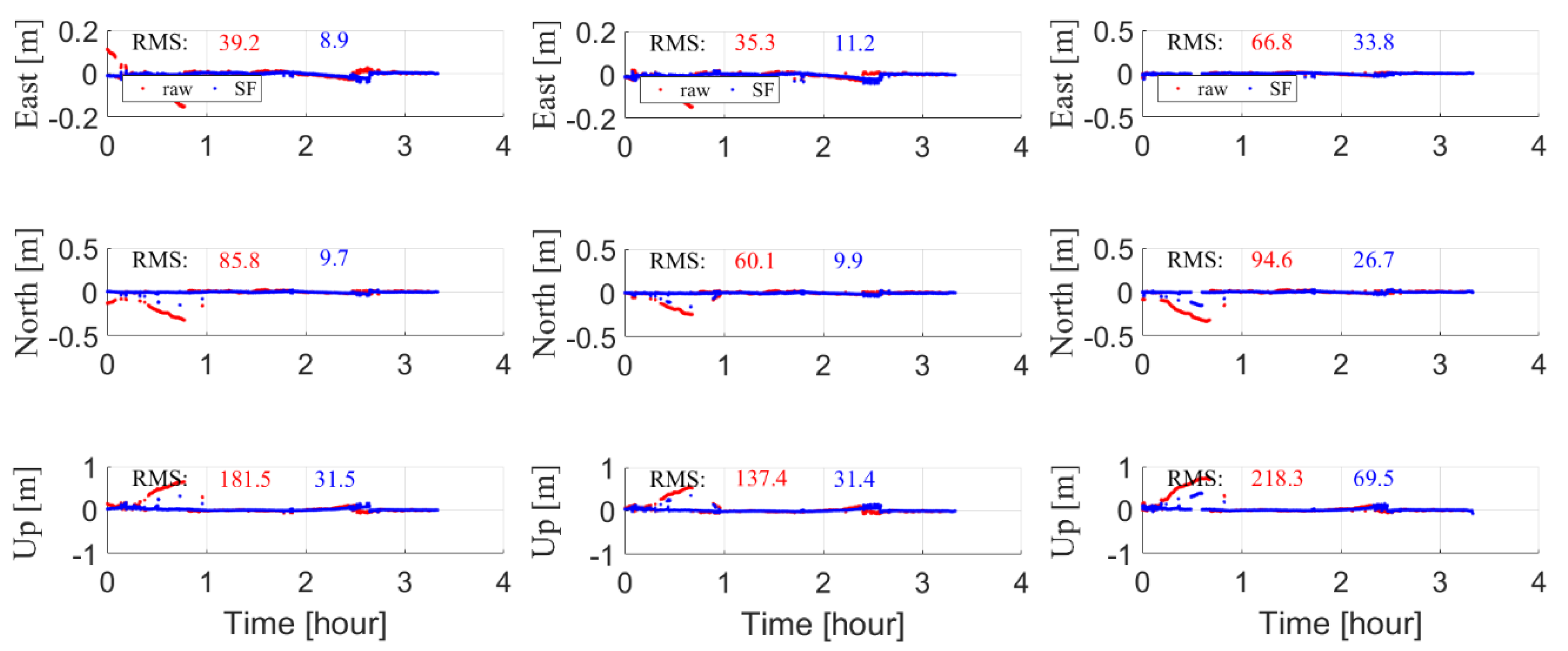
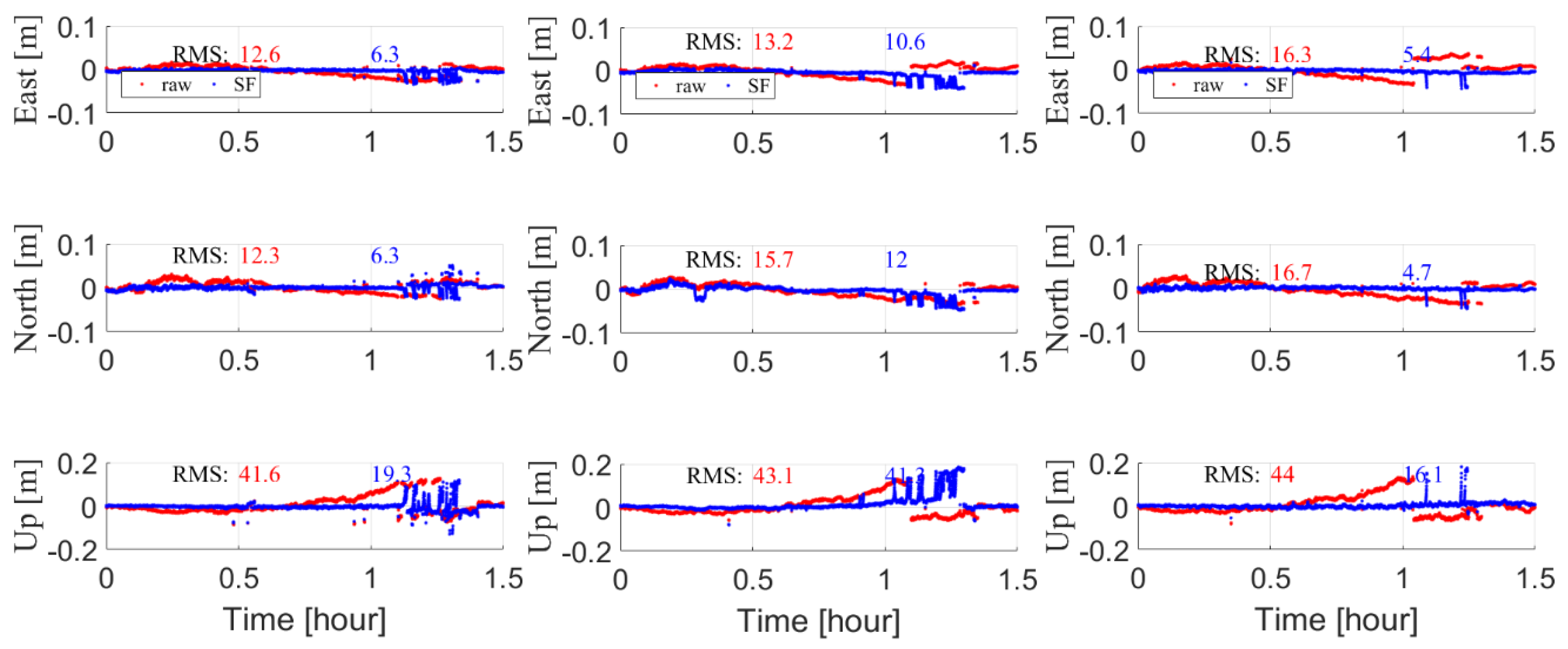
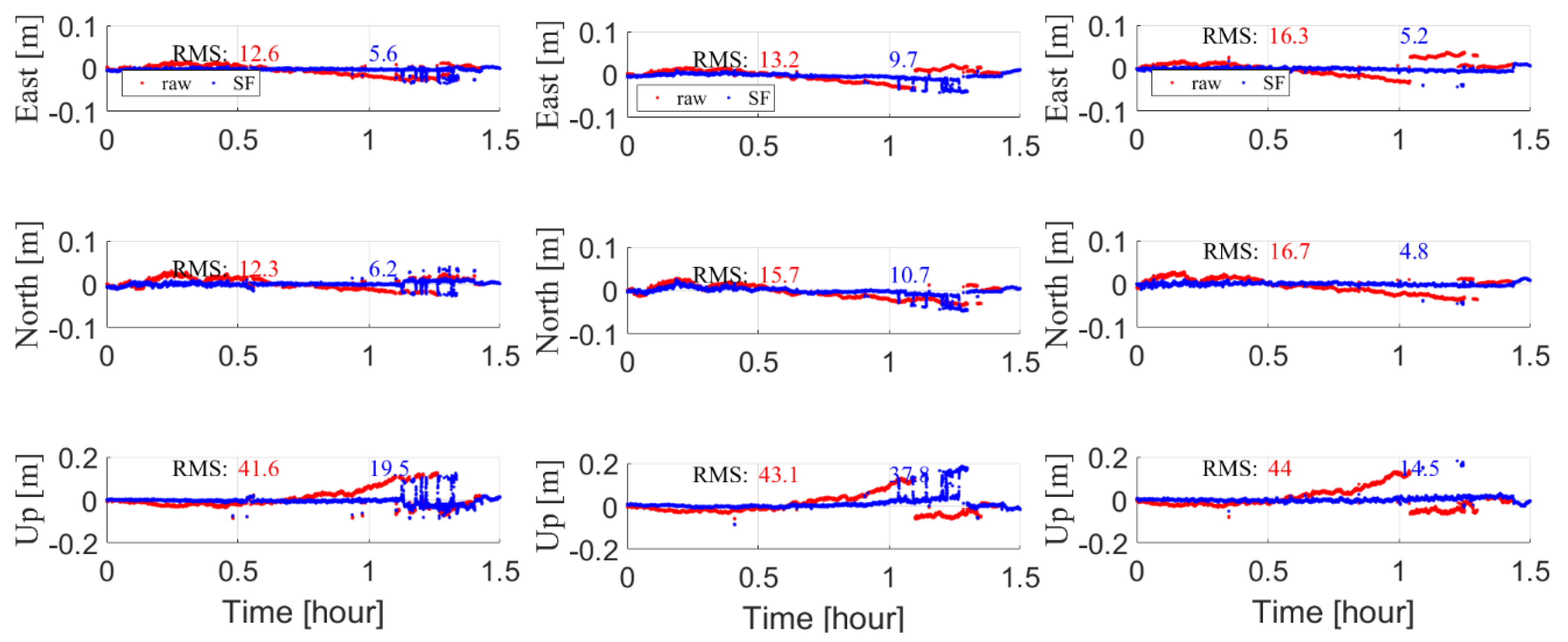
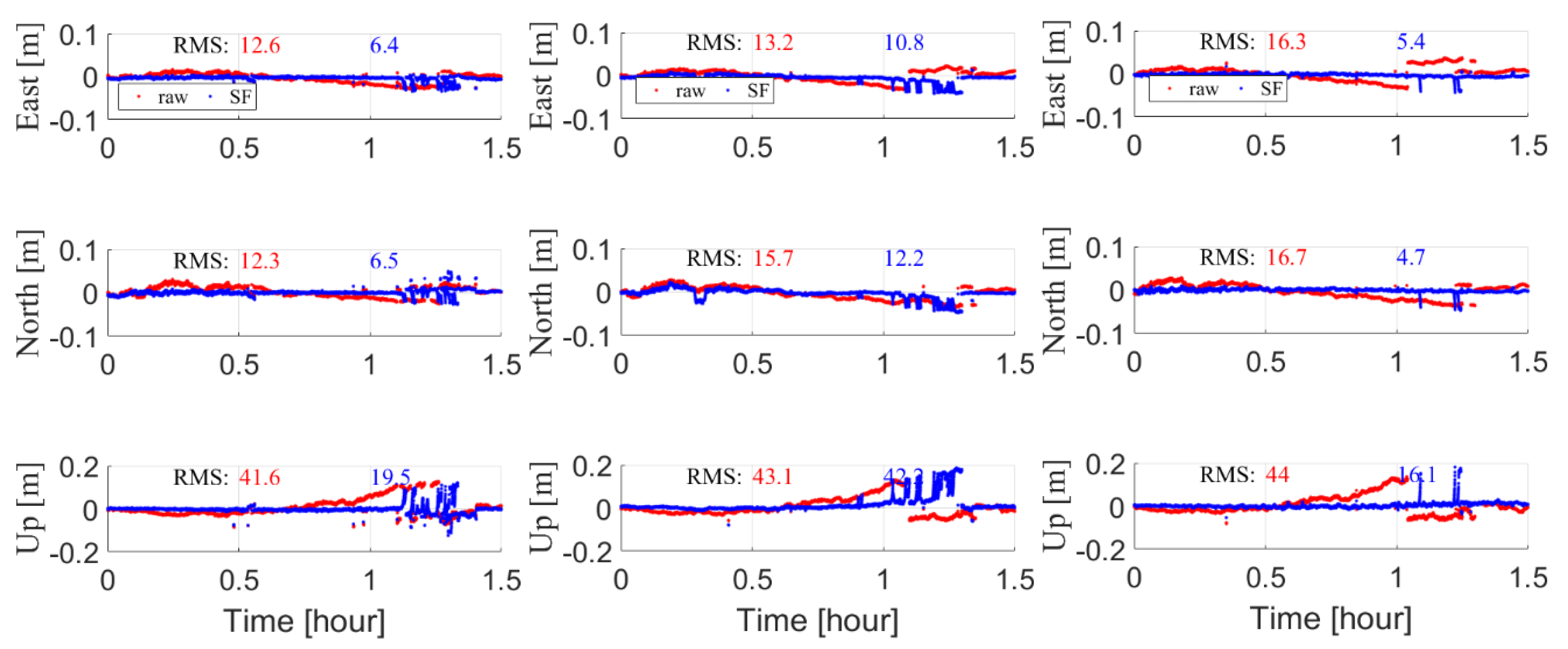
Figure 14 should largely due to the increased ambiguity fixing rates. It is naturally interesting to know whether or how the accuracy is improved on the basis of similar ambiguity fixing. The data of Day 2–4 are selected. The results, namely the baseline coordinates residuals, are shown in
Figure 15,
Figure 16 and
Figure 17. From these figures, the merits of sidereal filtering mitigation of multipath errors are conformed in terms of positioning accuracy, for either of the three modeling approaches. The main observations from these figures are the following: first, after the multipath mitigation, it can be easily seen that systematic patterns, which are significant in raw-data baseline coordinate residuals in East, North and Up directions, almost disappear in the residuals with multipath mitigated. The ambiguity fixing rate is again increased after multipath mitigation, as shown in
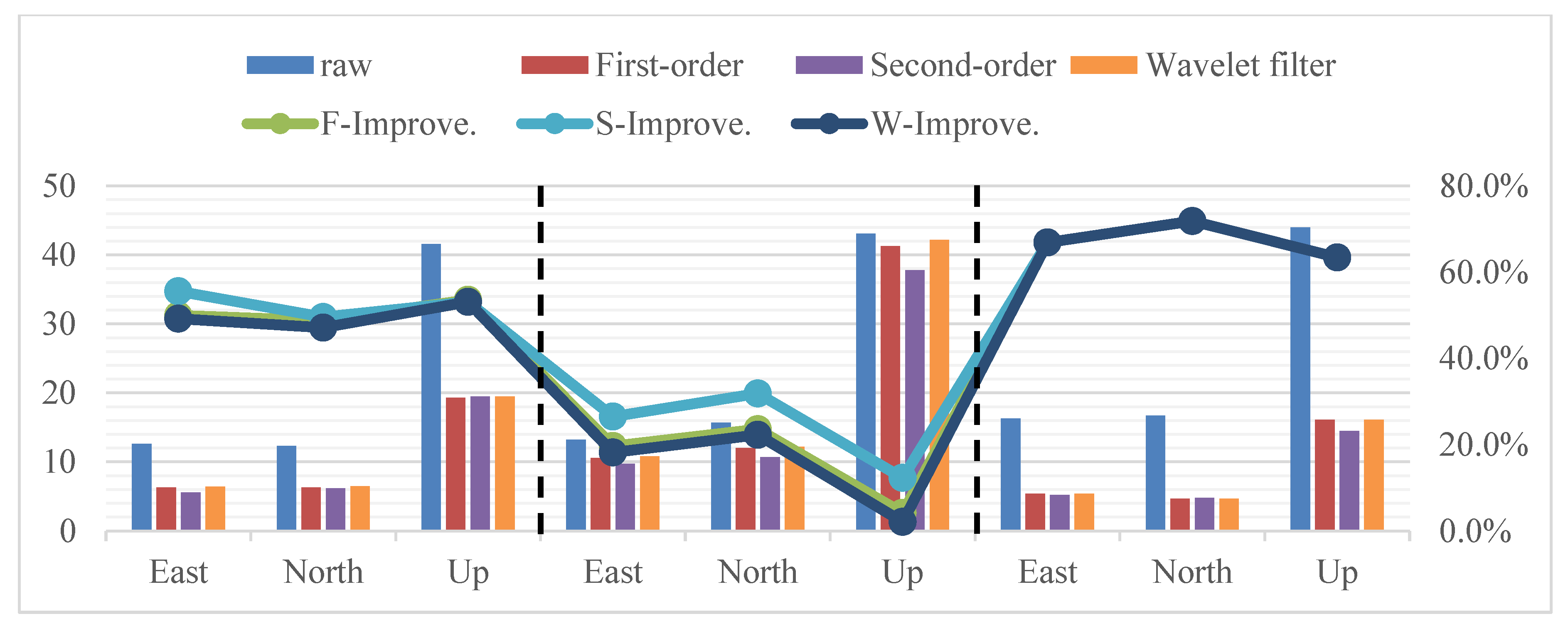
Figure 13. During 11:00–11:30 AM on Day 2–4, there are several epochs with extremely poor positioning results in all figures. These degraded performances should be due to wrong ambiguity fixings. The RMS of baseline coordinate residuals before and after sidereal filtering mitigation of multipath errors and the corresponding percentages of improvements for this dataset are shown in
Figure 18. The same conclusions as the above for Day 6–8 can be made. The average improvement percentages along E/N/U directions after first-order, second-order Tikhonov regularization and wavelet filter are 45.5%/48.1%/40.4%, 49.6%/51.1%/42.9% and 44.8%/47.1%/39.5% in average on Day 2–4.
4. Discussion
GNSS carrier phase measurement residual series show significant systematic patterns in general in static or quasi static applications, implying the existence of unmodeled systematic errors. This kind of errors is deemed as multipath errors. It is necessary to correct or mitigate multipath errors in many high-precision applications. It is also feasible to achieve this correction through empirically modeling multipath errors by reanalyzing the carrier phase measurement residual series. From the viewpoint of signal reconstruction, this study provides an alternative approach to GNSS multipath error modeling. Tikhonov regularization technique is employed to balance the smoothness of the reconstructed model and its fidelity to the data, namely the carrier phase measurement residuals. Two regularization terms are considered and compared, namely the first order and the second order differences. Numerically efficient algorithms are designed to solve the regularization problem, making the proposed method more appropriate for the big-volume data. Specifically, compared to the ≈2n3 flops involved in general least-squares solution, only ≈15n and ≈2n2 flops are involved in the adopted Thomas algorithm and the Cholesky rank-one update algorithm, respectively. Bootstrap technique is employed to objectively select the hyper parameters involved, namely the regularization coefficients or Lagrange multipliers. The reconstructed model can be used to the correction of the dataset from which the model is extracted, of course in post-processing mode. It can also be used to correct future data set, using sidereal filtering technique. This is due to the fact that the multipath error repeats itself in static or quasi static scenarios. As the sidereal filtering is concerned, the multipath error correction can be applied even in real time mode.
In experiment, systematic patterns can be seen in carrier phase measurement residual series in
Figure 2. Coordinate series also show similar systematic patterns as can be seen in
Figure 3. These systematic patterns clearly affirm the existence of multipath errors, and hence clearly tell the necessity of further correction of these errors. Also shown in these figures is the repeatability of the patterns. This repeatability, qualitatively seen in the figures, is further affirmed quantitatively in
Figure 4. The repeatability implies the feasibility of correcting the future data set using the model extracted from the available dataset.
In
Figure 5 and
Figure 6, the multipath error model reconstructed using either of the two Tikhonov regularization schemes or the wavelet filter shows satisfactory smoothness and fidelity to the data, which is exactly what is desired by employing the proposed approach. Besides fidelity, smoothness is also of interest as higher smoothness implies better denoising performance and better generalizability. From the viewpoint of model selection, higher smoothness and higher fidelity result in smaller variance and smaller bias, respectively. Though both being of interest, smoothness and fidelity are contradictory, just as the bias-variance contradiction. To be more technical, as the regularization coefficient increases, the smoothness increases and the fidelity decreases. So, it is vital to make compromise between the two. This compromise is achieved objectively based on the bootstrap technique. Also, in
Figure 5 and
Figure 6, it is found that the performances of the two different schemes, namely the first order and the second order difference regularizations, deviate from each other only slightly. Experiment with different sampling intervals shows that the modeling accuracy decreases as the sampling interval increases. Further considering the applicability, it is suggested that data with higher sampling rate should be used in modeling.
From the above results, it is found that the performance of either of the proposed two approaches is slightly better than the wavelet soft-thresholding denoising.
To summarize, a GNSS multipath error modeling method is proposed based on Tikhonov regularization technique, aided by numerically efficient algorithms and bootstrap technique. The satisfactory performance of the proposed method is demonstrated in experimental analysis. Hopefully, the proposed method could be a promising alternative in GNSS multipath modeling and mitigation, due to its processing automation, numerical efficiency and modeling accuracy.
5. Concluding Remarks
Multipath error is viewed as a bottleneck in further improving the accuracy of GNSS relative positioning. In many geophysical, geodetic and engineering applications, multipath effects cannot be negligible. Due to the complexity of the reflecting environment, it is rather hard to mathematically model the multipath error. However, in static scenarios, the systematic pattern of multipath errors shows clear repeatability, which makes it possible to conduct mitigation through empirical modeling. This is also called the sidereal filtering technique in the community. This work provides an alternative in the same framework of sidereal filtering. By reconstructing systematic multipath error signal from noisy carrier phase measurement residuals, what one does is exactly a denoising work. In denoising, one often tries to obtain a smoother signal than the original one. This work is done using the Tikhonov regularization method. Two regularization terms, namely the first order and the second order differences, are considered and compared. These regularization terms are introduced to promote the smoothness of the resulted model. The regularization parameters, namely the Lagrange multipliers, are optimized using the bootstrap method rather than chosen empirically. Experiment is conducted with a short baseline. From the experiment result, the merit of the proposed method is validated. To be more specific, concerning the carrier phase measurement residuals, the percentages of improvement, after using the proposed method, in average for all visible satellites, are about 44.6%/45.3%/39.1% and 58.3%/59.5%/55.8% on Day 2–4 and Day 6–8, respectively, and concerning the coordinate residuals, the average improvements along E/N/U directions after first-order, second-order Tikhonov regularization and wavelet filter are 45.5%/48.1%/40.4%, 49.6%/51.1%/42.9% and 44.8%/47.1%/39.5% in average on Day 2–4 and 65.2%/81.5%/76.2%, 65.8%/82.0%/77.0% and 65.0%/81.3%/76.0% in average on Day 6–8, respectively. As a final note, though double difference mode is followed in this work, the proposed method can be easily applied to single and zero difference modes, provided system error terms other than multipath can be appropriately considered.


