Normalized Difference Vegetation Index Continuity of the Landsat 4-5 MSS and TM: Investigations Based on Simulation

 ,
,  and
and 
Abstract
:1. Introduction
2. Materials and Methods
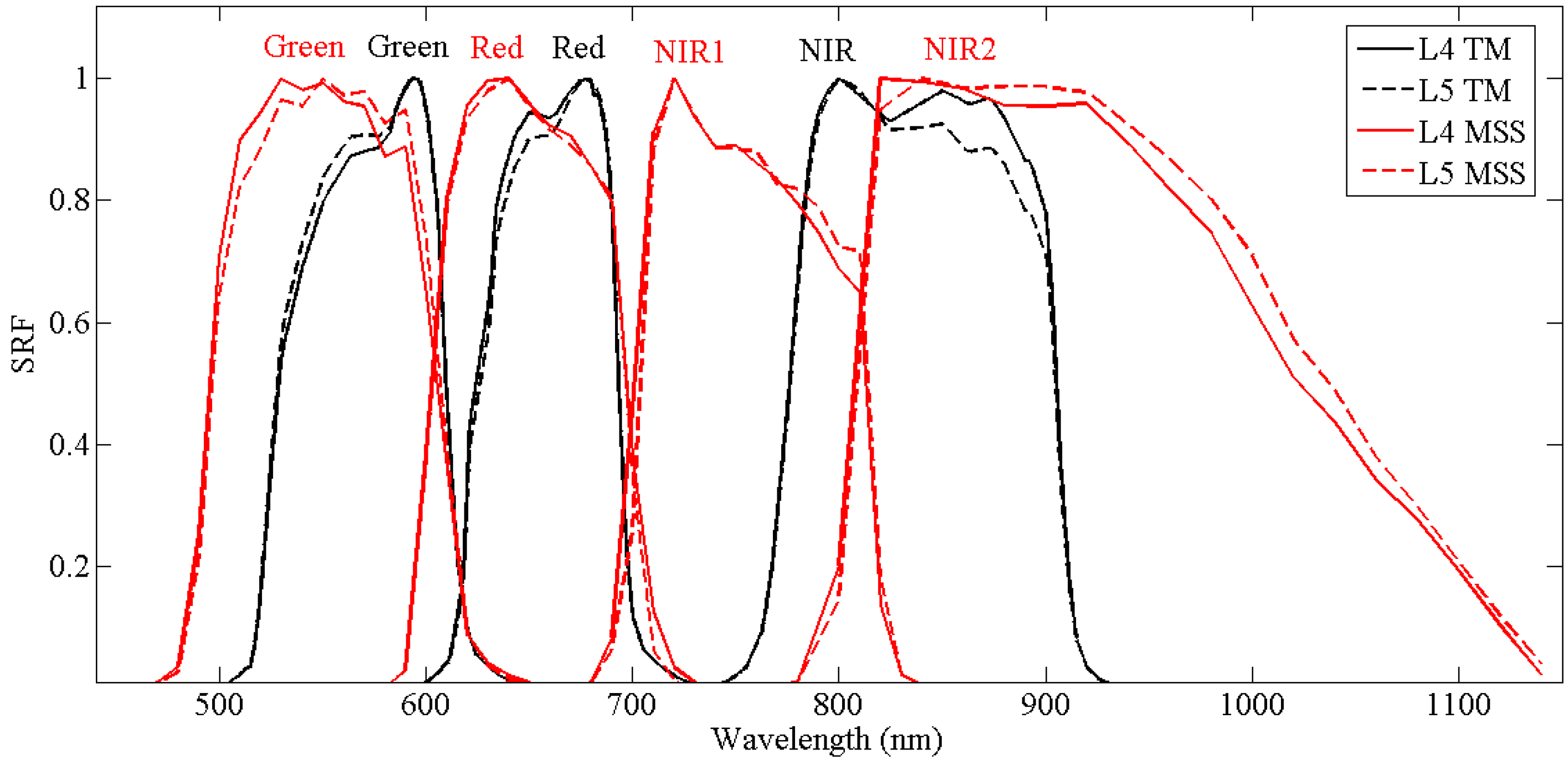
2.1. Spectral Response Function (SRF) of Landsat 4-5 MSS, TM, and Hyperion
2.2. Hyperion Spectra Collection
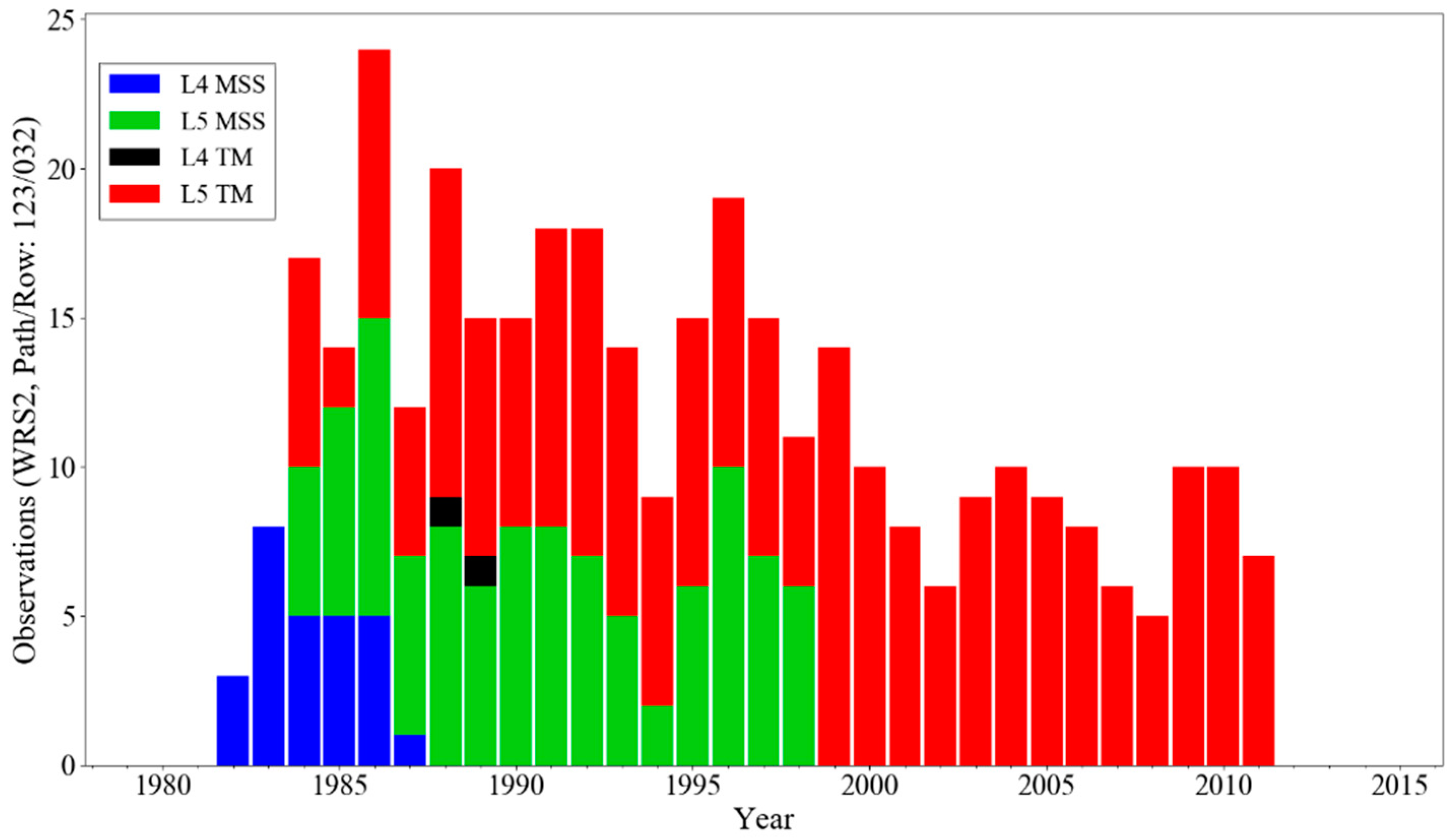
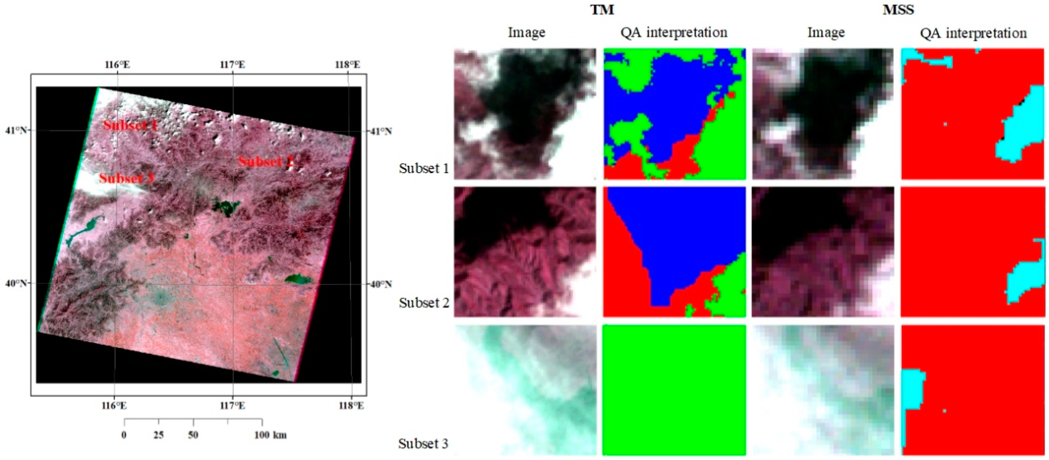
2.3. Paired MSS and TM Observations of Landsat 5 for Case Studies
2.4. Channel Reflectance Simulation
2.5. NDVI Estimation of the Landsat 4-5 MSS and TM
2.6. Between-Sensor Difference Measures
2.7. Transformation Models
3. Results
3.1. Intra-Platform Differences
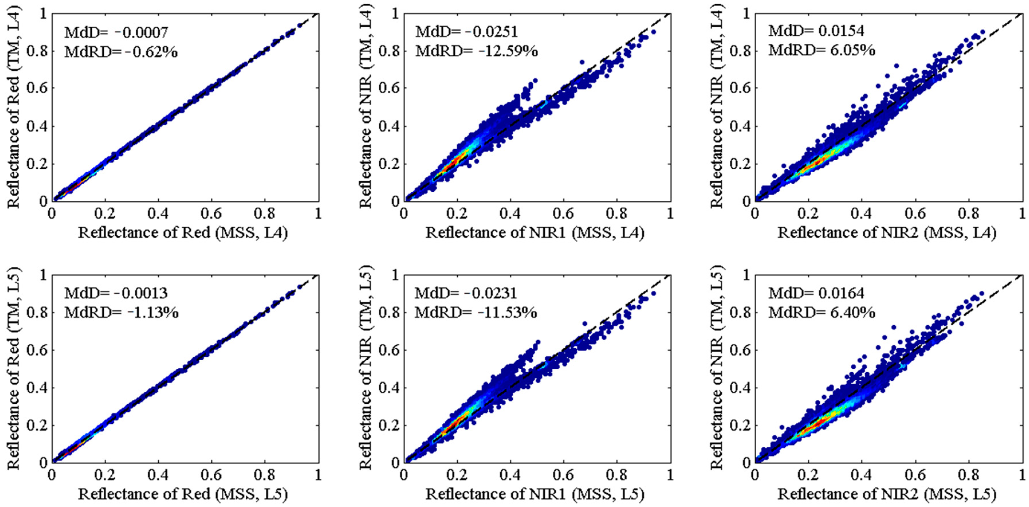
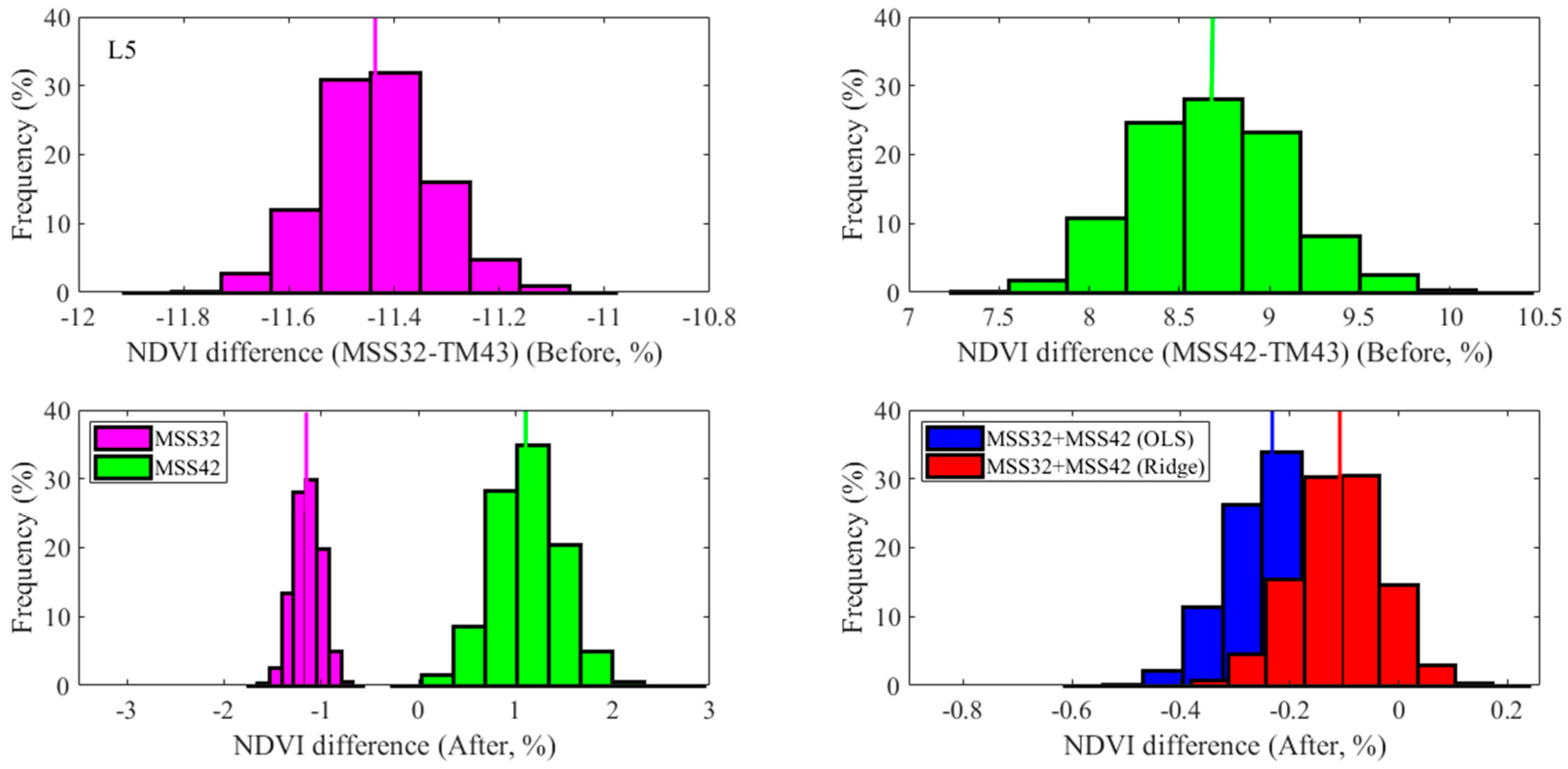
3.2. Inter-Platform Differences
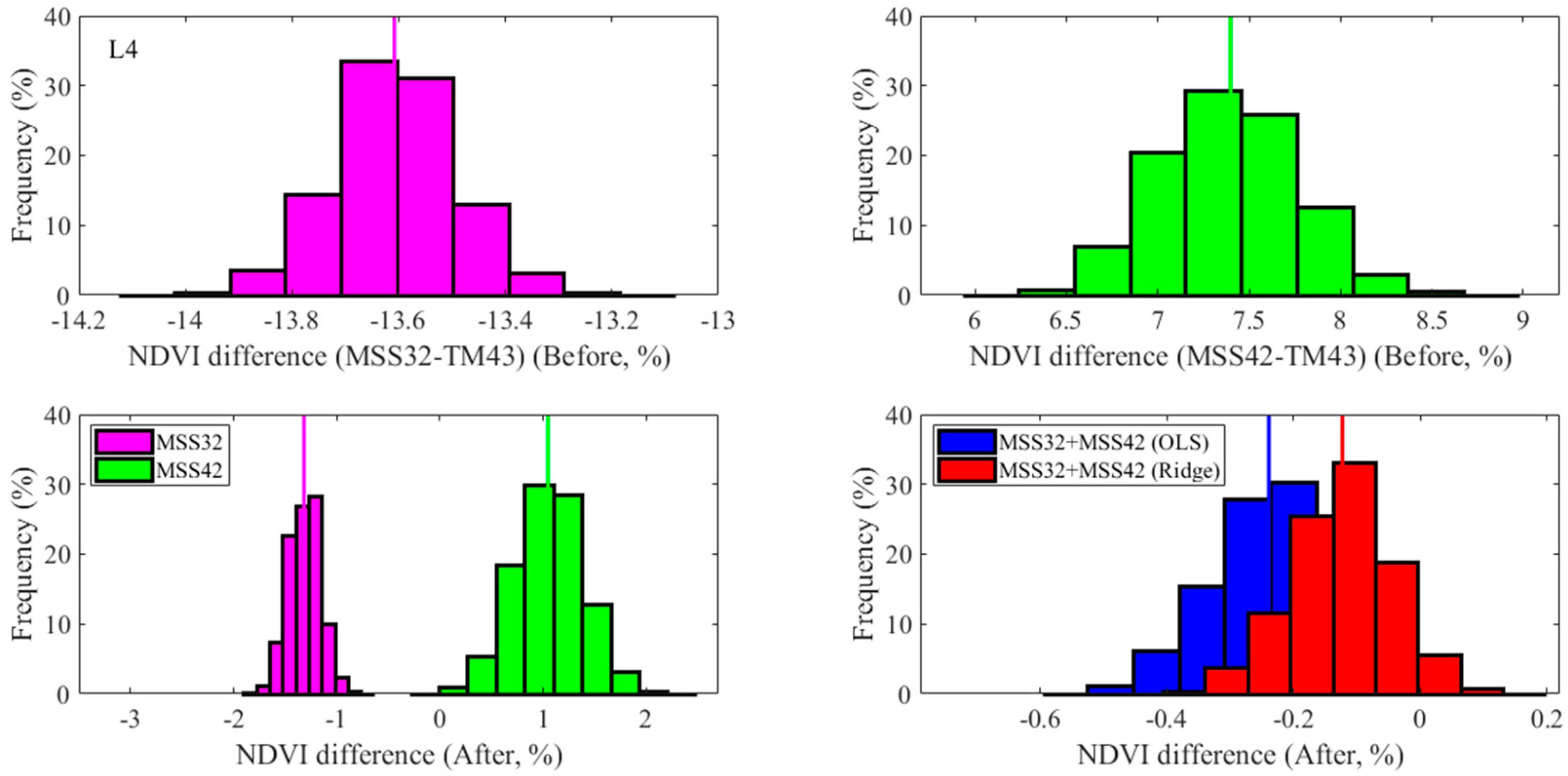
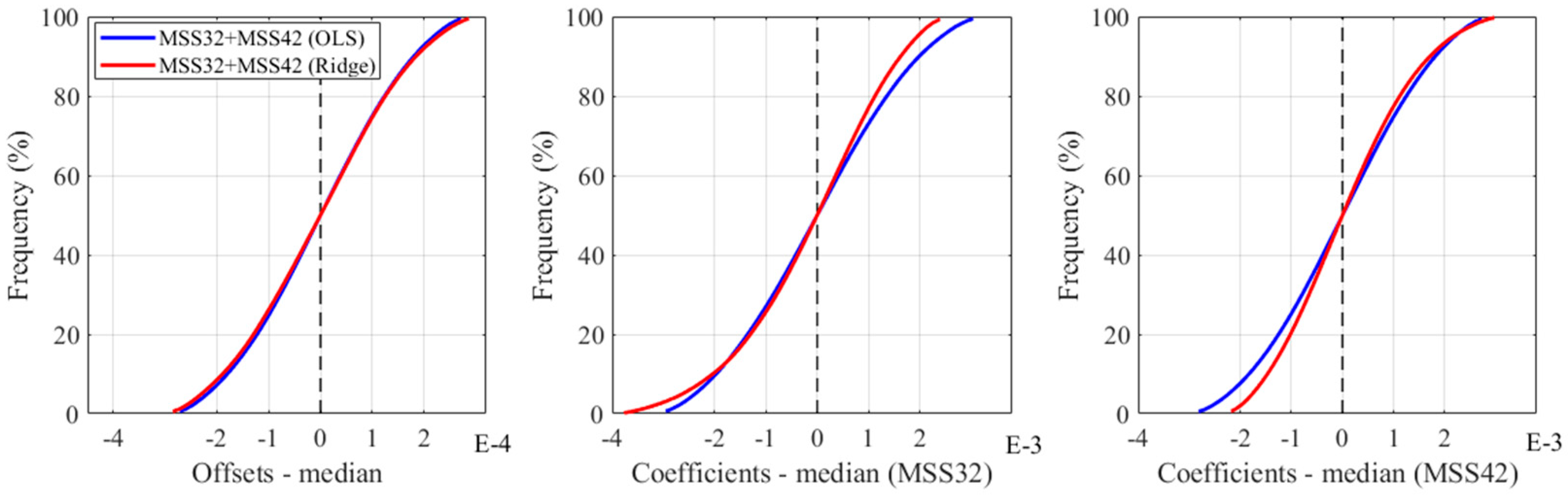
3.3. Transformation Models and Comparison
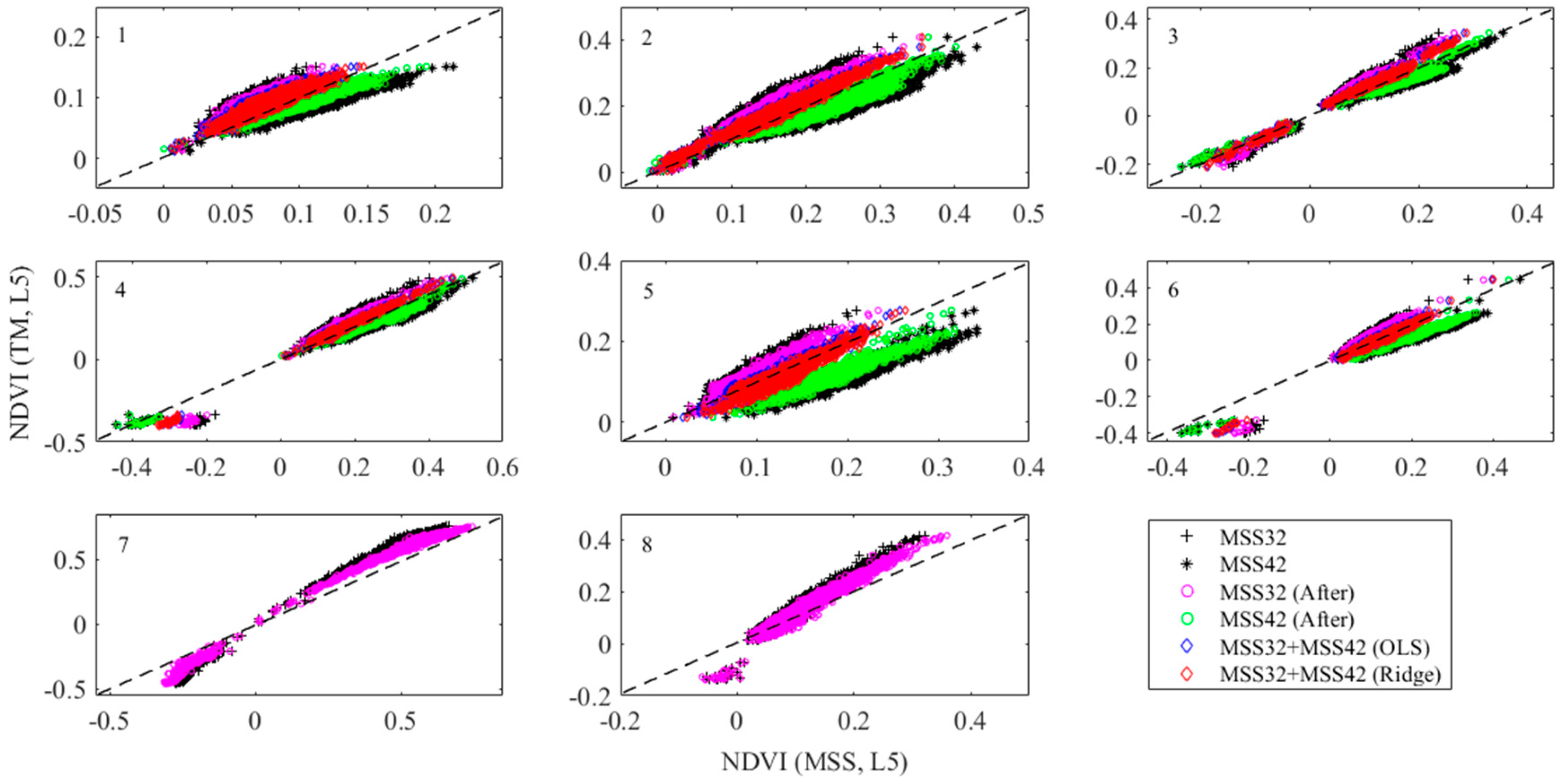
3.4. Application Cases
4. Discussion
4.1. Channel Reflectance Simulated from Hyperion Spectra
4.2. Transformation Modeling and Application
5. Conclusions
Author Contributions
Funding
Acknowledgments
Conflicts of Interest
References
- Woodcock, C.E.; Allen, R.; Anderson, M.; Belward, A.; Bindschadler, R.; Cohen, W.; Gao, F.; Goward, S.N.; Helder, D.; Helmer, E.; et al. Free access to Landsat imagery. Science 2008, 320, 1011. [Google Scholar] [CrossRef] [PubMed]
- Loveland, T.R.; Dwyer, J.L. Landsat: Building a strong future. Remote Sens. Environ. 2012, 122, 22–29. [Google Scholar] [CrossRef]
- Wulder, M.A.; White, J.C.; Loveland, T.R.; Woodcock, C.E.; Belward, A.S.; Cohen, W.B.; Fosnight, E.A.; Shaw, J.; Masek, J.G.; Roy, D.P. The global Landsat archive: Status, consolidation, and direction. Remote Sens. Environ. 2016, 185, 271–283. [Google Scholar] [CrossRef] [Green Version]
- Wulder, M.A.; Loveland, T.R.; Roy, D.P.; Crawford, C.J.; Masek, J.G.; Woodcock, C.E.; Allen, R.G.; Anderson, M.C.; Belward, A.S.; Cohen, W.B.; et al. Current status of Landsat program, science, and applications. Remote Sens. Environ. 2019, 225, 127–147. [Google Scholar] [CrossRef]
- Roy, D.P.; Kovalskyy, V.; Zhang, H.K.; Vermote, E.F.; Yan, L.; Kumar, S.S.; Egorov, A. Characterization of Landsat-7 to Landsat-8 reflective wavelength and normalized difference vegetation index continuity. Remote Sens. Environ. 2016, 185, 57–70. [Google Scholar] [CrossRef] [Green Version]
- Crist, E.P.; Cicone, R.C. Comparisons of the dimensionality and features of simulated Landsat-4 MSS and TM data. Remote Sens. Environ. 1984, 14, 235–246. [Google Scholar] [CrossRef]
- Haack, B.; Bryant, N.; Adams, S. An assessment of Landsat MSS and TM data for urban and near-urban land-cover digital classification. Remote Sens. Environ. 1987, 21, 201–213. [Google Scholar] [CrossRef]
- Khorram, S.; Brockhaus, J.A.; Cheshire, H.M. Comparison of Landsat MSS and TM data for urban land-use classification. IEEE Trans. Geosci. Remote Sens. 1987, GE-25, 238–243. [Google Scholar] [CrossRef]
- Price, J.C. Calibration comparison for the Landsat 4 and 5 multispectral scanners and thematic mappers. Appl. Opt. 1989, 28, 465–471. [Google Scholar] [CrossRef]
- Gallo, K.P.; Daughtry, C.S.T. Differences in vegetation indices for simulated Landsat-5 MSS and TM, NOAA-9 AVHRR, and SPOT-1 sensor systems. Remote Sens. Environ. 1987, 23, 439–452. [Google Scholar] [CrossRef]
- Renó, V.F.; Novo, E.M.; Suemitsu, C.; Rennó, C.D.; Silva, T.S. Assessment of deforestation in the Lower Amazon floodplain using historical Landsat MSS/TM imagery. Remote Sens. Environ. 2011, 115, 3446–3456. [Google Scholar] [CrossRef]
- Vittek, M.; Brink, A.; Donnay, F.; Simonetti, D.; Desclée, B. Land cover change monitoring using Landsat MSS/TM satellite image data over West Africa between 1975–1990. Remote Sens. 2014, 6, 658–676. [Google Scholar] [CrossRef]
- Lobo, F.L.; Costa, M.P.; Novo, E.M. Time-series analysis of Landsat-MSS/TM/OLI images over Amazonian waters impacted by gold mining activities. Remote Sens. Environ. 2015, 157, 170–184. [Google Scholar] [CrossRef]
- Fickas, K.C.; Cohen, W.B.; Yang, Z. Landsat-based monitoring of annual wetland change in the Willamette Valley of Oregon, USA from 1972 to 2012. Wetl. Ecol. Manag. 2016, 24, 73–92. [Google Scholar] [CrossRef]
- Markogianni, V.; Dimitriou, E. Landuse and NDVI change analysis of Sperchios river basin (Greece) with different spatial resolution sensor data by Landsat/MSS/TM and OLI. Desalin. Water Treat. 2016, 57, 29092–29103. [Google Scholar] [CrossRef]
- Savage, S.L.; Lawrence, R.L.; Squires, J.R.; Holbrook, J.D.; Olson, L.E.; Braaten, J.D.; Cohen, W.B. Shifts in forest structure in Northwest Montana from 1972 to 2015 using the Landsat archive from Multispectral Scanner to Operational Land Imager. Forests 2018, 9, 157. [Google Scholar] [CrossRef]
- Helder, D.L.; Karki, S.; Bhatt, R.; Micijevic, E.; Aaron, D.; Jasinski, B. Radiometric calibration of the Landsat MSS sensor series. IEEE Trans. Geosci. Remote Sens. 2012, 50, 2380–2399. [Google Scholar] [CrossRef]
- Sun, D.; Hu, C.; Qiu, Z.; Shi, K. Estimating phycocyanin pigment concentration in productive inland waters using Landsat measurements: A case study in Lake Dianchi. Opt. Express 2015, 23, 3055–3074. [Google Scholar] [CrossRef] [Green Version]
- Chen, F.; Yang, S.; Su, Z.; Wang, K. Effect of emissivity uncertainty on surface temperature retrieval over urban areas: Investigations based on spectral libraries. ISPRS J. Photogramm. Remote Sens. 2016, 114, 53–65. [Google Scholar] [CrossRef]
- Chen, F.; Yang, S.; Yin, K.; Chan, P. Challenges to quantitative applications of Landsat observations for the urban thermal environment. J. Environ. Sci. 2017, 59, 80–88. [Google Scholar] [CrossRef]
- Mohajane, M.; Essahlaoui, A.; Oudija, F.; El Hafyani, M.; El Hmaidi, A.; El Ouali, A.; Randazzo, G.; Teodoro, A.C. Land use/land cover (LULC) using Landsat data series (MSS, TM, ETM+ and OLI) in Azrou Forest, in the Central Middle Atlas of Morocco. Environments 2018, 5, 131. [Google Scholar] [CrossRef]
- USGS. Landsat Surface Reflectance-Derived Spectral Indices (Version 3.6). Available online: https://landsat.usgs.gov/sites/default/files/documents/si_product_guide.pdf (accessed on 15 April 2018).
- Claverie, M.; Ju, J.; Masek, J.G.; Dungan, J.L.; Vermote, E.F.; Roger, J.-C.; Skakun, S.V.; Justice, C. The Harmonized Landsat and Sentinel-2 surface reflectance data set. Remote Sens. Environ. 2018, 219, 145–161. [Google Scholar] [CrossRef]
- Barry, P.S.; Mendenhall, J.; Jarecke, P.; Folkman, M.; Pearlman, J.; Markham, B. EO-1 Hyperion hyperspectral aggregation and comparison with EO-1 Advanced Land Imager and Landsat 7 ETM+. In Proceedings of the IEEE 2002 International Geoscience and Remote Sensing Symposium, Toronto, ON, Canada, 24–28 June 2002; pp. 1648–1651. [Google Scholar]
- Chander, G.; Mishra, N.; Helder, D.L.; Aaron, D.B.; Angal, A.; Choi, T.; Xiong, X.; Doelling, D.R. Applications of spectral band adjustment factors (SBAF) for cross-calibration. IEEE Trans. Geosci. Remote Sens. 2013, 51, 1267–1281. [Google Scholar] [CrossRef]
- Chen, F.; Lou, S.L.; Fan, Q.C.; Li, J.; Wang, C.; Claverie, M. A preliminary investigation on comparison and transformation of Sentinel-2 MSI and Landsat 8 OLI. Int. Arch. Photogramm. Remote Sens. Spat. Inf. Sci. 2018, XLII-3, 2619–2624. [Google Scholar] [CrossRef]
- Wen, Z.F.; Zhang, S.Q.; Wu, S.J.; Liu, F.; Jiang, Y. Evaluating the consistency of multi-source wideband remote sensing images: A band simulation approach using Hyperion data. J. Remote Sens. 2013, 17, 1533–1545. [Google Scholar] [CrossRef]
- Ungar, S.G.; Middleton, E.M.; Ong, L.; Campbell, P.K. EO-1 Hyperion Onboard Performance over Eight Years: Hyperion Calibration. In Proceedings of the 6th EARSeL Imaging Spectroscopy SIG Workshop, Tel Aviv, Israel, 16–19 March 2009; pp. 1–6. [Google Scholar]
- Folkman, M.A.; Pearlman, J.; Liao, L.B.; Jarecke, P.J. EO-1/Hyperion hyperspectral imager design, development, characterization, and calibration. Proc. SPIE 2001, 4151, 40–51. [Google Scholar]
- Czapla-Myers, J.; Ong, L.; Thome, K.; McCorkel, J. Validation of EO-1 Hyperion and Advanced Land Imager using the radiometric calibration test site at Railroad Valley, Nevada. IEEE J. Sel. Top. Appl. 2016, 9, 816–825. [Google Scholar] [CrossRef]
- Claverie, M.; Masek, J.G.; Ju, J.; Dungan, J.L. Harmonized Landsat-8 Sentinel-2 (HLS) Product User’s Guide. Available online: https://hls.gsfc.nasa.gov/documents/ (accessed on 15 April 2018).
- Helder, D.L.; Thome, K.J.; Mishra, N.; Chander, G.; Xiong, X.; Angal, A.; Choi, T. Absolute radiometric calibration of Landsat using a pseudo invariant calibration site. IEEE Trans. Geosci. Remote Sens. 2013, 51, 1360–1369. [Google Scholar] [CrossRef]
- Pinto, C.T.; Ponzoni, F.J.; Castro, R.M.; Leigh, L.; Kaewmanee, M.; Aaron, D.; Helder, D. Evaluation of the uncertainty in the spectral band adjustment factor (SBAF) for cross-calibration using Monte Carlo simulation. Remote Sens. Lett. 2016, 7, 837–846. [Google Scholar] [CrossRef]
- Hu, K.; Chen, F.; Liang, S.W. Application of HJ-1B data in monitoring water surface temperature. Proc. Environ. Sci. 2011, 10, 2042–2049. [Google Scholar] [CrossRef]
- Chen, F.; Yang, S.; Su, Z.; He, B.Y. A new single-channel method for estimating land surface temperature based on the image inherent information: The HJ-1B case. ISPRS J. Photogramm. Remote Sens. 2015, 101, 80–88. [Google Scholar] [CrossRef]
- Tucker, J.C. Red and photographic infrared linear combination for monitoring vegetation. Remote Sens. Environ. 1979, 8, 127–150. [Google Scholar] [CrossRef]
- Xiong, Y.Z.; Huang, S.P.; Chen, F.; Ye, H.; Wang, C.P.; Zhu, C.B. The impacts of rapid urbanization on the thermal environment: A remote sensing study of Guangzhou, South China. Remote Sens. 2012, 4, 2033–2056. [Google Scholar] [CrossRef]
- Pan, F.; Xie, J.; Lin, J.; Zhao, T.; Ji, Y.; Hu, Q.; Pan, X.; Wang, C.; Xi, X. Evaluation of climate change impacts on wetland vegetation in the Dunhuang Yangguan National Nature Reserve in Northwest China using Landsat derived NDVI. Remote Sens. 2018, 10, 735. [Google Scholar] [CrossRef]
- Li, D.; Lu, D.; Wu, M.; Shao, X.; Wei, J. Examining land cover and greenness dynamics in Hangzhou Bay in 1985–2016 using Landsat time-series data. Remote Sens. 2018, 10, 32. [Google Scholar] [CrossRef]
- Flood, N. Continuity of reflectance data between Landsat-7 ETM+ and Landsat-8 OLI, for both top-of-atmosphere and surface reflectance: A study in the Australian Landscape. Remote Sens. 2014, 6, 7952–7970. [Google Scholar] [CrossRef]
- Fan, X.W.; Liu, Y.B. Multisensor normalized difference vegetation index intercalibration: A comprehensive overview of the causes of and solutions for multisensor differences. IEEE Geosci. Remote Sens. Mag. 2018, 6, 23–45. [Google Scholar] [CrossRef]
- Li, P.; Jiang, L.; Feng, Z. Cross-comparison of vegetation indices derived from Landsat-7 Enhanced Thematic Mapper Plus (ETM+) and Landsat-8 Operational Land Imager (OLI) sensors. Remote Sens. 2014, 6, 310–329. [Google Scholar] [CrossRef]
- Hoerl, A.E.; Kennard, R.W. Ridge regression: Biased estimation for nonorthogonal problems. Technometrics 2000, 42, 80–86. [Google Scholar] [CrossRef]
- Gorroño, J.; Banks, A.C.; Fox, N.P.; Underwood, C. Radiometric inter-sensor cross-calibration uncertainty using a traceable high accuracy reference hyperspectral imager. ISPRS J. Photogramm. Remote Sens. 2017, 130, 393–417. [Google Scholar] [CrossRef] [Green Version]
- Jia, G.; Hueni, A.; Tao, D.; Geng, R.; Schaepman, M.E.; Zhao, H. Spectral super-resolution reflectance retrieval from remotely sensed imaging spectrometer data. Opt. Express 2016, 24, 19905–19919. [Google Scholar] [CrossRef] [PubMed]
- Chander, G.; Markham, B.L.; Helder, D.L. Summary of current radiometric calibration coefficients for Landsat MSS, TM, ETM+, and EO-1 ALI sensors. Remote Sens. Environ. 2009, 113, 893–903. [Google Scholar] [CrossRef]
- Zhang, H.K.; Roy, D.P.; Yan, L.; Li, Z.; Huang, H.; Vermote, E.; Skakun, S.; Roger, J.C. Characterization of Sentinel-2A and Landsat-8 top of atmosphere, surface, and nadir BRDF adjusted reflectance and NDVI differences. Remote Sens. Environ. 2018, 215, 482–494. [Google Scholar] [CrossRef]
- Ke, Y.; Im, J.; Lee, J.; Gong, H.; Ryu, Y. Characteristics of Landsat 8 OLI-derived NDVI by comparison with multiple satellite sensors and in-situ observations. Remote Sens. Environ. 2015, 164, 298–313. [Google Scholar] [CrossRef]
- Claverie, M.; Vermote, E.F.; Franch, B.; Masek, J.G. Evaluation of the Landsat-5 TM and Landsat-7 ETM+ surface reflectance products. Remote Sens. Environ. 2015, 169, 390–403. [Google Scholar] [CrossRef]
- Vogelmann, J.E.; Gallant, A.L.; Shi, H.; Zhu, Z. Perspectives on monitoring gradual change across the continuity of Landsat sensors using time-series data. Remote Sens. Environ. 2016, 185, 258–270. [Google Scholar] [CrossRef] [Green Version]


| MSS | TM | |
|---|---|---|
| Blue | -- | B1: 450–520 nm (30 m) |
| Green | B1: 500–600 nm (60 m) | B2: 520–600 nm (30 m) |
| Red | B2: 600–700 nm (60 m) | B3: 630–690 nm (30 m) |
| NIR | B3 (NIR1): 700–800 nm (60 m) B4 (NIR2): 800–11000 nm (60 m) | B4: 760–900 nm (30 m) -- |
| SWIR | -- -- | B5: 1550–1750 nm (30 m) B7: 2080–2350 nm (30 m) |
| Thermal infrared | -- | B6: 10.40–12.50 μm (120 m 1) |
| Case | Landsat 5 MSS | Landsat 5 TM |
|---|---|---|
| 1 | LM05_L1TP_123032_19850312_20180405_01_T2 | LT05_L1TP_123032_19850312_20170219_01_T1 |
| 2 | LM05_L1TP_123032_19851022_20180407_01_T2 | LT05_L1TP_123032_19851022_20170218_01_T1 |
| 3 | LM05_L1TP_123032_19880421_20180326_01_T2 | LT05_L1TP_123032_19880421_20170221_01_T1 |
| 4 | LM05_L1TP_123032_19881014_20180327_01_T2 | LT05_L1TP_123032_19881014_20170206_01_T1 |
| 5 | LM05_L1TP_123032_19900105_20180323_01_T2 | LT05_L1TP_123032_19900105_20170201_01_T1 |
| 6 | LM05_L1TP_123032_19901121_20180324_01_T2 | LT05_L1TP_123032_19901121_20180620_01_T1 |
| 7 | LM05_L1TP_123032_19950916_20180315_01_T2 | LT05_L1TP_123032_19950916_20170107_01_T1 |
| 8 | LM05_L1TP_123032_19951221_20180315_01_T2 | LT05_L1TP_123032_19951221_20170106_01_T1 |
| MSS42(L4) | MSS32(L4) | TM43(L4) | MSS42(L5) | MSS32(L5) | TM43(L5) | |
|---|---|---|---|---|---|---|
| MSS42(L4) | -- | 0.9870 | 0.9908 | 1.0000 | 0.9870 | 0.9907 |
| MSS32(L4) | 24.39% | -- | 0.9981 | 0.9868 | 1.0000 | 0.9981 |
| TM43(L4) | 7.40% | −13.61% | -- | 0.9907 | 0.9981 | 1.0000 |
| MSS42(L5) | −0.84% | −21.16% | −8.13% | -- | 0.9868 | 0.9905 |
| MSS32(L5) | 21.79% | −2.12% | 13.09% | 22.81% | -- | 0.9982 |
| TM43(L5) | 7.79% | −13.32% | 0.42% | 8.68% | −11.44% | -- |
| Intra-Platform Transformation | MSE1 | MdD | MdRD | |
| L4 OLS | TM43 = 0.0012 + 1.1380MSS32 | 0.0213 | −0.0032 | −1.32% |
| OLS | TM43 = −0.0106 + 0.9703MSS42 | 0.0379 | 0.0008 | 1.04% |
| OLS | TM43 = −0.0065 + 0.7724MSS32 + 0.3226MSS42 | 0.0123 | −0.0006 | −0.24% |
| Ridge | TM43 = −0.0051 + 0.7023MSS32 + 0.3767MSS42 | 0.0128 | −0.0003 | −0.12% |
| L5 OLS | TM43 = −0.0006 + 1.1181MSS32 | 0.0198 | −0.0028 | −1.15% |
| OLS | TM43 = −0.0116 + 0.9628MSS42 | 0.0390 | −0.0010 | −1.11% |
| OLS | TM43 = −0.0076 + 0.7888MSS32 + 0.2939MSS42 | 0.0118 | −0.0006 | −0.23% |
| Ridge | TM43 = −0.0064 + 0.7097MSS32 + 0.3564MSS42 | 0.0124 | −0.0003 | −0.10% |
| Inter-Platform Transformation (L4 to L5) | MSE | MdD | MdRD | |
| OLS | TM43(L5) = −0.0011 + 1.0001TM43(L4) | 0.0007 | 0.00002 | 0.02% |
| OLS | TM43 = 0.0001 + 1.1384MSS32 | 0.0208 | −0.0032 | −1.30% |
| OLS | TM43 = −0.0115 + 0.9701MSS42 | 0.0384 | −0.0008 | 1.08% |
| OLS | TM43 = −0.0074 + 0.7845MSS32 + 0.3122MSS42 | 0.0122 | −0.0007 | −0.26% |
| Ridge | TM43 = −0.0061 + 0.7102MSS32 + 0.3699MSS42 | 0.0127 | −0.0003 | −0.12% |
| MSS32 | MSS42 | MSS32 (After) | MSS42 (After) | MSS32+MSS42 (OLS) | MSS32+MSS42 (Ridge) | ||
|---|---|---|---|---|---|---|---|
| 1 | MdD | −0.0303 | 0.0223 | −0.0233 | 0.0064 | −0.0170 | −0.0135 |
| MdRD | −32.27% | 24.02% | −24.91% | 6.91% | −18.30% | −14.59% | |
| 2 | MdD | −0.0523 | 0.0427 | −0.0391 | 0.0230 | −0.0224 | −0.0172 |
| MdRD | −30.70% | 25.06% | −22.90% | 13.51% | −13.02% | −9.96% | |
| 3 | MdD | −0.0486 | 0.0440 | −0.0382 | 0.0255 | −0.0215 | −0.0161 |
| MdRD | −34.46% | 31.12% | −27.14% | 18.02% | −15.30% | −11.45% | |
| 4 | MdD | −0.0524 | 0.0398 | −0.0398 | 0.0207 | −0.0240 | −0.0189 |
| MdRD | −31.81% | 24.46% | −24.12% | 12.71% | −14.51% | −11.45% | |
| 5 | MdD | −0.0202 | 0.0782 | −0.0115 | 0.0600 | 0.0074 | 0.0135 |
| MdRD | −20.39% | 78.31% | −11.58% | 59.74% | 7.41% | 13.50% | |
| 6 | MdD | −0.0306 | 0.0738 | −0.0212 | 0.0552 | −0.0008 | 0.0055 |
| MdRD | −26.43% | 62.73% | −18.25% | 46.75% | −0.70% | 4.70% | |
| 7 | MdD | −0.1131 | -- | −0.0508 | -- | -- | -- |
| MdRD | −18.14% | -- | −8.57% | -- | -- | -- | |
| 8 | MdD | −0.0205 | -- | −0.0117 | -- | -- | -- |
| MdRD | −20.53% | -- | −11.74% | -- | -- | -- |
© 2019 by the authors. Licensee MDPI, Basel, Switzerland. This article is an open access article distributed under the terms and conditions of the Creative Commons Attribution (CC BY) license (http://creativecommons.org/licenses/by/4.0/).
Share and Cite
Chen, F.; Lou, S.; Fan, Q.; Wang, C.; Claverie, M.; Wang, C.; Li, J. Normalized Difference Vegetation Index Continuity of the Landsat 4-5 MSS and TM: Investigations Based on Simulation. Remote Sens. 2019, 11, 1681. https://doi.org/10.3390/rs11141681
Chen F, Lou S, Fan Q, Wang C, Claverie M, Wang C, Li J. Normalized Difference Vegetation Index Continuity of the Landsat 4-5 MSS and TM: Investigations Based on Simulation. Remote Sensing. 2019; 11(14):1681. https://doi.org/10.3390/rs11141681
Chicago/Turabian StyleChen, Feng, Shenlong Lou, Qiancong Fan, Chenxing Wang, Martin Claverie, Cheng Wang, and Jonathan Li. 2019. "Normalized Difference Vegetation Index Continuity of the Landsat 4-5 MSS and TM: Investigations Based on Simulation" Remote Sensing 11, no. 14: 1681. https://doi.org/10.3390/rs11141681