1. Introduction
Synthetic Aperture Radar (SAR) imaging aims to characterize the interaction of the transmitted electromagnetic waves with scatterers in the imaged scene. In practice, the recorded SAR raw data do describe these interactions but also include a multitude of effects that are due to the SAR sensor hardware and the propagation of signals within it. These systematic, sensor induced effects are not related to the contents of the imaged scene and hinder a meaningful interpretation of the resulting imagery. Such issues are especially relevant in the case of advanced SAR sensors, with analog or even digital beam-forming (DBF), that employ antenna arrays: systematic errors at the level of the individual antenna array element will impair or even prohibit image formation itself, as the effective antenna illumination patterns will deviate from the expectation and lead to errors in SAR focusing.
The continued interest in scientific and operational exploitation of SAR in a diverse set of remote sensing applications has lead to ever more stringent requirements regarding the calibration quality of SAR data delivered by modern sensors. At the same time, SAR sensors are becoming more complex and consequently more difficult to calibrate. This is especially true for new SAR imaging modes that involve simultaneous data acquisition in multiple channels for polarimetric imaging, single-pass interferometry or DBF. The task of SAR sensor calibration is therefore becoming simultaneously more important from an application point of view and more difficult in view of the underlying sensor complexity.
This is especially true for airborne SAR sensors for research, which play an important role in the process of SAR sensor development and are often technological precursors of the next generation of satellite SAR sensors. The DLR’s Microwaves and Radar Institute currently operates several airborne SAR sensors that cover a wide range of innovative imaging techniques, including polarimetric imaging, single-pass polarimetric multi-baseline interferometry and multi-channel along-track interferometry. This paper details a general calibration approach that was developed to meet the diverse requirements implied by these multi-channel SAR imaging modes. As such, the approach necessarily entails multiple steps that address calibration issues related to imaging geometry, radiometry and the polarimetric/interferometric inter-channel phase difference.
SAR sensor calibration generally involves both internal calibration and external calibration [
1]. Internal calibration is based on measurements performed internally by the SAR sensor. These can later be used to correct for distortions and transient drifts when radar pulses are transmitted or received.
The discussion in this paper takes the internal calibration as a given and is mainly concerned with aspects of SAR sensor calibration that are outside the scope of internal measurements. These aspects make up the external sensor calibration, in which actual SAR measurements of reference targets with known properties are analyzed to refine an existing sensor model. These refinements are primarily concerned with the multi-aperture antenna array of the multi-channel SAR sensor under consideration.
The relevant properties of reference targets, such as position, size and orientation, among others, must be well known such that the targets’ expected radar return can be predicted with a high degree of accuracy for any given imaging geometry. External sensor calibration is then the process of estimating corrections to eliminate systematic deviations of the measured target response from the a priori expectation.
The calibration technique discussed in this paper differs from existing techniques in that it is based entirely on range compressed raw data, instead of relying on the analysis of focused SAR imagery. The novelty lies in analyzing the response of reference targets in a pulse-by-pulse fashion, such that additional information concerning the variation of key quantities within the illumination time of each target can be leveraged in the estimation of propagation direction dependent calibration corrections.
As will be argued in the next section, this approach is especially suited in the context of multi-channel SAR and DBF. A more general advantage of basing the calibration directly on raw data, rather than focused imagery, is that it ensures independence from the SAR processor. Modern SAR processors are highly complex and it is often difficult to distinguish calibration issues that arise at the sensor level from errors introduced by the processor in focusing the SAR imagery. Decoupling the processor from the task of calibration reduces complexity and can help pinpoint issues in the SAR processor. Calibration results do not transfer to the focused SAR imagery as expected in the presence of processing artifacts.
The remainder of the paper is organized as follows:
Section 2 provides an overview of the state of the art in external SAR sensor calibration and indicates the contributions of the proposed approach.
Section 3 introduces the reference target response model used and describes how the SAR data in calibration acquisitions are analyzed to quantify any mismatch between the measured and the expected target response.
Section 4 describes how a rigorous optimization process connects the measured response mismatch to appropriate calibration corrections, while
Section 5 illustrates and validates the approach using real multi-channel SAR data and finally
Section 6 concludes the paper.
2. State of the Art
A number of recent satellite SAR missions have involved extensive, well-documented and highly successful external calibration programs. Representative examples include the approaches developed for the TerraSAR-X [
2] and TanDEM-X [
3] missions, launched in 2007 and 2010, respectively, as well as the Cosmo-Skymed mission [
4], with four satellites launched between 2007 and 2010, the Sentinel-1 mission [
5], with satellites A and B launched in 2014 and 2016, respectively, and the Radarsat-2 mission [
6]. Similar techniques have also been applied for the calibration of airborne SAR sensors, such the F-SAR sensor operated by the German Aerospace Center (DLR) [
7,
8].
All of the above satellite missions feature highly complex radar instruments with phased-array antennas consisting of hundreds of individually controlled antenna elements to support advanced SAR imaging modes. Different imaging modes are facilitated by beam-forming techniques that combine signals from multiple antenna elements within the instrument. Here, amplitude and phase adjustments to individual signals change the effective antenna diagram while data are being acquired.
This type of SAR sensor represents a considerable challenge in terms of calibration due to the large configuration space required to support a variety of imaging modes. In the case of the TerraSAR-X and TanDEM-X sensors, for instance, the operational imaging modes are defined in terms of more than 10,000 unique effective antenna patterns [
9] (also known as ‘beams’). Due to limited resources, in terms of time during the sensor commissioning phase and budget, it is neither possible nor desirable to attempt the individual characterization and calibration of these beams on the basis of SAR measurements acquired after the sensor has been deployed in orbit. Instead, large parts of the calibration effort are based on an antenna model [
9,
10] that is able to accurately reproduce the effective antenna illumination pattern given the settings applied at the level of the individual antenna array element. This model can then be validated by comparing its predictions with actual SAR measurements for a comparatively tiny number of beams. Once validated, it is assumed to generalize to all other beams employed during operational data acquisition and may be relied upon to provide the detailed, propagation direction dependent antenna characterization that is used to compensate for systematic antenna-related effects during SAR data processing.
A major focus of external calibration activities in the context of modern SAR missions is therefore the validation of the antenna model. Studies [
9] and [
11] outline the external validation of the antenna models used for the TerraSAR-X and Sentinel-1A SAR instruments, respectively. Similar calibration approaches have been used for the COSMO-SkyMed [
12] and Radarsat-2 [
13] instruments. These approaches are similar and comprise a set of techniques to assess the antenna diagrams in elevation and azimuth and estimate the antenna mispointing. Focused SAR imagery acquired over areas of homogeneous backscatters, typically the Amazon rain forest, are used to validate the elevation antenna diagram and estimate the elevation mispointing. The later estimate uses dedicated acquisitions employing a
notch antenna pattern. In azimuth, meanwhile, the validation of the diagram and the mispointing estimate are based on active calibration targets [
14]. For polarimetric sensors, acquisitions with active targets can also be used for polarimetric cross-talk calibration [
15].
In addition to antenna model validation, external calibration also entails the estimation calibration constants that account for constant offsets in gain, delay and phase that are mainly due to propagation effects within the instrument. These constants are estimated using reference targets with known properties, such that their expected response in SAR acquisitions can be predicted accurately. The analysis of reference target returns is carried out in focused SAR imagery of point-like targets [
1,
16], such as radar reflectors or specifically selected distributed targets, such as water surfaces [
17].
Notwithstanding the success and proven accuracy of established calibration techniques, the approach presented in the following sections may offer certain advantages in the context of multi-channel SAR systems. Firstly, conventional external calibration techniques rely heavily on focused SAR imagery. In addition to the arguably undesirable reliance on SAR processing software, the use of focused imagery may not even be an option for multi-channel systems that require analog or digital beam-forming techniques, in range or in azimuth, carried out on board or on ground, for image formation. For such instruments, image formation supposes a well-calibrated antenna array but calibration requires image formation. The present approach circumvents this circular problem, as it does not require SAR image formation and can be applied to data that are under-sampled in azimuth. Similarly, it can be applied without modification in arbitrary imaging geometries, such as circular SAR [
18], or to data that is irregularly sampled in azimuth [
19].
Secondly, existing approaches are geared towards verifying an existing antenna model. They do not, generally, include mechanisms to systematically work backwards from an observed mismatch between expectation and observation to a set of causes for the mismatch and the corresponding corrections. The proposed approach introduces explicit error models and derives corrections through a rigorous optimization process. In particular, it explicitly addresses uncertainty in the three dimensional antenna phase center positions to ensure the consistent inter-channel phase and geometry that are of central importance in most multi-channel SAR applications. Furthermore, the optimization approach naturally lends itself to a more detailed modeling of error sources. For instance, the proposed antenna mispointing estimate can derive three dimensional roll/pitch/yaw corrections, rather than the conventional elevation/azimuth estimates. It can also provide separate corrections for the transmit and receive channels when these involve different antennas.
3. Target Response Model and Analysis
As outlined in
Figure 1, the proposed external calibration workflow starts with the analysis of reference target responses in multiple channels of acquired SAR data. The analysis is repeated throughout the calibration process to take into account each calibration correction as it becomes available.
The notation adopted throughout the following sections uses to denote the azimuth sample index and super- and sub-scripts to indicate any quantity derived from the response of reference target s in a SAR data channel that uses the antenna elements p and q on transmit and receive, respectively. An antenna element is, for the present purposes, the smallest constituent of an antenna array that can individually send and/or receive signals. In particular, polarimetric antennas are considered as two independent elements corresponding to the horizontal and vertical polarizations.
The calibration approach is intended to be applied to a data set comprising one or more calibration data acquisitions. Such acquisitions contain reference targets that are imaged over a wide range of off-nadir angles. To avoid unnecessary complication of the notations adopted, the reference target superscript s is specific to the data acquisition. Thus, when the same target appears in independent acquisitions, the responses are treated as though originating from different targets.
3.1. Acquisition Geometry and Response Model
External calibration entails the comparison of the measured target response with the expectation. The expected response depends on sensor and target properties, but also on the acquisition geometry. For the purposes of calibration, it is convenient to describe the geometry in a rest frame of the instrument. This frame is a Cartesian coordinate system that translates and rotates with the sensor platform. A fixed point
in a global coordinate system transforms into a time-variant coordinate
in the instrument coordinate system as
where
is the position of the instrument reference point in global coordinates, as measured by the navigation subsystem, and
denotes the rotation into the rest frame and depends on the time variant sensor attitude angles.
In instrument coordinates, the phase centre of an antenna element is constant and is given by the sum of and . These former represents the assumed phase center position. The latter denotes the correction to this position introduced in the process of sensor calibration. It is initially assumed to be zero.
The position of the target
is obtained from the known global target coordinate via the transform (
1). The position of the target relative to a phase centre
e is then defined as
where
is the channel dependent mapping from azimuth sample index
onto the continuous time axis
t. Note that this formulation assumes that the
start-stop effect can be ignored, as is the case for airborne SAR but not for spaceborne platforms and high spatial resolutions [
20].
Normalizing the relative position of the target gives the azimuth variant line of sight (LOS) vectors towards the target:
In a given acquisition geometry, the expected target response
varies as a function of the azimuth sample index
and the physical range frequency
. This response has an amplitude that is closely related to the radar equation for real aperture radar [
21] as well as a phase related to the spatial seperation of sensor and target. The combination of these terms is the response model underlying the calibration process:
where
c is the speed of light and
j denotes
.
The phase of the reference target response is related to the target range and can be written as
where
is a tropospheric propagation delay correction that is introduced in the calibration process and is initially assumed zero.
The power of the response, meanwhile, is given by the received signal power as defined in the context of the radar equation for real aperture radar [
21]. It includes the free space propagation loss in the denominator as well as the azimuth variant antenna amplification
and the target backscatter amplitude
. The antenna amplification is given by
where
is the complex valued antenna diagram of element
e, which is a function of propagation direction (angles
and
) and frequency
. These per-element diagrams are assumed known. They will typically have been derived from the precise on-ground characterization of the antenna array [
22]. The power of the complex diagram is the antenna gain.
The azimuth variant propagation direction towards the target is defined in the so-called
element coordinate system, which is related to the instrument coordinate system by a rotation
. The rotation accounts for, and is defined in terms of, the
antenna element mount angles
which represent the mispointing of each antenna element
e. These angles are initially unknown and assumed zero.
The expected target backscatter amplitude is accounted for in a similar fashion to the antenna pattern. The target amplitude varies as a function of the azimuth-variant propagation direction towards the sensor. It also depends on the polarization state of the transmit and receive antenna elements and varies as a function of the range frequency. It may also be complex valued if the reference target is known to be not an ideal point-like scatterer. The power of the modeled target backscatter is the radar cross section in .
The backscatter model of each target is assumed known and may be directly measured, derived from electromagnetic simulations or analytically from geometric optics [
23]. In addition to the backscatter model, the computation of
requires geometric transforms into a suitable reference target coordinate system. This coordinate system is the analog of the antenna element coordinate system introduced above. Details of the model used and the coordinate systems adopted are, however, beyond the scope of this article.
3.2. Response Analysis
To provide the inputs required for estimating calibration corrections, the measured target response is compared to the expected target response of (
4), as illustrated in
Figure 2. Any systematic discrepancy is potentially a sensor calibration issue that should be addressed by estimating corresponding calibration corrections. Such discrepancies will be termed residual errors in the following.
For a given data channel that uses antenna elements
p and
q to transmit and receive echos, respectively, the sensor acquires a 2D echo buffer
defined over range and azimuth sample indices
and
, respectively. The normalized response of a target
s is closely related to residual errors in the response. It is given by
where
and
denote the forward and inverse discrete Fourier transform, respectively.
is the expected target response, defined in terms of the physical range frequency
in (
4), while
is a correction derived from the composition of internal calibration measurements and external calibration corrections:
In the above, is a 2D buffer of internal calibration pulses recorded alongside the data channel in question. In practice, the SAR sensor might not record an internal calibration signal for each and every pulse. The calibration buffer would then have to be interpolated in azimuth. Alternatively, internal calibration information may not be acquired during the actual data take at all. In this case, the calibration signal takes the form of a 1D chirp replica that is constant over azimuth. , meanwhile, is a one dimensional, complex valued correction to the range frequency response. This correction is initially unknown and assumed equal to unity until estimates become available during the calibration process.
The application of Equation (
8) simultaneously achieves all of the processing steps illustrated in
Figure 2, apart from the clutter filtering. In view of implementation, it should be noted that the footprint of each individual target is typically relatively small. The calibration process can therefore be speeded up considerably by cropping the data data analysed for each target. The azimuth extent of the response can, for example, be limited by thresholding
. Corresponding range limits are then given by the extrema of
within the valid azimuth extent.
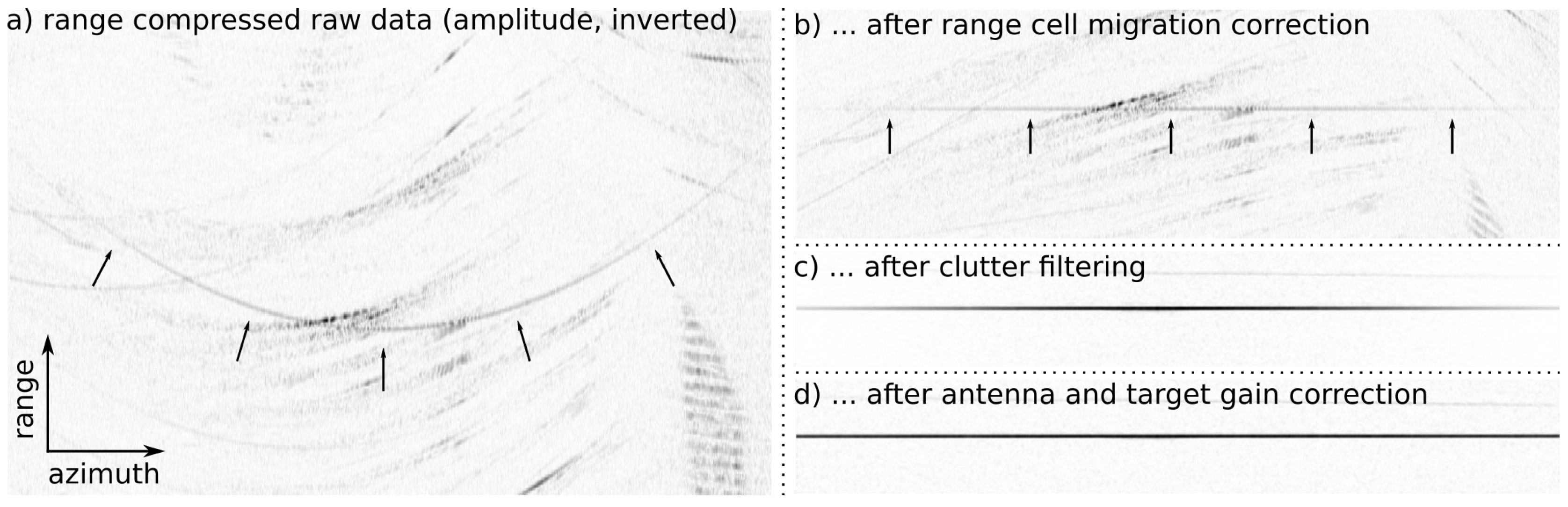
To improve the signal to clutter ratio in the target response, analysis also includes an azimuth-adaptive clutter filter. This filter effectively singles out the directions of arrival corresponding to the reference target. The impact of this filtering step is illustrated in the example response of
Figure 3. The approach is based on the observation that, since the target phase history is flattened in (
8), the Doppler frequency of the response is expected to be constant and close to zero. Significant clutter reduction can therefore be accomplished by simply applying a Gaussian bandpass filter in the Doppler frequency domain:
The filter mean
is set to coincide with the peak of the power spectrum of
. The standard deviation
is set to a value that preserves a certain angular resolution
in the filtered response. The angular resolution may be defined relative to the overall angular response width in azimuth
such that
The results shown in this section and elsewhere in the paper are based on an angular resolution .
Finally, accurate radiometric calibration requires an estimate of the clutter energy remaining in the reference target response after filtering. To this end, the average clutter energy per bin is robustly estimated in the azimuth frequency domain. It is defined as the median intensity between two and three kernel standard deviations offset from the peak response:
3.3. Residual Errors
After the expected target response has been accounted for, the analysis result comprises residual errors, i.e., deviations from the expectation, for all combinations of reference target s and data channel : residual intensity variations , residual phase variations and residual range delays .
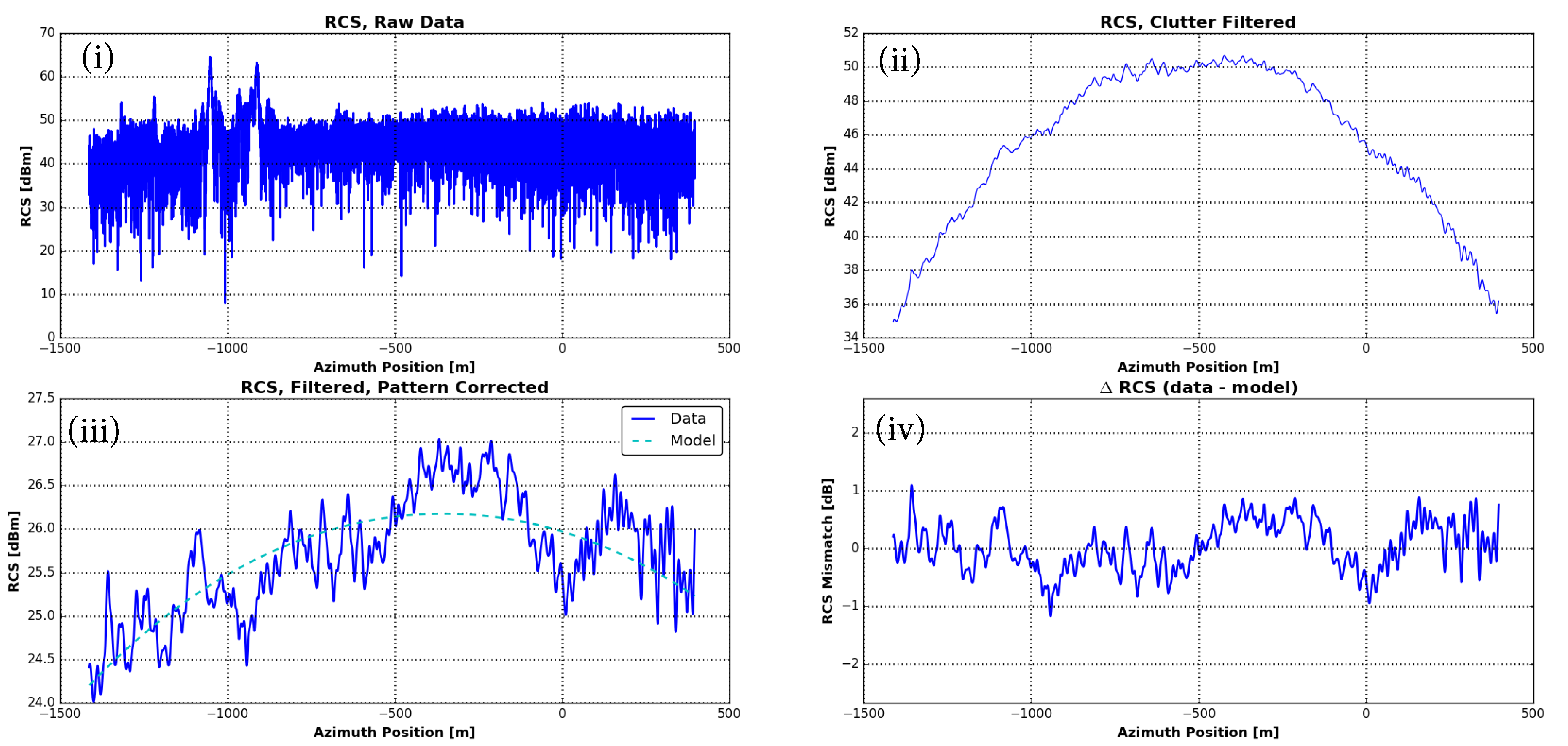
The residual
measures the absolute, unit-less offset, in dB, between the expected and the measured RCS of the reference target. This offset is illustrated in the bottom right plot of
Figure 3. Equation (
8) has accounted for expected systematic intensity variations due to antenna element illumination patterns and the expected target RCS. In addition, the derivation of the absolute RCS offset from the filtered data
of (
10) must also consider the residual clutter intensity of Equation (
13) as follows:
The residual phase , meanwhile, measures phase errors in the target response that can be attributed to target range errors. The sensor position is affected by inaccuracies in the navigation data and the antenna element phase center positions. Similarly, there is a residual uncertainty in the assumed reference target position on ground.
In addition to the phase error above, the target range error can be measured directly. This residual delay is given by the offset of the target peak response away from the expected range. After the range cell migration correction of Equation (
8), the expected peak is in the origin at
, such that he residual delay is estimated as
where
denotes the range sampling frequency of the raw data. The peak response is localized with sub-sample accuracy using the spectral diversity co-registration method described in [
24] using a delta impulse
as a reference signal.
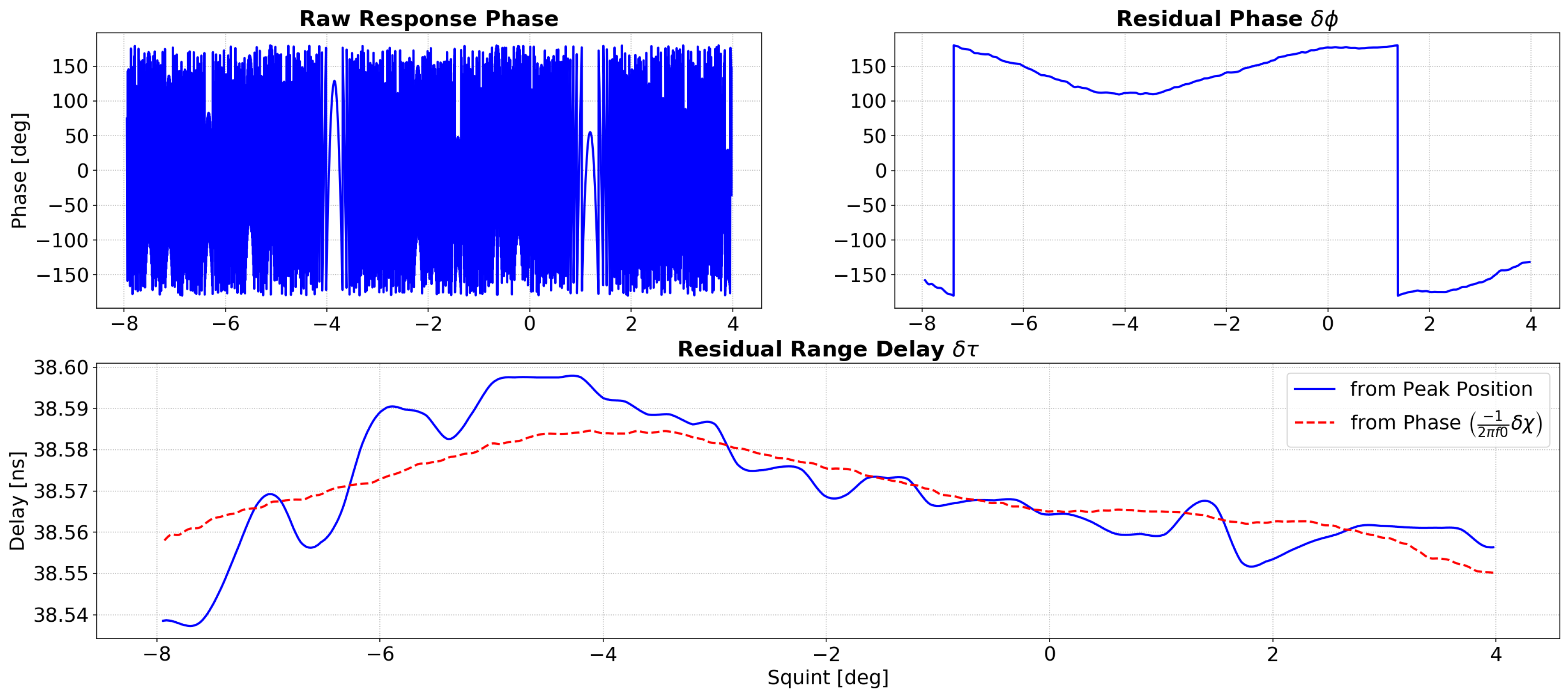
The residual phase of (
15) and the residual delay of (
16) measure essentially the same residual error and, in a certain sense, are complimentary: the phase measurement extremely sensitive but is relative in the sense that it is arbitrarily offset and wrapped in the interval
. The residual delay, on the other hand, is less sensitive but does represent an absolute error. In an attempt to combine the advantages of both measures, the analysis derives the so-called absolute residual phase. It is defined as the offset, unwrapped residual phase:
The absolute phase offset
is set to ensure consistency with the residual delay by enforcing the equality
where
denotes the radar center frequency.
Figure 4 illustrates the information content of the residual phase, the residual delay and the absolute residual phase.
Finally, the calibration approach also uses the so-called target coherence. It quantifies the reliability of the response characterization over azimuth. The coherence is close to one for clean portions of the target response and decreases towards zero where the response is perturbed by residual clutter, system noise or Radio Frequency Interference (RFI). It is denoted
, as it is principally used as a weight when deriving calibration corrections, and is defined as
where ⊗ denotes convolution and
is a low-pass filter that is narrow enough to provide an unbiased coherence estimate. The convolution may, for example, correspond to a moving average window with a size on the order of ∼100 samples.
4. Model-Based Calibration
Calibration proceeds on the basis of residual errors identified in the reference target responses. It entails introducing corrections to sensor parameters that aim to minimize these errors. External calibration thus becomes a rigorous optimization process: explicit models link sensor properties to the expected target response. Appropriate sensor parameter corrections are then the result of error minimization by model inversion.
To make this inversion robust to outliers caused by RFI, system noise and other transient effects, model inversion uses L1-norm error minimization [
25] in favor of least-squares approaches throughout. Given an error functional
that measures some model mismatch over azimuth, L1-norm optimization yields a set of model parameters
that are the solution to
where errors are summed over all target responses in all data channels of all acquisitions.
To ensure that the optimization problem is convex, the following sections uses a closely related objective function
where
is introduced only to ensure numerical stability and is set to
. The convexity of this function guarantees convergence to a global minimum. The minimisation of (
21) is achieved by setting the derivative of the total error with respect to each model parameter
to zero, such that
where
.
While this system of equations is clearly non-linear, it can be solved using a fixed point iteration. In each iteration,
is pre-computed on the basis of the currently available parameter estimates
.
is then treated as a constant in the solution of (
22) and new, refined model parameter estimates are obtained. This process is repeated for a fixed number of iterations (e.g., 10) or until the model parameters have converged.
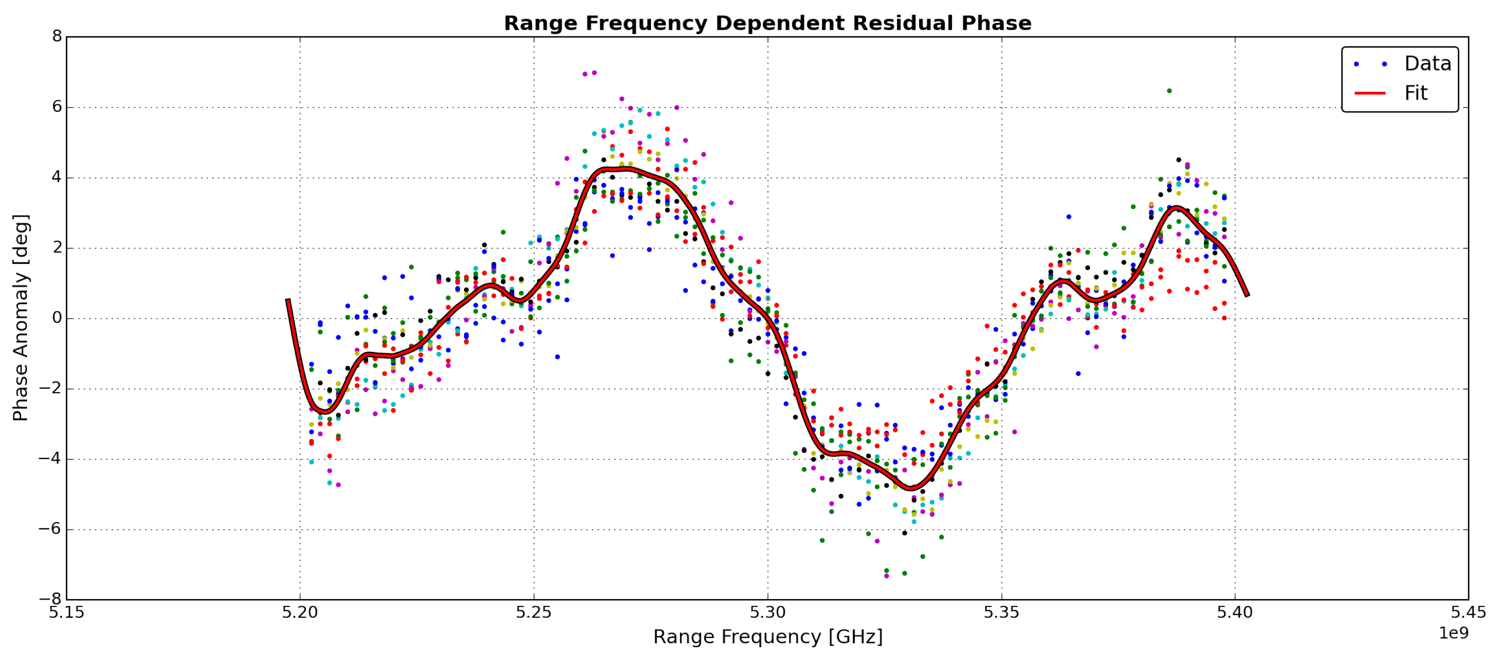
4.1. Range Impulse Response
The aim of the residual range impulse response calibration is to measure systematic, amplitude and non-linear phase variations as illustrated in
Figure 5. Such variations occur within the pulse bandwidth when internal calibration measurements fail to faithfully reproduce the transfer function of the radar instrument.
Estimation begins with pre-processing the filtered raw data to remove constant offsets in gain and residual delay as follows:
The gain and phase of transfer function corrections are estimated independently. Each combination of antenna elements
is thereby associated with corrections
and
that constitute the parameter set
in the corresponding optimization problem (
21). The error measures used are
and
where the coherence
of Equation (
19) is used to emphasize the influence of reliable measurements in the estimated corrections.
The iterative solution of (
22) achieves a robust fit over all pulses in each target response and involves two equations for each discrete range frequency
, one related to
and one related to
. Upon convergence, the complex valued impulse response correction for the antenna element combination
is given by
After residual range frequency response corrections have been obtained, reference target analysis is repeated, as shown in
Figure 1, where these corrections are taken into account in Equation (
9).
4.2. Antenna Mispointing
The aim of the element mispointing estimation is to derive optimal values for the roll/pitch/yaw corrections introduced in Equation (
7). These are the Euler angles underlying the rotation matrix
that transforms instrument to antenna element coordinates in the antenna model of Equation (
6).
The proposed pointing calibration yields attitude angle corrections that minimize variations in the RCS errors
of Equation (
14). The underlying model aims to explain the residual RCS mismatch as a mispointing of individual antenna elements plus a constant gain offset. The corresponding error function takes the form
where
is an unknown constant gain offset characteristic of the channel
, and
denotes the overall, azimuth variant change in the antenna gain, in dB, due to the pointing correction
. The gain change is derived from the two-way complex antenna gain
of Equation (
6) as follows:
where the summations over
are over the radar signal bandwidth and
denotes the nominal complex antenna gain obtained when all pointing correction angles are left at zero.
The minimization of errors of the form (
27) is complicated by the non-linearity of Equation (
28) with respect to the unknown attitude corrections
. The non-linearity is circumvented by linearizing the error function (
27) to obtain
in which
denote unknown incremental refinements to the current mispointing estimate
, and
contains the corresponding, azimuth variant derivatives of
with respect to the three angular axes. These derivatives are obtained numerically from the change in
when the current estimate
is perturbed in each dimension.
The system of Equation (
22) used for minimization comprises three equations for each antenna element
e, with one equation for each angular axis. In addition, it includes one equation corresponding to the constant unknown gain offset in each channel
. After each step of the fixed point iteration, the corrections
are applied additively to the current
estimate and the values of
and the numerical gradients
are updated accordingly. As indicated in
Figure 1, target analysis is repeated to take into account the estimated pointing corrections in (
6).
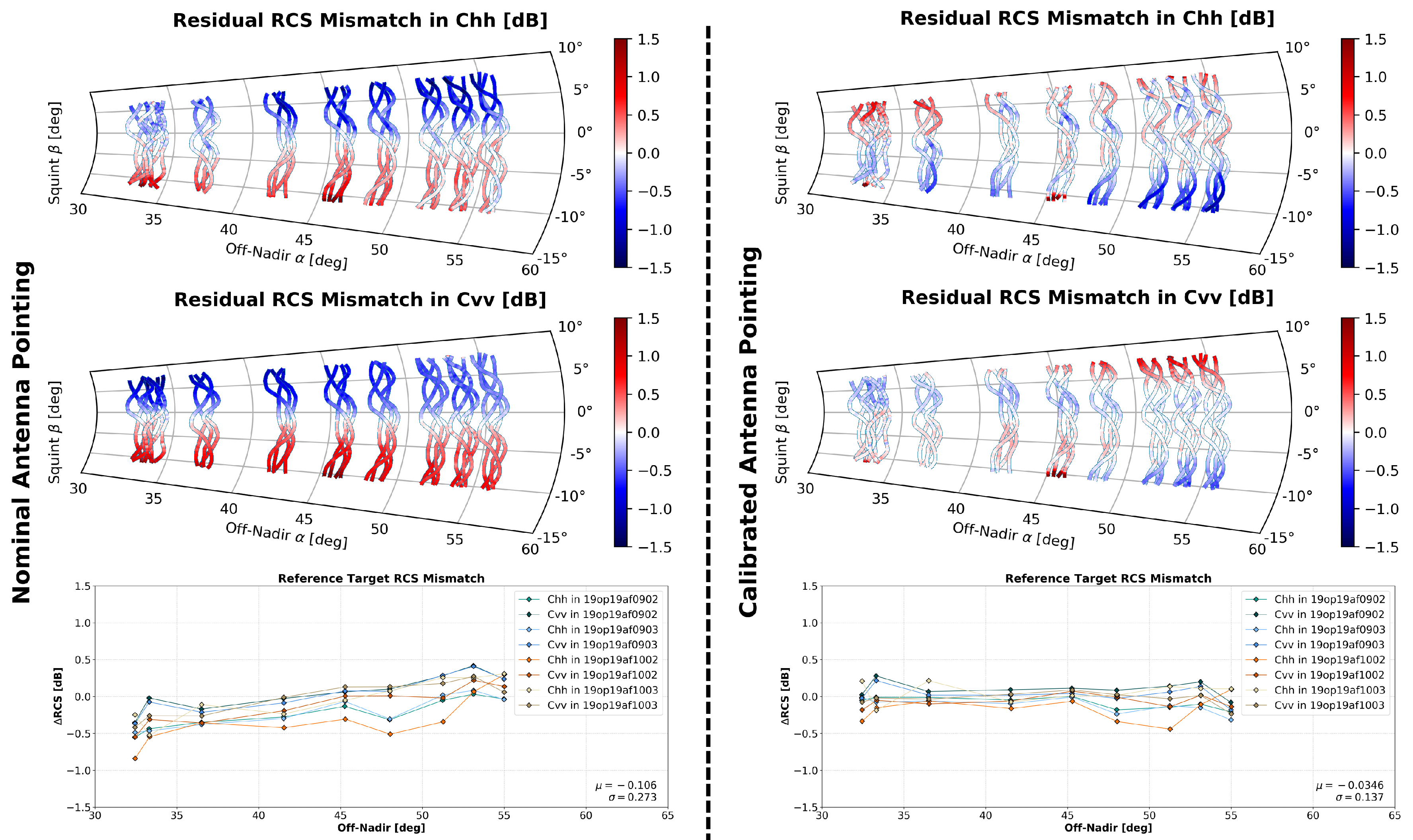
Figure 6 illustrates this optimization process. It shows how a pointing estimate minimizes the mismatch between the expected and the measured reference target RCS.
4.3. Phase Center Positions and Troposphere
Phase center calibration aims to improve the accuracy of the assumed absolute antenna element phase center positions, as parameterized by the vector
introduced in the context of (
2). In addition, this calibration step provides an estimate for the residual tropospheric propagation delay
introduced in Equation (
5). The latter allows corrections to phase center geometry to be clearly separated from other effects. In practice, it may be used to discover any systematic error in the assumed value of
c or, when estimated corrections are unreasonably large or highly variable, instabilities in the assumed radar center frequency. It should be noted that, while this approach is sufficient in airborne SAR applications, it would have to be extended to consider ionospheric effects in low frequency/large wavelength space borne scenarios [
26].
The underlying model relates phase center corrections
and the tropospheric propagation correction
to the observed absolute residual phase of Equation (
17). The corresponding error function to be minimized is given by
where
,
is a constant range offset that is related to residual propagation delays within the sensor, and
is the range offset corresponding to position corrections
projected onto the line of sight vectors
defined in (
3).
While the error measure (
30) aims to introduce corrections that minimize the absolute phase mismatch, it fails to capture an important property of multi-channel SAR: after calibration, any residual errors must be identical in all of the data channels comprising a single acquisition. All channels are equally affected by inaccuracies in the assumed sensor or target positions. To capture this prior knowledge, phase center calibration introduces a second, additional error measure
that penalizes any difference in the residual mismatch between two simultaneously acquired channels
and
. The composed mapping
serves to co-register the channels
and
using the relation between azimuth index and continuous time introduced in the context of (
2).
To accommodate the additional differential error (
32) as well as the coherence weight
of (
19), the fixed point iteration of (
22) is modified to include a second summation over simultaneously acquired pairs of channels
:
where
Generalizing the pattern of (
22), each iteration involves pre-computing two
terms, one for each error measure. The parameter set
comprises the tropospheric propagation correction
, the corrections
for all antenna elements
e as well as channel dependent, constant range offsets
.
4.4. Interferometric Baselines
The calibration procedure described in the preceding section yields refined estimates of the absolute antenna element phase centers. These estimates are sufficient to provide consistently high geometric accuracy in the focused SAR imagery. They are still less accurate, however, than the limit set by residual errors in the assumed sensor and reference target positions. This residual inaccuracy is on the order of a few centimetres for position information derived from differential Global Positioning System (GPS) measurements. As such, it is still far too large for interferometric applications. In interferometry, phase differences, rather than absolute positions, are of central importance.
This section introduces a calibration procedure that precisely determines interferometric baselines, i.e., the spatial separation of antenna element phase centers, to ensure phase consistency among all the channels of a multi-channel SAR sensor. Baseline calibration, as illustrated in
Figure 7, is based on the residual interferometric phase between two simultaneously acquired data channels
and
. It is obtained as
where
denotes the residual phase of (
15) and
is used to achive the co-registration of the channels
and
in time, as in (
32). For a given channel combination
, this results in a set of phase vectors
corresponding to all available reference targets
s = 1, 2, ⋯. To be of use in 3D baseline refinement, these phase differences must be made consistent by unwrapping them. To this end, each phase measurement
is associated with a 2D coordinate
that parameterizes the azimuth variant angular propagation direction towards the target as in Equation (
6). Once the interferometric phase measurements comprising a set such as that of (
36) have been thus embedded in the 2D angular domain, a phase unwrapping algorithm for sparse grids (In view of phase offset calibration, described in
Section 4.5, the unwrapping process should only add or subtract multiples of
and not introduce arbitrary phase offsets.), for example [
27] or [
28], is applied to obtain unwrapped phase vectors
The error model functional
used for baseline refinement aims to minimize residual interferometric phase errors
by introducing antenna element phase center position adjustments
, which are incremental refinements of the corrections
introduced in the previous section.
where
denotes the azimuth variant, cumulative change in line of sight distance to the reference target
s due to lever arm corrections
with
. The variable
absorbs arbitrary constant phase offsets specific to the channel combination under consideration, while the differential coherence weight
is defined in (
34).
As in the case of (
33), the fixed point iteration of (
22) must be modified to accommodate the summation over pairs of channels
. In addition, interferometric baseline calibration deals only in channel differences and is ill-posed unless the optimization is further constrained. To this end, the optimization includes an additional penalty for displacements of the geometric centre of the antenna array:
The fixed point iteration for baseline calibration, including the constraint above, therefore uses a system of equations
where the set of model parameters
comprises phase center position refinements
and constant phase offsets
. Note that the tropospheric propagation correction
retains the value estimated previously and is treated as a known constant during baseline calibration. After the fixed point iteration has converged, the refinements
are added to the previously obtained phase center position corrections
.
4.5. Calibration Constants
The procedures described in the preceding sections have provided range frequency and propagation direction dependent corrections. The last step in the external calibration is then to introduce calibration constants. These account for systematic offsets in gain, delay and phase that are inherent to the sensor and are not related to the physical characteristics of the imaged scene.
Indeed, such constants have already been estimated: gain offsets
, range offsets
and phase offsets
are byproducts of the minimization of error measures (
29), (
30) and (
39), respectively. As corrections are introduced sequentially, however, gain and delay offsets need to be re-estimated to ensure consistency. Robust re-estimation is accomplished by solving minimization problems of the form (
21) for simplified versions of the error measures (
29) and (
30). Simplification entails symbolically substituting
and
, such that the model parameter sets
are reduced to the calibration constants of interest.
While the calibration constants and can be easily and conveniently applied to the raw data of each channel before SAR focusing, the phase calibration constants would have to be applied each time an interferogram is formed. In practice, it is therefore desirable to derive phase calibration information for individual channels, such that
Solving this system of equations is not straight-forward due the fact that the interferometric phase is wrapped. Constants for individual channels can, however, be obtained by constructing a graph with nodes
connected by directed edges associated with phase differences
. A phase unwrapping algorithm for arbitrary grids, such as [
27,
28], can then be used to obtain the desired individual channel calibration constants.
5. Results and Discussion
The calibration approach described in previous sections is part of the operational processing environment for DLR’s multi-channel, airborne F-SAR [
8] and DBFSAR [
29] instruments. The external calibration of these sensors is an ongoing activity that is carried out several times each year to account for upgrades to the sensor hardware, the fact that the radar hardware as well as the antenna mounts need to be re-installed after the research aircraft has been engaged in other scientific activities and, last but not least, to regularly monitor the system stability throughout periods of scientific SAR data acquisition campaigns.
The external calibration of these sensors involves dedicated calibration data acquisitions over a calibration field that is permanently installed at the Kaufbeuren airfield in southern Germany. This installation comprises 9 trihedral radar reflectors ranging in leg-length from m to m, as well as a single dihedral reflector rotated by 22.5 in the line of sight to produce equally strong returns in the co- and cross-polarizations. The trihedral reflectors are deployed across the sensor swath at roughly equal intervals corresponding to off-nadir angles in the range to .
The results presented in the following sub-sections are, unless otherwise noted, based on SAR data acquired as part of the 2019 F-SAR calibration campaign
OP19AF with 10 independent flights from February to June. Each flight comprises roughly 15 SAR acquisitions, in each of which several of the frequency bands X, C, S and L are acquired simultaneously. Almost all of the data acquired are fully polarimetric and some feature polarimetric single-pass interferometry at X- or S-band. The illustrations in
Section 3.2 and
Section 4 are also derived from the raw data collected in this calibration campaign.
Each of the following four sub-sections highlights a particular type of calibration correction. The results presented aim to show how each correction improves the fidelity of SAR measurements. In addition, the results illustrate the types of errors that can be corrected using the approaches developed. Furthermore, the experimental results show that the analyses carried out on range compressed raw data transfer to the focused SAR imagery. They also aim to show that such improvements represent external calibration. The corrections are seen to address systematic errors, rather than merely correcting for transient effects. This is accomplished by showing that results are consistent over multiple independent calibration data acquisitions. In other experiments, calibration corrections are seen to improve the quality of information derived from raw data acquired in the course of scientific measurement campaigns.
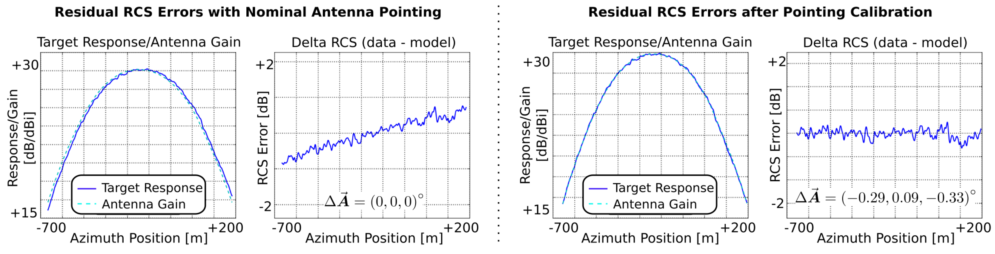
5.1. Radiometry
Other than the comparatively trivial constant gain offset of
Section 4.5, the calibration process affects the radiometric accuracy of the processed SAR data through the pointing estimate
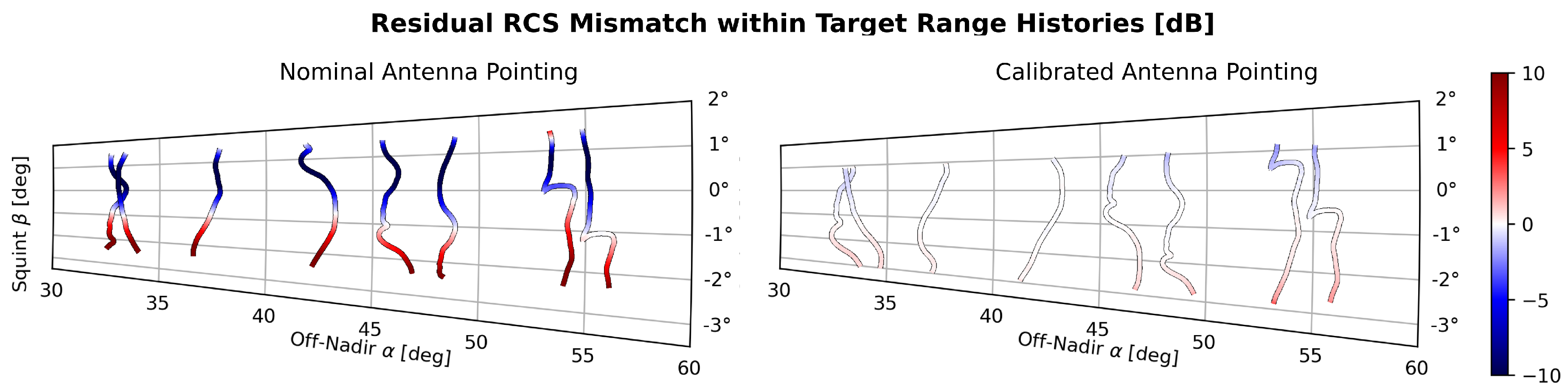
. The impact of the antenna pointing correction is illustrated by the C-band examples of
Figure 8 (One of the many responses shown in this Figure was also used as a basis for
Figure 6 above.) In the polar plots of the first two rows, each reflector response is represented as a line in a coordinate system similar to (
37): azimuth indices are mapped to a propagation direction. This direction is parameterized by squint and off-nadir angles in the antenna reference frame. The trajectories are non-linear and differ from acquisition to acquisition due to variations in the platform attitude angles. The plots in the third row, meanwhile, are based on the analysis of reference targets in focused SAR imagery. In these plots, each reference target is represented by a single data point. Lines connect all targets imaged within a single channel.
The polar plots in the left column clearly show a systematic RCS variation of ±1.5 dB along azimuth, which is largely compensated for by the pointing correction introduced. By contrast, the evaluation in the third row is based on focused SAR data after azimuth compression. As such, it is therefore insensitive to large, systematic variations along the range history of targets. In this light, the estimated standard deviation of 0.3 dB in the bottom left plot is seen to be a gross misrepresentation. Instead, errors on the order of 1 dB are to be expected as the squint angle varies. Such variation is to be expected when data are acquired under different conditions in the field.
The plots in the right column show that the pointing estimate effectively reduces the systematic errors along azimuth. Indeed, it even reduces the RCS mismatch measured in the focused SAR data, as shown in the last row. The polar plots also show, however, that residual RCS errors, which cannot be attributed to antenna pointing, remain. The residual errors and their visualization are helpful in characterizing these types of errors and identifying potential causes. In this case, residual errors are possibly linked to an issue with the antenna pattern measurement.
Figure 9 illustrates the impact on antenna pointing calibration for data acquired by the DBFSAR sensor. The acquisitions were carried out over the Kaufbeuren calibration site during the
DATLAS test flights of 2018. The results pertain to one of the channels of the six-phase center ATI/GMTI configuration of DBFSAR. They were acquired at X-band in VV polarization and with a bandwidth of 800 MHz. The sensor, in this particular configuration, uses a single transmit antenna with a narrow beam of
and six separate, wider receive antennas. The pointing calibration yields separate corrections for the transmit and receive antennas. As the Figure caption indicates, the transmit pointing correction is significant: it is comparable to the antenna beam width. The large correction is consistent with the large initial RCS mismatch observed. It is most likely due to a misalignment of the antenna during the on-ground measurement of the antenna pattern.
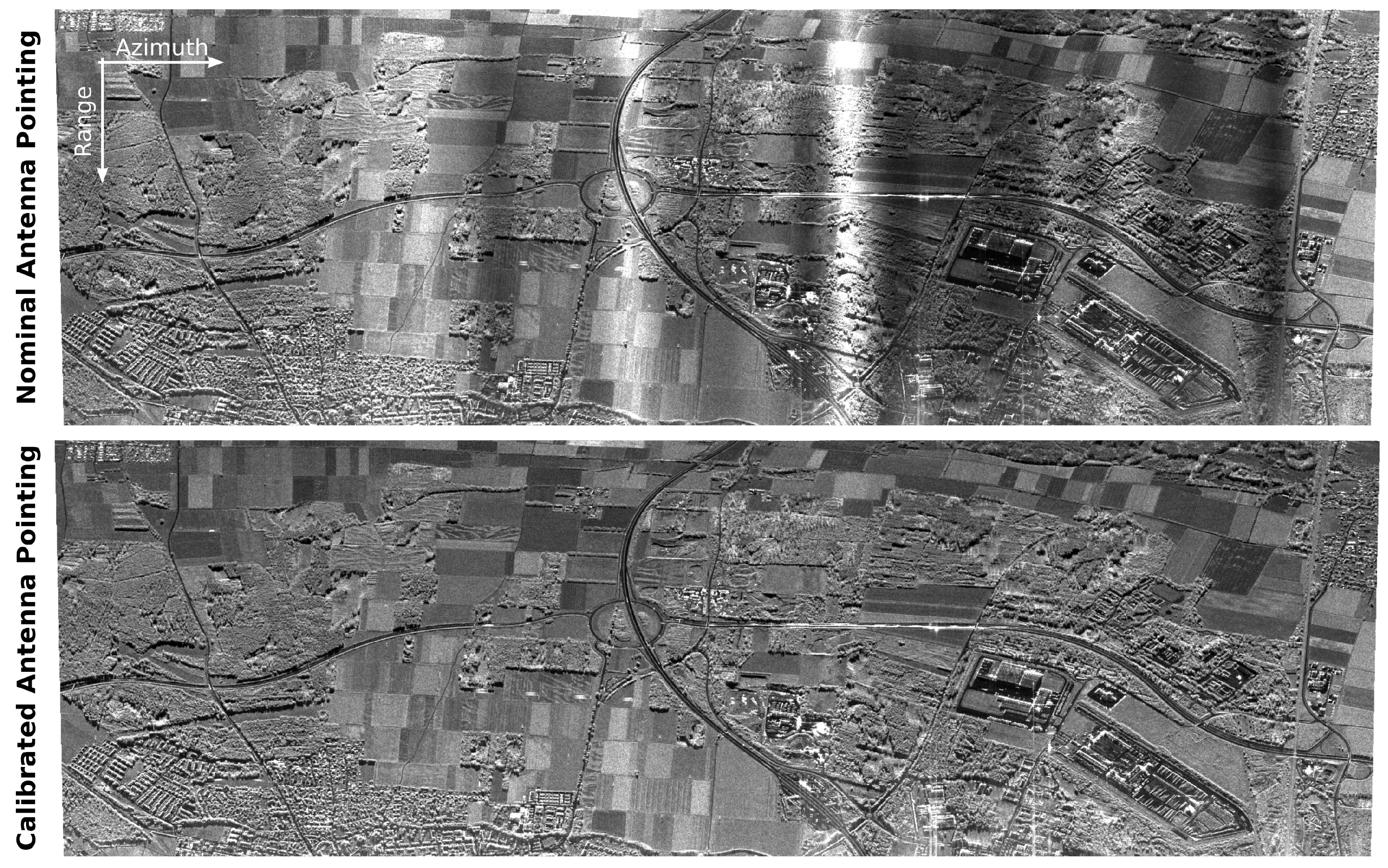
Figure 10 shows the impact of this pointing estimate on focused imagery. These acquisitions took place over the city of Landsberg am Lech, Germany. Although there are no reference targets available for this site, the calibration quality is clearly improved when the estimated pointing correction is taken into account during the antenna pattern correction in SAR processing.
5.2. SAR Impulse Response Function
The proposed calibration approach also has an impact on the impulse response function achieved during SAR processing.
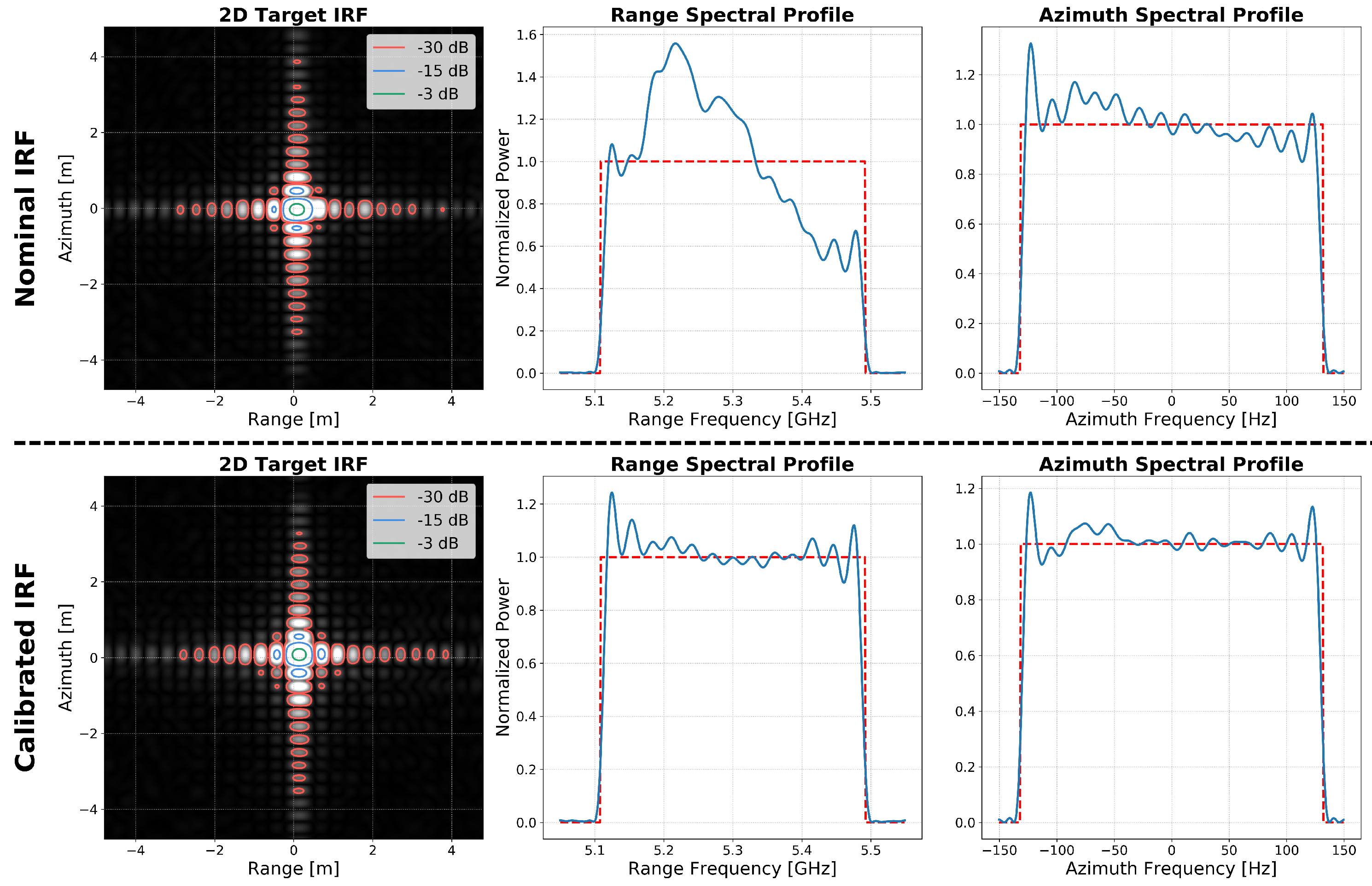
Figure 11 illustrates the improvement achieved for a reference target imaged at C-band: the principal improvement lies in the flattening of the range spectral profile, shown in the middle column, which is due to the response correction introduced in
Section 4.1. A further, but less significant improvement is due to the flattening of the azimuth spectral profile, shown on the right, which is due to the C-band antenna pointing correction that is illustrated in more detail in
Figure 6 and
Figure 9.
5.3. Geometric Accuracy
Section 4.3 and
Section 4.4 introduce corrections to the assumed multi-aperture antenna array geometry. While the baseline corrections of
Section 4.4 establish inter-channel phase consistency and are generally small, the phase center positions refinements
and tropospheric propagation correction
of
Section 4.3 are potentially large and can have a measurable impact on the geometric accuracy of the focused SAR imagery.
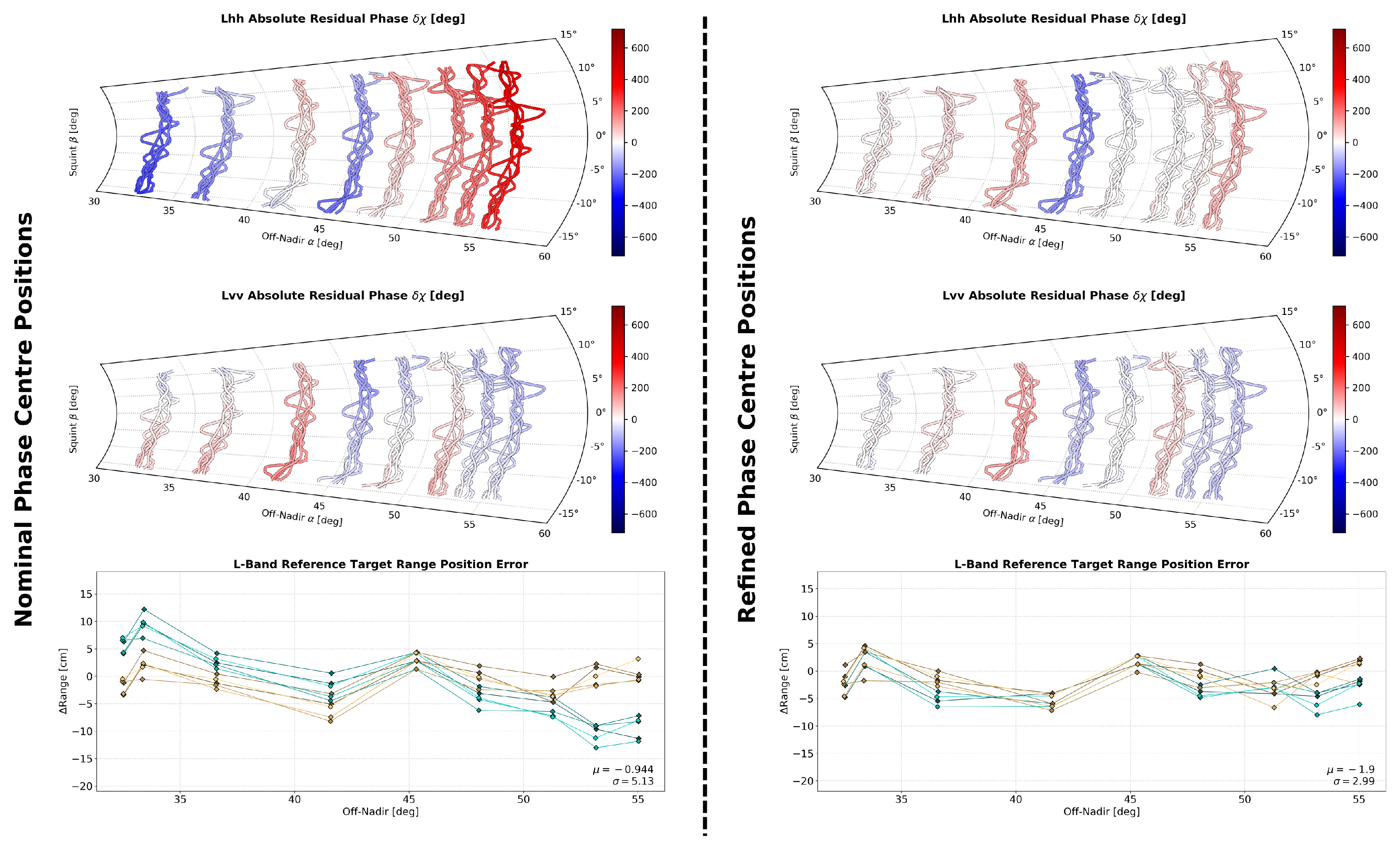
Figure 12 illustrates the impact of antenna phase center calibration on a set of five independent polarimetric L-band acquisitions. The polar plots in the first two rows visualize absolute residual phase errors
within the range histories of trihedral reflectors in the two co-polar channels. As implied by (
18) and illustrated in
Figure 4, these phase errors are directly related to residual range delay or, equivalently, range position mismatch.
The top-left plot suggests that the measured range of reference targets in the HH channel is systematically biased: residual errors clearly show a trend across the sensor swath. This trend is confirmed by the corresponding target range position mismatch measured in focused SAR imagery, as illustrated by the turquoise lines in the bottom-left plot. A comparison of these results with those on the right side of the Figure shows that the estimated phase center position corrections
effectively compensate for this trend. Not only does the correction make the measured target range positions more accurate, but the geometry of the two co-polarized channels has become highly consistent. This is the intended effect of the differential error term (
32). The residual errors measured in focused SAR imagery after calibration, as shown in the bottom-right plot, are largely consistent with the uncertainties to be expected in the sensor navigation data and in the reference target phase center positions obtained via Differential GPS (DGPS).
While
Figure 4 primarily shows the target range mismatch as a function of the off-nadir angle, range error variations do also occur as a function of squint. The top row of plots in
Figure 13 emphasize such variations by showing the residual
after the mean value has been subtracted from each individual range history. The bottom row of plots, meanwhile, show the target azimuth position mismatch. The information in these plots is closely related: a linear phase error along the range history shifts the response in the focused image. As in the range dimension, phase center position calibration improves the overall geometric accuracy in azimuth. Simultaneously, it ensures consistent results across all polarization channels.
The results presented in this section indicate that the proposed phase center calibration model is able to improve the geometric fidelity of focused SAR imagery. It is not, however, possible to quantitatively evaluate the accuracy of the actual position estimates derived as the true phase center positions are simply not known. Qualitatively, however, the results appear plausible. The refined phase centers lie within one or two wavelengths distance from the geometric center of the physical antenna apertures. This holds true for all sixteen phase centers of the F-SAR antenna mount. To further confirm the robustness of the estimate, the L-band calibration detailed in this section was repeated several times. In each iteration, the initial phase center positions were randomly perturbed by m in each dimension and the estimation process was repeated. The resulting phase center estimates were found to be in agreement with a standard deviation of under 2 mm.
A quantitative evaluation is even more difficult for the tropospheric propagation correction
, where optimization yields a value of
for the L-band results of this section. This correction changes the refractivity
from 283, the assumed default value, to 342 parts per million. Both of these values are plausible, in that they are reproducible by stablished models for reasonable choices of temperature, pressure and relative humidity [
30]. While there has not been a systematic effort to validate this aspect of the calibration model further, phase center position corrections are generally smaller and appear more plausible when the tropospheric propagation correction is included in the underlying model. A rigorous analysis of this calibration parameter is, however, beyond the scope of the present discussion. To do so would require additional ground truth and simulations.
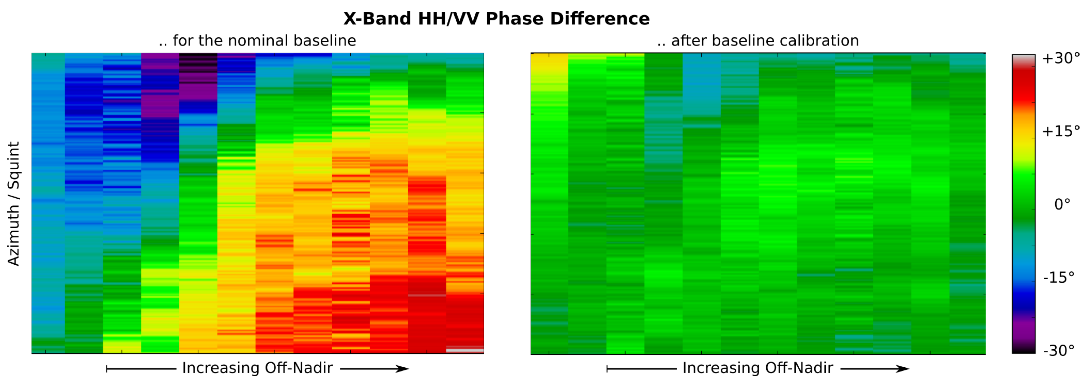
5.4. Single-Pass Interferometry and Polarimetry
Interferometric and polarimetric applications, as well as DBF imaging, rely on phase consistency among data in several channels simultaneously acquired by the SAR sensor. This section presents results that illustrate how propagation direction independent phase consistency is achieved by the baseline calibration approach described in
Section 4.4. The results in this section pertain to data acquired with the X-band polarimetric across track interferometer of F-SAR in 2014.
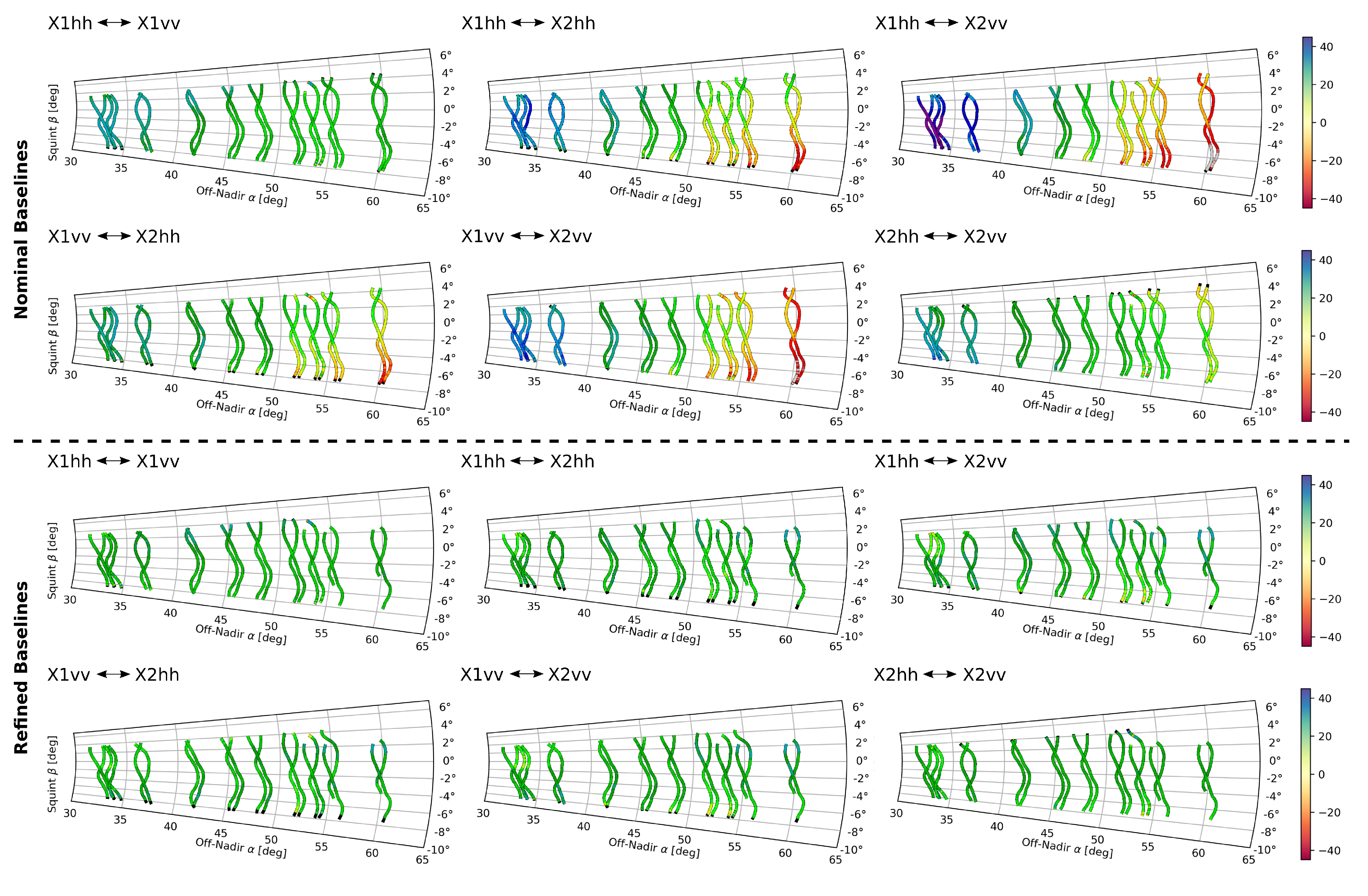
The impact of the baseline calibration process on the inter-channel phase differences of the interferometer is illustrated in
Figure 14. The polar plots show phase differences between the range histories of reference targets deployed in the calibration site. The underlying raw data was acquired during the calibration campaign
OP14AF. The evaluation covers all unique interferometric pairs among the co-polar channels acquired simultaneously by the interferometer. These are four channels corresponding to the two antennas, X1 and X2. The top and the bottom halves of the figure juxtapose interferometric phase errors before and after baseline calibration. The results clearly show that systematic trends are effectively removed from the two independent interferometric calibration data acquisitions considered. The evaluation shows that the errors addressed are, indeed, systematic across independent acquisitions and that the proposed baseline correction model is able to simultaneously explain residual errors in all possible channel combinations of a multi-channel SAR acquisition.
Table 1 lists the position refinements corresponding to the results of
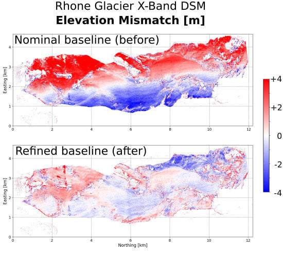
Figure 14. Baseline calibration shifts the phase centers of the interferometer on the order of 1 mm. To further validate this correction,
Figure 15 summarizes results obtained during the scientific measurement campaign
ICESAR, which included acquisitions over the Rhone Glacier in Switzerland that were carried out days after the calibration acquisitions of
OP14AF in September 2014. The results show how the baseline corrections of
Table 1 significantly improve the consistency of digital surface models (DSMs) derived from F-SAR acquisitions with opposing look directions. The original DSM difference shown in the bottom left of
Figure 15 is dominated by a clear trend. The result after calibration, on the other hand, appears to be free of systematic errors. Instead, it shows differences that may be of scientific interest: they could be related to variations in the penetration depth of the radar signal that depend on the local incidence angle.
5.5. Calibration of Under-Sampled SAR Data
As the proposed calibration technique does not require azimuth compression, it does not require the azimuth sampling to fulfill the Nyquist criterion. As argued in
Section 2, the latter point is of practical relevance in the context of DBF techniques, where independent channels are under-sampled but need to be interferometrically calibrated. Relevant examples of future spaceborne systems include HRWS systems with multiple azimuth apertures [
31,
32] but also multiple beam systems operating the SCORE concept to cover a larger swath [
19].
Figure 16 illustrates, qualitatively, why sub-sampling is not an issue in the proposed approach. It compares the results of target analysis obtained for a single target at the full channel Pulse Repetition Frequency (PRF) and after the sampling rate has been artificially reduced by dropping two out of every three pulses of raw data. While the phase and frequency content of the raw data are, of course, severely affected by the sub-sampling, the inputs to the actual calibration process (the residual errors shown in the bottom two rows) remain largely unaffected due to the compensation of the model phase (
5) in the response correction of (
8).
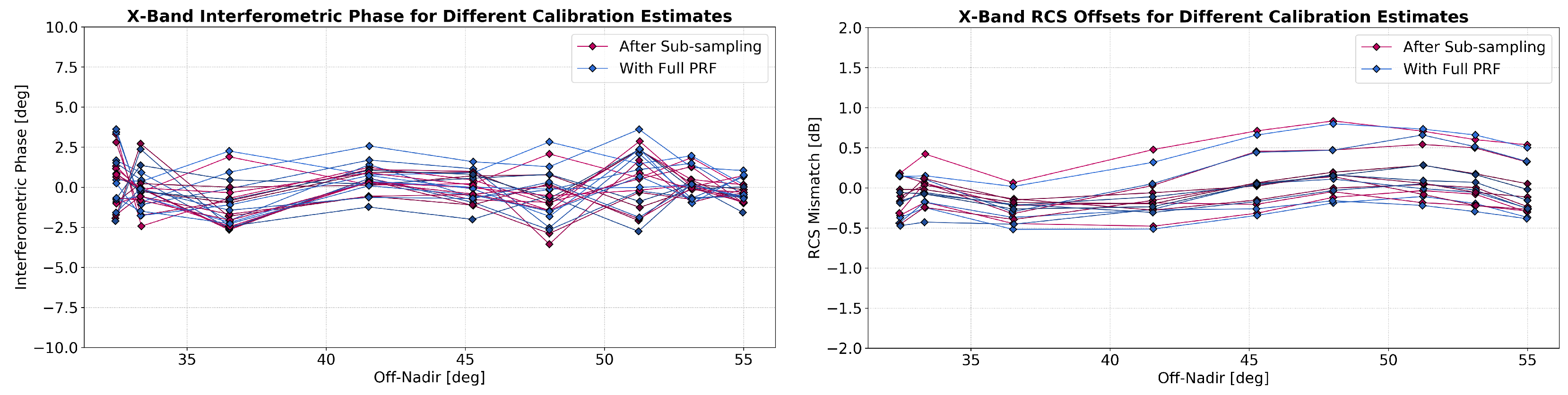
Table 2 quantifies the impact of sub-sampling on the calibration of the four X-band phase centers of the F-SAR across track interferometer. To derive these results, the sub-sampling of
Figure 16 is applied to all raw data channels. The first three columns show the difference in the absolute phase center position. These differences amount to an offset of around 1 cm that has no measurable impact on the geometric accuracy of the data: constant range delays are absorbed by calibration constants, while the variation across the swath is negligible. The relative position changes, obtained by subtracting the mean from each of the first three columns. These are given in the middle columns and are on the order of 1 mm. The pointing changes, given in the last three columns, are significantly smaller than
. As illustrated in
Figure 17, these baseline and pointing changes do not have a measurable impact on the observable calibration quality.
5.6. Limits of Applicability
This section briefly discusses the limits of the estimation algorithms presented in preceding sections. These limits are defined in terms of the magnitude of errors that can be corrected. They are summarized in
Table 3.
The maximum antenna pointing correction
is roughly equal to the antenna beam width. It therefore depends on the frequency band and the antenna design. The results presented in
Section 5.1, and
Figure 10 in particular, demonstrate that the approach can correct for mispointing of a magnitude comparable to the azimuth beam width. This result, however, is close to the limit of what is possible for several reasons. Firstly, the linear approximation of Equation (
29) eventually fails: assuming, for simplicity, that the antenna gain in the main beam is roughly quadratic, the 1 st order Taylor expansion implied in the approximation of (
27) by (
29) is only valid within the main beam (where the difference of two approximately quadratic functions is approximately linear). When this linear approximation fails, the fixed-point iteration for the pointing estimate will converge to meaningless results or may even diverge entirely. Secondly, very large pointing errors would make it difficult to even localize the reference target response in the raw data. Additional pre-processing steps might be required to bootstrap the calibration process.
In the case of the maximum phase center position correction
, simulations with artificially displaced phase centers suggest that errors of at least 10 m can be corrected: for the X-band data of
Section 5.5, the corrected positions agree to within margins similar to those reported in
Table 2. Even larger errors were not considered, as they appear of little practical relevance. Eventually, however, the calibration process would fail as the target response lies outside the range interval considered during analysis. Furthermore, these results are also the basis for the limit given for the tropospheric propagation correction
. The maximum correction given in the table, in parts per million, corresponds to a error in the range vector of
m for a typical altitude above ground of 5 km. This limit is far outside the range of variation encountered in nature [
30].
Finally, another limiting factor to be considered in practice is the signal to noise ratio (SNR). The impact of noise may be an issue, as the proposed approach does not involve azimuth compression and therefore does not benefit from azimuth compression gain. The results of
Section 5.5 are relevant in this regard: while they demonstrate that azimuth under-sampling does not present any fundamental difficulty in the calibration approach, under-sampling does ultimately have a detrimental impact on the accuracy attainable. Increasing under-sampling leads to increased clutter levels, even after clutter filtering, as more clutter contributions become aliased with the reference target response. This increase in clutter noise is evident in the plots of
in the last row of
Figure 16. The SNR is clearly not an issue for the sensor and acquisition geometries considered in the preceding sections. Should low SNR be a practical concern, however, the proposed calibration technique may yet remain applicable if either the PRF or the strength of the reference target radar return can be increased.
6. Conclusions
The paper introduces a new approach to the external calibration of multi-channel SAR sensors. A survey of results based on the analysis of multi-channel SAR data acquired by DLR’s airborne F-SAR and DBFSAR sensors suggest that the approach can be used to effectively estimate calibration corrections to counteract propagation direction dependent effects, thereby significantly improving the radiometric and interferometric data calibration quality.
The calibration approach yields antenna phase center position and interferometric baseline corrections in three dimensions as well as three dimensional antenna pointing estimates. The results reported show that the antenna phase center refinement leads to improved and more consistent geometric accuracy in focused SAR imagery and also improves the fidelity of interferometric and polarimetric SAR phase measurements. The antenna pointing estimates, which are provided separately for transmit and receive where the multi-channel scenario demands it, are seen to improve the radiometric accuracy. Pointing corrections also compensate for systematic, residual amplitude variations in the Doppler spectrum after SAR processing.
Unlike current state of the art techniques, the method is based entirely on the analysis of range compressed raw data and does not require azimuth compression. It remains applicable in cases where azimuth compression presupposes accurate calibration and, in particular, can be applied to data that is irregularly or under-sampled in azimuth. This is especially relevant in view of the digital beam-forming techniques envisaged for future HRWS missions, such as the Tandem-L formation [
33].
7. Patents
European Patent Number EP000003364212A1 (”A method and an apparatus for computer-assisted processing of SAR raw data”), published on 22 August 2018.


