Modeling Spatio-Temporal Land Transformation and Its Associated Impacts on land Surface Temperature (LST)

Abstract

Land use land cover (LULC) of city regions is strongly affected by urbanization and affects the thermal environment of urban centers by influencing the surface temperature of core city areas and their surroundings. These issues are addressed in the current study, which focuses on two provincial capitals in Pakistan, i.e., Lahore and Peshawar. Using Landsat data, LULC is determined with the aim to (a) examine the spatio-temporal changes in LULC over a period of 20 years from 1998 to 2018 using a CA-Markov model, (b) predict the future scenarios of LULC changes for the years 2023 and 2028, and (c) study the evolution of different LULC categories and investigate its impacts on land surface temperature (LST). The results for Peshawar city indicate the significant expansion in vegetation and built-up area replacing barren land. The vegetation cover and urban area of Peshawar have increased by 25.6%, and 16.3% respectively. In contrast, Lahore city urban land has expanded by 11.2% while vegetation cover decreased by (22.6%). These transitions between LULC classes also affect the LST in the study areas. Transformation of vegetation cover and water surface into built-up areas or barren land results in the increase in the LST. In contrast, the transformation of urban areas and barren land into vegetation cover or water results in the decrease in LST. The different LULC evolutions in Lahore and Peshawar clearly indicate their effects on the thermal environment, with an increasing LST trend in Lahore and a decrease in Peshawar. This study provides a baseline reference to urban planners and policymakers for informed decisions.

1. Introduction

The world’s population is growing rapidly [1] and people are moving from rural to urban areas [2], leading to a strong increase in urbanization [3]. The number of people living in the global metropolitan regions is expected to increase by ~80% during the period from 2010 to 2050 [2]. During the past few decades, urbanization in and around metropolitan cities all around the world has significantly reduced the fraction of green vegetation cover layer. Green vegetation cover is essential for the equilibrium between the land surface and atmospheric parameters [4,5]. Two of the most important parameters associated with the urban environment are land use land cover (LULC) and land surface temperature (LST) [6,7]. Variation in different land use categories, especially the transformation of vegetation land to the urban area, can effectively influence the LST [8,9,10]. The surface reflectance and roughness of each LULC category are different, so each LULC category has various contributions to the LST because of its unique qualities in terms of energy radiation and absorption [11,12]. Many regions around the world are facing dramatic changes in LULC [13], associated with rapid urbanization [14,15,16] and with large consequences for, e.g., the increase in urban population demands of metropolitan luxuries and facilities for their living, including the construction of new residential and commercial areas, public utilities and road infrastructure [17,18,19,20]. The combined influences of biological factors and anthropogenic activities play a vital role in the transition of LULC [21,22,23,24,25]. Several natural and anthropogenic elements cause LULC changes [26,27,28,29], such as social, economic, biophysical, and political factors [30,31,32].

Remote sensing (RS) is a powerful and effective tool that can provide abundant, multi-spectral, multi-temporal, and real-time data from which information can be distracted which is valuable for monitoring and understanding land development patterns and processes [33]. Satellite remote sensing provides a unique opportunity to monitor the changes in both LULC and LST at high spatial and temporal resolution [7,34,35], which is used in the current study. The launch of the different Landsat satellites since 1972 provides a continuous time series of remote sensing data that are available free of charge for numerous applications in studies on social, economic, and environmental characteristics of urban areas [36]. This long time series can provide a better understanding of the past and recent dynamics in LULC transitions, which can support the development of future policies for urban sustainability [18]. Moreover, the continuous availability of Landsat imagery can also be used to develop and test land use prediction models [37,38]. The utilization of urban growth models [39,40] has reliable and practical capabilities to predict land use land cover change [41,42] and quantify the transition of a LULC class to another one [18], which can help to plan a city while limiting problems due to urbanization [43]. Recent studies showed that for the transition and future predictions of LULC, a CA-Markov Model combined with GIS and remote sensing is an effective and powerful modeling technique [44,45,46,47,48,49,50], which can provide detailed information on a synoptic scale [50,51,52,53,54]. In the CA-Markov model, the cellular automata (CA) detect the spatial location of changes while the Markov chain calculates the future changes [55,56,57]. It has been widely used for the urbanization studies in cities in Wuhan/China [48], HuaHin/Thailand [44], Saga/Japan; SetúbalSesimbra/Portugal [58]; central Germany [56], London/UK [23], Ahmedabad/India [59], Tehran/Iran [55], Santiago/Chile [60] and Foshan/China [61]. Other models have also been used to simulate urbanization processes [62,63,64,65,66,67,68]. However, in this study, the CA-Markov model has been used for reasons provided in Section 2.4, where the CA-Markov model is described in detail.

This study focuses on LULC variations over two urbanized regions in Pakistan, i.e., Lahore and Peshawar. In Pakistan, urbanization has mainly affected the growth of the population in major cities due to a lack of planning and policy. An increase in urban population requires the development of facilities for living, including the construction of new residential and commercial areas, public utilities, and road infrastructure, which ultimately leaves footprints on the environment [62]. Urban growth not only influences socioeconomic change but also causes the loss of farmland [25,63]. In the past several years, the LULC has changed on a large scale in which forest land was transformed into farmland, while farmland has gradually been transformed into urban areas [64]. These transformations have dramatically influenced the environment [65] and often threatens the sustainable urban development [66,67].

In recent years, Lahore, in the province of Punjab (see Figure 1), has experienced massive growth because of the high demand for the urban area. Most of the agriculture and barren land was bought by local developers and the Lahore Development Authority (LDA) and turned into different housing societies and other projects [68,69]. As a result of this urban expansion and over-cutting, the vegetation cover of Lahore has decreased substantially. Moreover, natural land has been replaced mainly by built-up areas, i.e., urbanized areas including buildings, roads, and different other infrastructures [68,69].

Peshawar, in the province of Khyber Pakhtunkhwa (KPK, see Figure 1), has also experienced sudden changes in population growth due to the migration of people from Afghanistan [70]. Following the 1961 census, Peshawar represents 29% of the total population of the province of Khyber Pakhtunkhwa, whereas in 1998 the population in Peshawar had increased to 33% of the entire population of this province [71]. Additionally, in 2013, the provisional government of KPK started the “billion trees project” in the whole region [72], which aims to restore 150 million hectares of the world’s degraded and deforested lands by 2020 (https://en.unesco.org/courier/2019-3/pakistan-green-again/, last access: 20 august 2020), and Pakistan hit its “billion trees” goal in August 2017 (https://www.weforum.org/agenda/2018/07/pakistan-s-billion-tree-tsunami-is-astonishing/, last access: 20 August 2020). Such changes in LULC influence the LST, air temperature, and topography of the neighborhood [73,74]. Therefore, there is a strong need to quantify the individual contribution of different LULC transformations to LST in and around urbanized regions of Pakistan.

In this study, the CA-Markov chain model is applied to simulate the current and future land use dynamics over two metropolitan cities in Pakistan, Lahore and Peshawar. As described above, land use management in these cities was very different, which resulted in contrasting effects on the thermal environment. Overall, this study was conducted to (a) examine the spatio-temporal LULC dynamics for the years 1998, 2003, 2008, 2013, and 2018, (b) predict the LULC in 2023 and 2028 using the Markov and CA-Markov models, and (c) examine the LULC transition into different LULC categories and to quantify its impacts on LST. The results clearly show the effect of different land-use policies on the urban environment and provide direction for reducing environmental problems in future climate scenarios using different choices of LULC. The study area, data collection and models used are described in Section 2, including the motivation for using the CA-Markov model to simulate LULC changes (Section 2.4). The results are presented and discussed in Section 3 and the conclusions from the study are provided in Section 4.

2. Material and Methods

2.1. Study Area

The study area comprises two large cities (Lahore and Peshawar) in Pakistan (Figure 1). Peshawar is the capital of KPK (Khyber Pakhtunkhwa) Province, along the Khyber Pass, near the border of Afghanistan. Peshawar is a magnificent and essential economic, political and military center of the province and Pakistan. Geographically Peshawar is located at 44°15’ N, 71°42’ E and covers an area of 1264 km². According to the census of 2017, a total of 1.97 million people live in Peshawar (http://www.pbs.gov.pk/ last access: 13 July 2020). Lahore is the 2nd largest city in Pakistan and is the capital city of Punjab province. Lahore covers a total area of 1842 km² located between the latitudes of 31°15′–31°43′N and longitudes 74°10′–74°39′E. A total of 11.13 million people live in Lahore according to the statistics of the 2017 census (http://www.pbs.gov.pk/ last access: 13 July 2020).

2.2. Data Collection and Preprocessing

For the analysis of the LULC dynamics and the effect of the LULC transition on the thermal environment in Lahore and Peshawar, satellite imagery including Landsat 5 Thematic Mapper (TM) and Landsat 8 (Operational Land Imager (OLI) was collected (

Table 1. Satellite images used in this study.

Study Region	Row/Path	Year	1998	2003	2008	2013	2018
Lahore	149/036	Date	25 May	31 May	05 June	19 June	01 June
		Sensor	TM	TM	TM	OLI	OLI
Peshawar	151/036 151/037	Date	8 June	13 May	19 June	01 June	30 May
		Sensor	TM	TM	TM	OLI	OLI

). The temporal resolution of the images is 16 days and the spatial resolution is 30 m. All images were freely downloaded from the USGS earth explorer website (http://earthexplorer.usgs.gov/, last access: 4 January 2020). After the preparation of the satellite images vector layer of the administrative boundary of the study area, Lahore and Peshawar were utilized as masks to subset the images for clipping the area of interest (AOI) from the Tagged Image File Format (TIFF). No atmospheric corrections were executed since the Landsat images were cloud-free [75,76]. After this, the thermal bands were used to derive the LST [77,78]. First, the digital number (raw data) of Landsat images thermal bands was converted into radiance and then surface temperature. For LULC maps, visible, near-infrared and shortwave infrared bands of Landsat products were stacked and mosaicked using ARDAS Imagine [79,80]. Supervised classification was used to classify the pixels into four different LULC classes [81]: vegetation, water bodies, built-up, and barren land. After the preparation of LULC maps for each year, the error matrix was constructed to evaluate the accuracy of LULC classes. To this end, ground truth samples for each land-use class were taken from random locations using Google Earth [82] and compared with the collocated LULC pixel. The percentage accuracy of each class was evaluated in ArcGIS using frequency analysis and error matrix [83]. The results are presented in Section 3. The LST retrieval is visualized in the flowchart of Figure 2, with details described below.

2.2.1. Conversion of Raw Landsat Data into Radiance

The Landsat data are downloaded as raw data (digital numbers) which needs to be converted to spectral radiances (Lλ) by using the information in the LANDSAT metadata header file [16]:

$${\mathrm{L}}_{\mathsf{\lambda }} = \frac{{\mathrm{LMAX}}_{\mathsf{\lambda }}-{\mathrm{LMIN}}_{\mathsf{\lambda }}}{\left({\mathrm{Q}}_{\mathrm{calmax} }-{ \mathrm{Q} }_{\mathrm{calmin} }\right)} \times ({\mathrm{Q}}_{\mathrm{cal} }{}_{ }-{ \mathrm{Q} }_{\mathrm{calmin} }) + {\mathrm{LMIN}}_{\mathsf{\lambda }}$$

(1)

where ${\mathrm{L}}_{\mathsf{\lambda }}$ is the spectral radiance (Wm⁻² sr⁻¹µm⁻¹⁾, LMAX_λ is the spectral radiance scaled to Q_Calmax (W m⁻² sr⁻¹ μm⁻¹). LMIN_λ is the spectral radiance scaled to Q_Calmin (W m⁻² sr⁻¹ μm⁻¹). Q_Calmax is the maximum quantized calibrated pixel value (DN = 255) that corresponds to LMAX_λ. The minimum quantized calibrated pixel value (DN = 0) corresponds to LMIN_λ. Q_Cal is the quantized calibrated pixel value (DN) [84,85].

2.2.2. Conversion of Radiance to Reflectance

The radiances calculated using Equation (1) were converted into reflectance using Equation (2) [85]:

$$\mathrm{r}=\frac{\mathsf{\pi }\times {\mathrm{L}}_{\mathsf{\lambda }}\times {\mathrm{r}}^2}{{\mathrm{E}}_{\mathrm{sun}}\times \mathrm{Cos}ø\times \mathrm{dr}}$$

(2)

where r is the planetary reflectance (dimensionless), L_λ is the spectral radiance at the sensor aperture (W m⁻² sr⁻¹ μm⁻¹), dr = 1 + 0.033cos (D × 2 × 3.14)/365), where D is the day of the year, Esun is the mean solar atmospheric irradiance (W m⁻² μm⁻¹), θ is the solar zenith angle (degree), θ = (90 − B), and B is the Sun elevation angle. dr is the inverse square of the earth-sun distance (astronomical unit).

2.3. Land Surface Temperature (LST) Retrieval

For the retrieval of LST, Landsat images were used with a temporal resolution of 16 days and a spatial resolution of 30m. The LST was derived from the Landsat thermal bands using the methodology recommended by [86]. In the first step, the radiance of the thermal band calculated using Equation (1) was converted into brightness temperature (TB) using Equation (3):

$$\mathrm{TB} =\frac{K_2}{ln \left[\left(\frac{K_1}{L_{\lambda }}\right)+1 \right]}$$

(3)

where; K1 and K2 are conversion constants. For Landsat8 OLI, K1 = 774.89 mW cm⁻² sr⁻¹ μm⁻¹ and K2 = 1321.08 K; Landsat5 TM, K1 = 607.76 mW cm⁻² sr⁻¹ μm⁻¹ and K2 = 1260.56 K. In the second step, the land surface temperature was derived using the following relation [87]:

$$\mathrm{LST} = \frac{T_B}{1 +\left(\frac{\lambda T_B}{\rho }\right)\ln ϵ}$$

(4)

where λ (≈ 11.5 µm) is the effective wavelength of the thermal bands. $\mathsf{\rho }$ = $\left(\mathrm{hc}\right)/\mathsf{\sigma }$ = 1.438 × 10⁻² mK, where σ is the Boltzmann constant (1.38 × 10⁻²³ JK⁻¹), $h$ is the Planck constant (6.626 × 10⁻³⁴ Js) and c is the speed of light (3.0 × 10⁸ ms⁻¹), ϵ is the land surface emissivity with values of 0.95, 0.92 and 0.9925 for vegetation, build-up and water surfaces, respectively [88]. Land surface emissivity ($\mathsf{Ɛ}$) was estimated using the NDVI thresholds method as proposed by [77], using the following equations:

$${\mathrm{d}}_{\mathsf{Ɛ}}=\left(1_{-}{\mathsf{Ɛ}}_{\mathrm{s}}\right)\times \left(1-{\mathrm{p}}_{\mathrm{v}}\right)+\mathrm{F}\times {\mathsf{Ɛ}}_{\mathrm{V}}$$

(5)

where ${\mathsf{Ɛ}}_{\mathrm{v}}$ is the vegetation emissivity, Ɛ_s is the soil emissivity, F = 0.55 is the shape factor (Lim et al., 2012), and Pv is the vegetation proportion, which was obtained using Equation (6) [87]:

$${\mathrm{P}}_{\mathrm{v}}={\left(\frac{\mathrm{NDVI}-{ \mathrm{NDVI}}_{\min }}{{\mathrm{NDVI}}_{\max } -{ \mathrm{NDVI}}_{\min }}\right)}^2$$

(6)

where NDVI is derived by using Equation (7) [89]:

$$\mathrm{NDVI}=\frac{\left(\mathrm{NIR}-\mathrm{RED}\right)}{\left(\mathrm{NIR}+\mathrm{RED}\right)}$$

(7)

In Equation (7), NIR and RED are reflectances. For Landsat5 (TM), NIR is the reflectance measured in band 4 at wavelength λ = 0.76–0.90 μm and RED is the reflectance measured in band 3 with λ = 0.63–0.69 μm. In Landsat8 (OLI), NIR is the reflectance measured in band 5 with λ = 0.85–0.87 μm and RED refers to the reflectance measured in band 4 with λ = 0.64–0.67 μm. NIR and RED values were retrieved using Equation (2).

In this study, the focus is the effect of LULC transition on LST, which is stronger in the hottest months in Pakistan, i.e., May, June, and July. Therefore, LST trends over the study period were evaluated using averages over these 3 months.

2.4. Simulation of LULC Changes Using the CA-Markov Model

The CA-Markov model was used for LULC simulations [90] because it provides a powerful technique to study urban growth trends and future predictions [54,91,92,93] and detailed information on a synoptic scale [50,51,52,53,54]. The CA-Markov model can be applied to simulate future LULC distributions. It consists of two parts, the CA model and a Markov chain model. The Markov chain model estimates the state of the LULC change between two time intervals to predict future changes. This model not only describes the conversion states between the land use types but can also account for the transfer rate among different land use categories. It can be used in spatial modeling for forecasting future LULC [94]. The CA model consists of a regular grid of cells, with properties that can change in time according to fixed rules and depend on the current state of a cell and its neighboring cells. Because of these characteristics, it has also been applied for simulating the LULC process [95,96]. In the CA model used here, the specific transition rules apply to 3 × 3 neighboring cells, i.e., a central cell with 8 neighbors which affect the properties of the central cell. For the application of the CA model to simulate the future LULC, the properties of LULC types should be considered, for instance, the built-up area cannot transfer into water in the near future [50]. The Markov model can be mathematically described as Equation (8):

$$\mathrm{S} \left(\mathrm{t}+1\right)=\mathrm{Pij}*\mathrm{S}\left(\mathrm{t}\right)$$

(8)

where S represents the land use status at time t, and S (t + 1) is the land-use status at time t + 1, while Pij is the transition probability matrix in a state which is calculated as Equations (9) and (10) [97]

$$\Vert \mathrm{Pij}\Vert = \Vert \begin{array}{ccc}{\mathrm{P}}_{1,1}& {\mathrm{P}}_{1,2}& {\mathrm{P}}_{1,\mathrm{N}}\\ {\mathrm{P}}_{2,1}& {\mathrm{P}}_{2,2}& {\mathrm{P}}_{2,\mathrm{N}}\\ {\mathrm{P}}_{\mathrm{N},1}& {\mathrm{P}}_{\mathrm{N},2}& {\mathrm{P}}_{\mathrm{N},\mathrm{N}}\end{array}\Vert$$

(9)

$$\left(0\le \mathrm{Pij} \le 1\right)$$

(10)

where P is the transition probability; Pij stands for the probability of converting from current state i to another state j in next time; and PN is the state probability of any time. The Low transition will have a probability near (0) and high transition have probabilities near (1) [97].

2.5. Validation of the LULC Prediction Model

The Kappa Index of Agreement (KIA) approach was used to check the validity of the CA-Markov model. The Kappa statistic measures the accuracy of a classification relative to a completely random classification on a scale from 0 (utterly random assignment of class labels) to 1 (100% accuracy of class label assignment) [98,99]. KIA can be calculated using Equation (11):

$$\mathrm{KIA}=\mathrm{Pr}\left(\mathrm{a}\right)-\mathrm{Pr}\left(\mathrm{e}\right) /1-\mathrm{Pr}\left(\mathrm{e}\right)$$

(11)

where Pr (a) represents the observed agreement, and Pr(e) represents chance agreement. The process is described in more detail in Section 3.2.

2.6. Relationship between LST and LULC:

The relation between LST and LULC was calculated by linear regression, using the linear regression expression in the Curve Fit tool by using ARC GIS; Curve Fit is an extension of the GIS application ArcMap that allows the user to run regression analysis on a series of raster datasets (geo-referenced images) (https://www.umesc.usgs.gov/management/dss/curve_fit.html/, last access: 19 January 2020). Later on, the zonal statistic was applied to get the values. The equation of linear regression is described below:

$$\mathrm{Y}=\mathrm{aX}+\mathrm{b}$$

(12)

where Y is the dependent variable, X is the independent variable, b is the slope of the line and a is the y-intercept.

3. Results

3.1. Land Use Land Cover (LULC) Dynamics

Maps of the LULC in Lahore and Peshawar, for one selected day in each of the years 1998, 2003, 2008, 2013 and 2018 (Table 1), were obtained after preprocessing and supervised classification. The results are presented in Figure 3. The accuracy of the LULC classification was assessed using ground truth data obtained from Google Earth and the results are presented in

Table 2. Accuracy assessment of land use classification in Lahore and Peshawar (%).

Study Region	LULC Classes	1998	2003	2008	2013	2018
Lahore	Water	0.80	0.78	0.82	0.80	0.77
	Vegetation	0.72	0.76	0.73	0.79	0.80
	Built-up	0.83	0.79	0.80	0.78	0.77
	Barren Land	0.79	0.70	0.78	0.77	0.70
	Overall Accuracy (%)	0.78	0.76	0.78	0.79	0.76
Peshawar	Water	0.77	0.80	0.74	0.77	0.71
	Vegetation	0.80	0.72	0.70	0.70	0.75
	Built-up	0.71	0.83	0.77	0.81	0.76
	Barren Land	0.74	0.71	0.73	0.78	0.78
	Overall Accuracy (%)	0.77	0.75	0.74	0.77	0.76

. The data in Table 2 show that all LULC classes were classified with an accuracy of better than 70%. The classified images in Figure 3 for the years 1998, 2003, 2008, 2013, and 2018 capture the spatial and temporal characteristics of the LULC changes.

Table 3. LULC in two major cities of Pakistan.

		1998		2003		2008		2013		2018
Study Region	LULC	km2	%	km2	%	km2	%	km2	%	km2	%
Lahore City	Water	50.41	2.70	27.21	1.50	23.48	1.30	18.51	1.00	11.41	0.60
	Vegetation	458.73	24.90	432.77	23.50	431.65	23.40	426.98	23.20	416.55	22.60
	Built-up	549.77	29.80	665.77	36.10	685.78	37.20	709.71	38.50	755.91	41.00
	Barren	783.44	42.50	716.61	38.90	701.44	38.10	687.20	37.30	658.59	35.70
	Total	1842.4	100	1842.4	100	1842.4	100	1842.4	100	1842.4	100
Peshawar City	Water	22.38	1.80	29.64	2.30	37.65	3.00	53.25	4.20	29.90	2.40
	Vegetation	316.30	25.00	457.43	36.20	475.64	37.60	479.39	37.90	640.02	50.60
	Built-up	65.13	5.20	135.38	10.70	173.39	13.70	227.19	18.00	272.07	21.50
	Barren	860.14	68.10	641.55	50.80	577.32	45.70	504.17	39.90	322.03	25.50
	Total	1264	100	1264	100	1264	100	1264	100	1264	100

summarizes the LULC for each type for each year. These data show that in Lahore city, the area covered by water bodies, vegetation, and barren area decreased gradually, while the built-up area increased. However, the LULC in Peshawar city experienced an increase in vegetation and a decrease in the barren land from 1998 to 2018.

Spatial land transition analysis and change detection matrices were prepared by using the land change models for both cities to understand the land encroachment during the last decades. Figure 4 and

Table 4. LULC class changes from 1998 to 2018 for Lahore city (top) and Peshawar city (bottom). The table shows the change of the LULC in the left column to the LULC in the top row in both km² and %. For instance, in Lahore, 150.13 km² of vegetation was turned into built-up area. See the text for more examples.

		Water		Vegetation		Built-Up		Barren
Study Region	LULC	km2	%	km2	%	km2	%	km2	%
Lahore City	Water	4.93	0.27	10.31	0.56	23.33	1.27	11.84	0.64
	Vegetation	1.26	0.07	134.31	7.29	150.13	8.15	173.04	9.39
	Built-up	4.42	0.24	19.13	1.04	283.11	15.37	143.11	7.77
	Barren	0.81	0.04	152.75	8.29	299.3	16.25	330.58	17.94
Peshawar City	Water	13.03	1.03	7.58	0.60	0.11	0.01	1.59	0.13
	Vegetation	3.3	0.26	834.12	65.99	19.01	1.50	56.54	4.47
	Built-up	0.7	0.06	14.07	1.11	44.45	3.52	5.75	0.45
	Barren	9.87	0.78	381.8	30.21	208.57	16.50	258.3	20.43

show the LULC transition of each LULC class from 1998 to 2018 in the cities of Lahore and Peshawar. The results show that in Lahore city, a water area of 23.33 km² (1.27%) has been turned into built-up land, and a water area of 11.84 km² (0.64%) area has been turned into barren land. Likewise, 150.13 km² (8.15%) of the vegetation area has been converted into built-up land. From 1998 to 2018, the built-up area in Lahore city has substantially increased, mostly from vegetation land (8.15%) and barren land (16.26 %). The transition between LULC classes in Peshawar city from 1998 to 2018 shows that most of the barren land has been turned into vegetation, while at the same time the city experienced an increase in the built-up area. In addition, barren land has been turned into built-up area. From 1998 to 2018, 381.80 km² (30.21 %) of barren land has been converted into vegetation, and 208.57 km² (16.50 %) area of barren land has been turned into built-up area.

3.2. Future Land Use Dynamics

LULC maps for 2003 and 2008 were used as a starting point for future predictions using the CA-Markov model (Section 2.4) to produce the transition probability matrix. The transition probability matrix for the period 2003–2008 is presented in

Table 5. Transition probability Matrix for different land use classes from 2003 to 2008 in Lahore (top) and Peshawar (bottom).

Study Regions	LU Classes	Water	Vegetation	Built-Up	Barren
Lahore city	Water	0.769	0.0672	0.0995	0.0634
	Vegetation	0.0006	0.6112	0.089	0.2991
	Built-Up	0.0033	0.0602	0.8249	0.1115
	Barren	0.0001	0.1747	0.1331	0.6922
Peshawar city	Water	0.9894	0.01	0	0.0006
	Vegetation	0.0046	0.8126	0.0071	0.1757
	Built-Up	0.0092	0.0181	0.9072	0.0655
	Barren	0.0078	0.1581	0.0738	0.7604

. The numbers in Table 5 indicate the probability that one LULC class was converted into another one between 2003 and 2008. Table 5 was used to predict the LULC maps for Lahore and Peshawar city in 2013. The results are presented in Figure 5. The comparison with satellite-derived LULC maps shows that the spatial patterns of all land use categories in the predicted LULC maps are similar to those in the satellite-derived LULC maps. Kappa statistics were used to assess the accuracy of the predictions for each LULC category. The results in

Table 6. Overall kappa statistic between each class of satellite-derived LULC maps and CA-Markov estimated maps for 2013 in Lahore city.

	Water	Vegetation	Built-Up	Barren	kappa
Water	20,217	856	721	1173	0.9825
Vegetation	27	441,709	8986	26,310	0.9209
Built-Up	313	6517	760,143	10,598	0.9544
Barren	18	25,341	18,726	725,483	0.9371
Total	20,575	474,423	788,576	763,564	0.9487

and

Table 7. Overall kappa statistic between each class of satellite-derived LULC maps and CA-Markov estimated maps for 2013 in Peshawar city.

	Water	Vegetation	Built-Up	Barren	kappa
Water	44,409	1676	12	1080	0.7858
Vegetation	3837	488,020	4251	13,635	0.9471
Built-Up	2341	13	212,662	864	0.8704
Barren	5558	18,217	23,480	517,513	0.959
Total	56,145	50,7926	240,405	533,092	0.8905

show that the kappa values are larger than 0.78 for each land use category and the average kappa value for Lahore is 0.95 and for Peshawar 0.89. These high kappa values indicate that the CA-Markov model is suitable for future predictions of LULC maps for the study region.

For the prediction of the LULC for the year 2023, the transition probability matrix was calculated from the satellite-derived maps for 2013 and 2018; for 2028, the probability matrix calculated from the satellite-derived map for 2018 and the predicted map for 2023 were used. Figure 6 illustrates the LULC maps for Lahore and Peshawar city simulated for the years 2023 and 2028 and the LULC for each class are summarized in

Table 8. Predicted LULC for different classes in 2023 and 2028 for Lahore (top) and Peshawar City (bottom).

Study Region	LU Class	2018		2023		2028
		km2	%	km2	%	km2	%
Lahore city	Water	11.41	0.6	8.19	0.44	7.41	0.40
	Vegetation	416.55	22.6	403.14	21.88	390.27	21.18
	Built-up	755.91	41.0	806.84	43.79	851.37	46.20
	Barren	658.59	35.7	624.29	33.88	593.35	32.20
Peshawar city	Water	29.9	2.4	16.34	1.29	9.87	0.78
	Vegetation	640.02	50.6	690.05	54.59	732.38	57.94
	Built-up	272.07	21.5	280.77	22.21	285.73	22.60
	Barren	322.03	25.5	274.52	21.72	233.66	18.49

. The results for Lahore city show that the barren land area will gradually decrease in 2023 and 2028 due to its conversion to built-up area, while the area of vegetation land will remain almost the same. The area covered by barren land was 658.59 km² (35.7%) in 2018 and will decrease to 580.10 km² (31.49%) in 2028, while the area of built-up land was 755.91 km² (41.0%) in 2018 and will increase to 840.67 km² (45.63%) in 2028. For Peshawar city, the area covered by water bodies will decrease between 2018 and 2028, i.e., in 2018, the water bodies covered an area of 29.90 km² (2.4%), which decreases to 9.86 km² (0.78%) in 2028. Vegetation and built-up land covered about 640.59 (50.6%) and 272.13km² (21.5%), respectively, in 2018 and will gradually increase to 732.38 (57.94%) and 285.73 km² (22.60%) in 2028. The area of barren land will gradually decrease from 322.03 km² (25.5%) in 2018 to 233.66 km² (18.49%) in 2028.

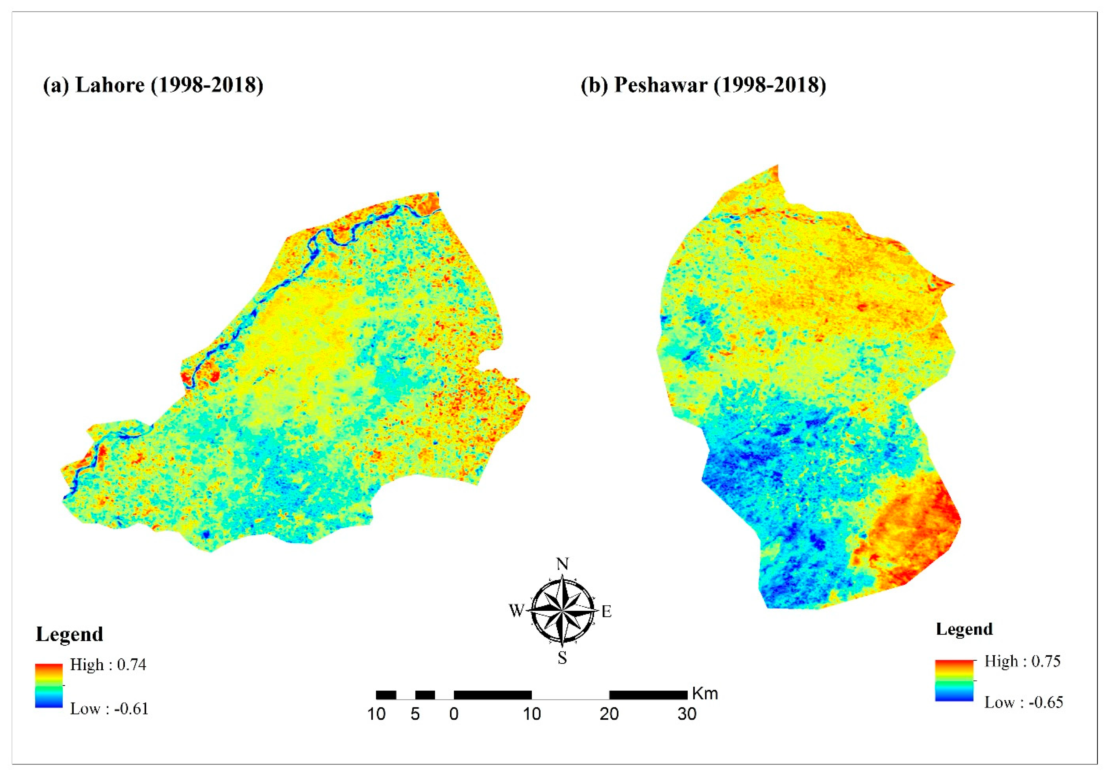
3.3. Land Surface Temperature (LST) Variations from 1998–2018

The LST patterns for Lahore and Peshawar for three months (May-July) in the years 1998, 2003, 2008, 2013 and 2018 were calculated as described in Section 2.3. Figure 7a shows the increase in the three-months averaged (May- July) LST in Lahore city during these 20 years. Both the minimum and maximum LSTs are higher in 2018 than in 1998, with maximum LST values of 35.31, 37.63, 38.87, 40.73 and 41.39 °C for 1998, 2003, 2008, 2013 and 2018, respectively. For these years, the minimum LST values were 18.56, 20.69, 21.11, 21.88 and 23.54 °C.

In contrast, Figure 7b indicates that in Peshawar city the LST has decreased during the study period, for both the minimum and maximum values. For the years 1998, 2003, 2008, 2013 and 2018 the maximum LST was 40.65, 37.37, 35.48, 36.17 and 34.05 °C, respectively, with a similar tendency for the minimum LST values which were 21.44, 20.22, 18.38, 18.66 and 17.84 °C for the years 1998, 2003, 2008, 2013 and 2018.

3.4. Correlation between LST and T (Air)

For evaluation of the Landsat-derived LST trend, it is compared to the corresponding 3 months (May–July) air temperatures (Ta) measured at meteorological stations in Lahore and Peshawar (

Table 9. Comparison of 3 months (May-July) of mean LST and air temperature T(a) in Lahore (top) and Peshawar (bottom).

Study Region	Year	Latitude	Longitude	T(a) °C	LST °C
Lahore city	1998	31.35	74.24	31.7	34.7
	2003	31.35	74.24	31.8	35.8
	2008	31.35	74.24	32.3	36.4
	2013	31.35	74.24	32.9	36.9
	2018	31.35	74.24	33.5	37.8
Peshawar city	1998	71.56	327.56	32.5	37.6
	2003	71.56	327.56	31.92	36.9
	2008	71.56	327.56	30.78	35.1
	2013	71.56	327.56	31.02	35.8
	2018	71.56	327.56	30.12	32.3

). The data in Table 9 show the increase in both LST and air temperature in Lahore, whereas in Peshawar, both the air temperature and the LST decrease during the study period.

The correlation of 3 months (May–July) of mean LST and air temperature T (a). The results in Figure 8 and Figure 9 show a good comparison with high correlation coefficients between LST and Ta.

3.5. Changes in LST in Response to Different Land-Use Classes

The change in LST in response to the transformation between different land-use classes was studied by determining relationships between LULC transition from 1998 to 2018 and LST using the curve fit tool and zonal statistic in ArcGIS (Section 2.6).

The results presented in

Table 10. Average contribution rate of LULC class transition to LST (°C) from 1998 to 2018.

Study Region	LU Classes	Water	Vegetation	Built-Up	Barren
Lahore city	Water	0.1	0.08	0.13	0.14
	Vegetation	−0.09	0.1	0.17	0.16
	Built-up	−0.11	−0.19	0.19	0.17
	Barren	−0.01	−0.19	0.16	0.06
Peshawar city	Water	0.1	−0.20	0.36	0.26
	Vegetation	−0.05	0.1	0.32	0.31
	Built-up	−0.13	−0.25	0.26	0.21
	Barren	−0.13	−0.27	0.25	0.09

and Figure 10 show the correlation between LST and LULC, i.e., the regression coefficient (r). The average change in LST (°C) from 1998 to 2018 due to the transitions between the four different LULC classes is presented in Table 10 for each type of change: the transition from built-up and barren land to vegetation and water cover results in a decrease in LST, whereas a change from water or vegetation cover to built-up or barren land results in an increase in LST. The results presented in Table 10 show that in Peshawar city, the LST was reduced by 0.25 and 0.27 °C in response to the transition from built-up and barren land to vegetation, respectively. In contrast, in Lahore city, the LST increased by 0.17 °C in response to the transition from vegetation to buildup land and 0.13 °C in response to the transition from water cover to built-up area.

4. Discussion

This research was carried out to quantify the individual contribution of different LULC transformations to LST in Lahore and Peshawar city (metropolitan areas of Pakistan) from 1998-2018, and future predictions of LULC for 2023 and 2028 by using CA-Markov model. Figure 3a highlights the land cover pattern for Lahore city and shows that the area covered by water bodies, vegetation, and barren land decreased gradually from 1998 to 2018, while built-up area increased. In Lahore city, the area covered by water bodies, vegetation, and barren land was 2.7%, 24.9% and 42.5% in 1998, which decreased to 0.6%, 22.6% and 35.7% in 2018, while built-up land gradually increased from 29.8% in 1998 to 41% in 2018, due to the transformation of different land-use categories into built-up areas. These conversions were mainly due to different housing and other projects by the Lahore Development Authority (LDA) and local developers [68,69], mega-development projects (including Metro Bus, Orange Train) [68,69,100].

However, Figure 3b shows, in Peshawar city, that the area covered by water, vegetation, and built-up land was about 1.8%, 25.0%, and 68.1%, respectively in 1998, and gradually increased to 2.4%, 50.6% and 21.5% in 2018. Barren land was found to decrease gradually with a higher rate (from 68.1% to 25.5%) due to its transformation into other land use classes. The increase in vegetation area was promoted by the “Billion trees project” (2013) of the KPK local government [72]. The increase in built-up area was needed because of bulk migration of people from Afghanistan toward the KPK Province in 2000–2005 during war-time [70].

Changes in the LULC also cause changes in the temperature [73,74], because different classes of LULC have different properties of reflectance and evapotranspiration [101]. Results of LST (Figure 7) indicate that in Lahore city during these 20 years, both the minimum and maximum LSTs are higher in 2018 than in 1998. These data confirm the results from earlier studies indicating that the LST rises in Lahore city [101,102], which may be due to the increasing use of artificial materials, such as asphalt and concrete, for urban expansion [103,104]. Our results from Figure 3a highlight that in Lahore city, the built-up area is increasing. The LST increases with the increase in urban built-up and barren land [105]. Meanwhile, in Peshawar city, the LST has decreased during the study period, for both the minimum and maximum values. Our results from Figure 3b highlight that in Peshawar city, the vegetation cover of the city has gradually increased in 2018 compared to 1998. The increase in vegetation area was promoted by the “Billion trees project” (2013) of the KPK local government [72]. Conversion between different LULC classes, especially the transformation of vegetation into built-up land, can effectively influence the land surface temperature [8,9,10].

Climatological data can be developed for two kinds of surface temperatures: near-surface air temperature Ta and the skin temperature, or land surface temperature (LST) [106]. Ta is measured at official weather stations at 1.5 m above the surface with sensors protected from radiation and adequately ventilated [107]. Hence, LST and air temperature are different parameters that cannot be directly compared but do influence each other. For the evaluation of the LST, they were compared with Ta from station data. The results in Figure 8 and Figure 9 show a good comparison with high correlation coefficients between LST and Ta and confirm our LST trends.

Furthermore, the change in LST in response to the transformation between different land-use classes was studied by determining the relationships between LULC transition from 1998 to 2018 and LST using the Curve Fit tool and zonal statistic in ArcGIS (Section 2.6). The results indicate that the average change in LST (°C) from 1998 to 2018 due to the transitions between the four different LULC classes is presented in Table 10 for each type of change: the transition from built-up and barren land to vegetation and water cover results in a decrease in LST, while the transition from vegetation and water to built-up and barren land results in an increase in LST. LST variation can be associated with various factors including LULC transition, population growth, and urban expansion [108], because the surface reflectance and roughness of different LULC classes are different, and different LULC types have unique properties in terms of the emission, reflection and absorption of radiation [11,12]. The future predictions results indicate that urban growth in Lahore city continues, at the expense of vegetation and barren land (Table 8); these changes will also impact the LST because urban expansion has a profound impact on local and regional climate [108,109].

5. Conclusions

Land use land cover (LULC) in Lahore and Peshawar, Pakistan, was determined using Landsat data for selected dates with 5 year intervals between 1998 and 2018. The changes in LULC classes during these 20 years and their impacts on urban thermal environments were determined. Markov and CA-Markov models were used to predict future changes for 2023 and 2028. The results indicate that much of the barren and vegetation land in Lahore has been converted into the urbanized area. Additionally, Peshawar city has experienced an increase in the built-up area, but vegetation cover and water have replaced barren land, which significantly changed the adverse effects of urbanization observed in Lahore to cooling in Peshawar. The different LULC types have unique properties in terms of the emission, absorption and reflection of radiation. Therefore, the gradual urban expansion and other anthropogenic activities affect the surface temperature, which is reflected by the analysis of the LST in response to the transition between LULC classes. Conversion from water or vegetation into built-up or barren lands results in the increase in LST. Conversely, the transition of areas from built-up or barren land into vegetation or water has helped to lower LST. The LST in Lahore city has substantially increased, while the LST in Peshawar city has decreased over the 20 year study period.

The future scenarios indicate that severe environmental problems may be expected in Lahore city, whereas the future scenarios of Peshawar show a way to improve living conditions in an expanding city. These results indicate that Lahore policies are needed to control current environmental issues and avoid further increase in these problems. This research provides the necessary information to environmentalists and policymakers in developing greening strategies for megacities to minimize future eco-environmental threats.

References

1. Montgomery, M.R. The urban transformation of the developing world. Science 2008, 319, 761–764. [Google Scholar] [CrossRef] [Green Version]
2. Mitchell, L.; Moss, N.H.O. Urban Mobility in the 1st Century. NYU Rudin Center for Transportation Policy. 2012. Available online: https://wagner.nyu.edu/files/rudincenter/NYU-BMWi-Project_Urban_Mobility_Report_November_2012.pdf (accessed on 11 September 2020).
3. Buhaug, H.; Urdal, H. An urbanization bomb? Population growth and social disorder in cities. Glob. Environ. Chang. 2013, 23, 1–10. [Google Scholar] [CrossRef]
4. Dhar, R.B.; Chakraborty, S.; Chattopadhyay, R.; Sikdar, P.K. Impact of Land-Use/Land-Cover Change on Land Surface Temperature Using Satellite Data: A Case Study of Rajarhat Block, North 24-Parganas District, West Bengal. J. Indian Soc. Remote Sens. 2019, 47, 331–348. [Google Scholar] [CrossRef]
5. Choudhury, D.; Das, K.; Das, A. Assessment of land use land cover changes and its impact on variations of land surface temperature in Asansol-Durgapur Development Region. Egypt. J. Remote Sens. Space Sci. 2019, 22, 203–218. [Google Scholar] [CrossRef]
6. Das, S.; Angadi, D.P. Land use-land cover (LULC) transformation and its relation with land surface temperature changes: A case study of Barrackpore Subdivision, West Bengal, India. Remote Sens. Appl. Soc. Environ. 2020, 19, 100322. [Google Scholar] [CrossRef]
7. Ullah, S.; Ahmad, K.; Sajjad, R.U.; Abbasi, A.M.; Nazeer, A.; Tahir, A.A. Analysis and simulation of land cover changes and their impacts on land surface temperature in a lower Himalayan region. J. Environ. Manag. 2019, 245, 348–357. [Google Scholar] [CrossRef]
8. Hope, A.S.; Mcdowell, T.P. The Relationship between Surface-Temperature and a Spectral Vegetation Index of a Tallgrass Prairie—Effects of Burning and Other Landscape Controls. Int. J. Remote Sens. 1992, 13, 2849–2863. [Google Scholar] [CrossRef]
9. Julien, Y.; Sobrino, J.A.; Verhoef, W. Changes in land surface temperatures and NDVI values over Europe between 1982 and 1999. Remote Sens. Environ. 2006, 103, 43–55. [Google Scholar] [CrossRef]
10. Smith, R.C.G.; Choudhury, B.J. On the Correlation of Indexes of Vegetation and Surface-Temperature over South-Eastern Australia. Int. J. Remote Sens. 1990, 11, 2113–2120. [Google Scholar] [CrossRef]
11. Hou, G.; Zhang, H.; Wang, Y.; Qiao, Z.; Zhang, Z. Retrieval and Spatial Distribution of Land Surface Temperature in the Middle Part of Jilin Province Based on MODIS Data. Sci. Geogr. Sin. 2010, 30, 421–427. [Google Scholar]
12. Patz, J.A.; Campbell-Lendrum, D.; Holloway, T.; Foley, J.A. Impact of regional climate change on human health. Nature 2005, 438, 310–317. [Google Scholar] [CrossRef]
13. Solaimani, K.; Arekhi, M.; Tamartash, R.; Miryaghobzadeh, M. Land use/cover change detection based on remote sensing data (A case study; Neka Basin). Agric. Biol. J. N. Am. 2010, 1, 1148–1157. [Google Scholar] [CrossRef]
14. Omar, N.; Sanusi, S.A.M.; Hussin, W.M.W.; Samat, N.; Mohammed, K.S. Markov-CA model using analytical hierarchy process and multiregression technique. In IOP Conference Series: Earth and Environmental Science; IOP Publishing: Bristol, UK, 2014. [Google Scholar]
15. Kalnay, E.; Cai, M. Impact of urbanization and land-use change on climate. Nature 2003, 423, 528–531. [Google Scholar] [CrossRef]
16. Chen, X.L.; Zhao, H.-M.; Li, P.-X.; Yin, Z.-Y. Remote sensing image-based analysis of the relationship between urban heat island and land use/cover changes. Remote Sens. Environ. 2006, 104, 133–146. [Google Scholar] [CrossRef]
17. De Sherbinin, A. A CIESIN thematic guide to land-use and land-cover change (LUCC). In Center for International Earth Science Information Network; Columbia University: New York, NY, USA, 2002. [Google Scholar]
18. Eastman, J.; Van Fossen, M.; Solarzano, L. Transition potential modeling for land cover change. GIS Spat. Anal. Model. 2005, 357–386. [Google Scholar]
19. Rai, R.; Zhang, Y.; Paudel, B.; Li, S.; Khanal, N.R. A Synthesis of Studies on Land Use and Land Cover Dynamics during 1930-2015 in Bangladesh. Sustainability 2017, 9, 1866. [Google Scholar] [CrossRef] [Green Version]
20. Briassoulis, H. Analysis of Land Use Change: Theoretical and Modeling Approaches; Regional Research Institute, West Virginia University: Morgantown, WV, USA, 2019. [Google Scholar]
21. Sun, C.; Wu, Z.-F.; Lv, Z.-Q.; Yao, N.; Wei, J.-B. Quantifying different types of urban growth and the change dynamic in Guangzhou using multi-temporal remote sensing data. Int. J. Appl. Earth Obs. Geoinf. 2013, 21, 409–417. [Google Scholar] [CrossRef]
22. Zhao, M.; Cheng, W.; Zhou, C.; Li, M.; Huang, K.; Wang, N. Assessing Spatiotemporal Characteristics of Urbanization Dynamics in Southeast Asia Using Time Series of DMSP/OLS Nighttime Light Data. Remote Sens. 2018, 10, 47. [Google Scholar] [CrossRef] [Green Version]
23. Lu, Q.; Chang, N.-B.; Joyce, J.; Chen, A.S.; Savić, D.; Djordjević, S.; Fu, G. Exploring the potential climate change impact on urban growth in London by a cellular automata-based Markov chain model. Comput. Environ. Urban Syst. 2018, 68, 121–132. [Google Scholar] [CrossRef]
24. BK, K. Internal Migration in Nepal: Population Monograph of Nepal 2003, II; Central Bureau of Statistics: Kathmandu, Nepal, 2003.
25. Seto, K.C.; Fragkias, M.; Güneralp, B.; Reilly, M.K. A meta-analysis of global urban land expansion. PLoS ONE 2011, 6, e23777. [Google Scholar] [CrossRef]
26. Bounoua, L.; Nigro, J.; Zhang, P.; Thome, K.; Lachir, A. Mapping urbanization in the United States from 2001 to 2011. Appl. Geogr. 2018, 90, 123–133. [Google Scholar] [CrossRef]
27. Pickard, B.R.; Van Berkel, D.B.; Petrasova, A.; Meentemeyer, R.K. Forecasts of urbanization scenarios reveal trade-offs between landscape change and ecosystem services. Landsc. Ecol. 2017, 32, 617–634. [Google Scholar] [CrossRef]
28. Lu, Y.T.; Wu, P.; Ma, X.; Li, X. Detection and prediction of land use/land cover change using spatiotemporal data fusion and the Cellular Automata-Markov model. Environ. Monit. Assess. 2019, 191, 68. [Google Scholar] [CrossRef]
29. Abdullahi, S.; Pradhan, B. Land use change modeling and the effect of compact city paradigms: Integration of GIS-based cellular automata and weights-of-evidence techniques. Environ. Earth Sci. 2018, 77, 251. [Google Scholar] [CrossRef]
30. Gessesse, B.; Bewket, W. Drivers and implications of land use and land cover change in the central highlands of Ethiopia: Evidence from remote sensing and socio-demographic data integration. Ethiop. J. Soc. Sci. Humanit. 2014, 10, 1–23. [Google Scholar]
31. Lambin, E.F.; Geist, H.J.; Lepers, E. Dynamics of land-use and land-cover change in tropical regions. Annu. Rev. Environ. Resour. 2003, 28, 205–241. [Google Scholar] [CrossRef] [Green Version]
32. Geist, H.; McConnell, W.; Lambin, E.F.; Moran, E.; Alves, D.; Rudel, T. Causes and trajectories of land-use/cover change. In Land-Use and Land-Cover Change; Springer: Berlin/Heidelberg, Germany, 2006; pp. 41–70. [Google Scholar]
33. Raza, A.; Raja, I.A.; Raza, S. Land-use change analysis of district Abbottabad, Pakistan: Taking advantage of GIS and remote sensing analysis. Sci. Vis. 2012, 18, 43–49. [Google Scholar]
34. Tao, S.; Yang, Y.; Zhang, A.-M.; Jiang, Y.; Xun, S.; Zhang, H. Study of Thermal Environment of Hefei City based on TM and GIS. Remote Sens. Technol. Appl. 2011, 26, 156–162. [Google Scholar]
35. Shi, T.; Yang, Y.; Ma, J.; Zhang, L.; Luo, S. Spatial temporal characteristics of urban heat island in typical cities of Anhui Province based on MODIS. J. Appl. Meteorol. Sci. 2013, 24, 484–494. [Google Scholar]
36. Wulder, M.A.; White, J.C.; Loveland, T.R.; Woodcock, C.E.; Belward, A.S.; Cohen, W.B.; Fosnight, E.A.; Shaw, J.; Masek, J.G.; Roy, D.P. The global Landsat archive: Status, consolidation, and direction. Remote Sens. Environ. 2016, 185, 271–283. [Google Scholar] [CrossRef] [Green Version]
37. Singh, S.K.; Mustak, S.; Srivastava, P.K.; Szabó, S.; Islam, T. Predicting spatial and decadal LULC changes through cellular automata Markov chain models using earth observation datasets and geo-information. Environ. Process. 2015, 2, 61–78. [Google Scholar] [CrossRef] [Green Version]
38. Hamad, R.; Balzter, H.; Kolo, K. Predicting Land Use/Land Cover Changes Using a CA-Markov Model under Two Different Scenarios. Sustainability 2018, 10, 3421. [Google Scholar] [CrossRef] [Green Version]
39. Moghadam, H.S.; Helbich, M. Spatiotemporal urbanization processes in the megacity of Mumbai, India: A Markov chains-cellular automata urban growth model. Appl. Geogr. 2013, 40, 140–149. [Google Scholar] [CrossRef]
40. Wu, D.Q.; Liu, J.; Wang, S.; Wang, R. Simulating urban expansion by coupling a stochastic cellular automata model and socioeconomic indicators. Stoch. Environ. Res. Risk Assess. 2010, 24, 235–245. [Google Scholar] [CrossRef]
41. Batty, M.; Xie, Y. Urban Growth Using Cellular Automata Models; ESRI Press: Redlands, CA, USA, 2005. [Google Scholar]
42. Mas, J.F.; Kolb, M.; Paegelow, M.; Olmedo, M.T.C.; Houet, T. Inductive pattern-based land use/cover change models: A comparison of four software packages. Environ. Model. Softw. 2014, 51, 94–111. [Google Scholar] [CrossRef] [Green Version]
43. Nadeem, F. Monitoring Urbanization and Comparison with City Master Plans using Remote Sensing and GIS: A Case Study of Lahore District, Pakistan. Int. J. Adv. Remote Sens. GIS 2017, 6, 2234–2245. [Google Scholar] [CrossRef]
44. Kityuttachai, K.; Tripathi, N.K.; Tipdecho, T.; Shrestha, R.P. CA-Markov Analysis of Constrained Coastal Urban Growth Modeling: Hua Hin Seaside City, Thailand. Sustainability 2013, 5, 1480–1500. [Google Scholar] [CrossRef] [Green Version]
45. García, A.; Santé, I.; Boullón, M.; Crecente, R. Calibration of an urban cellular automaton model by using statistical techniques and a genetic algorithm. Application to a small urban settlement of NW Spain. Int. J. Geogr. Inf. Sci. 2013, 27, 1593–1611. [Google Scholar] [CrossRef]
46. Maithani, S. Cellular Automata Based Model of Urban Spatial Growth. J. Indian Soc. Remote Sens. 2010, 38, 604–610. [Google Scholar] [CrossRef]
47. Nouri, J.; Gharagozlou, A.; Arjmandi, R.; Faryadi, S.; Adl, M. Predicting Urban Land Use Changes Using a CA-Markov Model. Arab. J. Sci. Eng. 2014, 39, 5565–5573. [Google Scholar] [CrossRef]
48. Ke, X.L.; Qi, L.Y.; Zeng, C. A partitioned and asynchronous cellular automata model for urban growth simulation. Int. J. Geogr. Inf. Sci. 2016, 30, 637–659. [Google Scholar] [CrossRef]
49. Akın, A.; Sunar, F.; Berberoğlu, S. Urban change analysis and future growth of Istanbul. Environ. Monit. Assess. 2015, 187, 506. [Google Scholar] [CrossRef]
50. Guan, D.; Li, H.; Inohae, T.; Su, W.; Nagaie, T.; Hokao, K. Modeling urban land use change by the integration of cellular automaton and Markov model. Ecol. Model. 2011, 222, 3761–3772. [Google Scholar] [CrossRef]
51. Kamusoko, C.; Aniya, M.; Adi, B.; Manjoro, M. Rural sustainability under threat in Zimbabwe–simulation of future land use/cover changes in the Bindura district based on the Markov-cellular automata model. Appl. Geogr. 2009, 29, 435–447. [Google Scholar] [CrossRef]
52. Steeb, W.-H. The Nonlinear Workbook: Chaos, Fractals, Cellular Automata, Genetic Algorithms, Gene Expression Programming, Support Vector Machine, Wavelets, Hidden Markov Models, Fuzzy Logic with C++; World Scientific Publishing Company: Singapore, 2014. [Google Scholar]
53. Riccioli, F.; El Asmar, T.; El Asmar, J.-P.; Fratini, R. Use of cellular automata in the study of variables involved in land use changes. Environ. Monit. Assess. 2013, 185, 5361–5374. [Google Scholar] [CrossRef]
54. Roose, M.; Hietala, R. A methodological Markov-CA projection of the greening agricultural landscape-a case study from 2005 to 2017 in southwestern Finland. Environ. Monit. Assess. 2018, 190, 411. [Google Scholar] [CrossRef]
55. Arsanjani, J.J.; Helbich, M.; Kainz, W.; Boloorani, A.D. Integration of logistic regression, Markov chain and cellular automata models to simulate urban expansion. Int. J. Appl. Earth Obs. Geoinf. 2013, 21, 265–275. [Google Scholar] [CrossRef]
56. Keshtkar, H.; Voigt, W. A spatiotemporal analysis of landscape change using an integrated Markov chain and cellular automata models. Modeling Earth Syst. Environ. 2016, 2, 10. [Google Scholar] [CrossRef] [Green Version]
57. Rimal, B.; Zhang, L.; Keshtkar, H.; Wang, N.; Lin, Y. Monitoring and Modeling of Spatiotemporal Urban Expansion and Land-Use/Land-Cover Change Using Integrated Markov Chain Cellular Automata Model. Isprs Int. J. Geo-Inf. 2017, 6, 288. [Google Scholar] [CrossRef] [Green Version]
58. Araya, Y.H.; Cabral, P. Analysis and Modeling of Urban Land Cover Change in Setubal and Sesimbra, Portugal. Remote Sens. 2010, 2, 1549–1563. [Google Scholar] [CrossRef] [Green Version]
59. Munshi, T.; Zuidgeest, M.; Brussel, M.; Van Maarseveen, M. Logistic regression and cellular automata-based modelling of retail, commercial and residential development in the city of Ahmedabad, India. Cities 2014, 39, 68–86. [Google Scholar] [CrossRef]
60. Puertas, O.L.; Henríquez, C.; Meza, F.J. Assessing spatial dynamics of urban growth using an integrated land use model. Application in Santiago Metropolitan Area, 2010–2045. Land Use Policy 2014, 38, 415–425. [Google Scholar] [CrossRef]
61. Han, Y.; Jia, H.F. Simulating the spatial dynamics of urban growth with an integrated modeling approach: A case study of Foshan, China. Ecol. Model. 2017, 353, 107–116. [Google Scholar] [CrossRef]
62. Nasir, M.J.; Tabassum, I.; Khan, A.S.; Alam, S. Land Use Temporal Changes: A Comparison Using Field Survey and Remote Sensing.(A Case Study of Killi Kambarani & Satellite Town, Quetta City). Putaj Sci. 2012, 19, 91–106. [Google Scholar]
63. Li, X.; Yeh, A.G.O. Modelling sustainable urban development by the integration of constrained cellular automata and GIS. Int. J. Geogr. Inf. Sci. 2000, 14, 131–152. [Google Scholar] [CrossRef]
64. Foley, J.A.; DeFries, R.; Asner, G.P.; Barford, C.; Bonan, G.; Carpenter, S.R.; Chapin, F.S.; Coe, M.T.; Daily, G.C.; Gibbs, H.K.; et al. Global consequences of land use. Science 2005, 309, 570–574. [Google Scholar] [CrossRef] [Green Version]
65. Wu, K.-Y.; Zhang, H. Land use dynamics, built-up land expansion patterns, and driving forces analysis of the fast-growing Hangzhou metropolitan area, eastern China (1978–2008). Appl. Geogr. 2012, 34, 137–145. [Google Scholar] [CrossRef]
66. Dubovyk, O.; Sliuzas, R.; Flacke, J. Spatio-temporal modelling of informal settlement development in Sancaktepe district, Istanbul, Turkey. ISPRS J. Photogramm. Remote Sens. 2011, 66, 235–246. [Google Scholar] [CrossRef]
67. Poelmans, L.; van Rompaey, A. Detecting and modelling spatial patterns of urban sprawl in highly fragmented areas: A case study in the Flanders–Brussels region. Landsc. Urban Plan. 2009, 93, 10–19. [Google Scholar] [CrossRef]
68. Shah, B.; Ghauri, B. Mapping urban heat island effect in comparison with the land use, land cover of Lahore district. Pak. J. Meteorol. Vol 2015, 11, 1–12. [Google Scholar]
69. Nespak, L. Integrated Master Plan for Lahore-2021; Lahore Development Authority: Lahore, Pakistan, 2004. [Google Scholar]
70. Raziq, A.; Xu, A.; Li, Y.; Zhao, Q. Monitoring of land use/land cover changes and urban sprawl in Peshawar City in Khyber Pakhtunkhwa: An application of geo-information techniques using of multi-temporal satellite data. J. Remote Sens. GIS 2016, 5, 174. [Google Scholar] [CrossRef]
71. Mehmood, R.; Mehmood, S.A.; Butt, M.A.; Younas, I.; Adrees, M. Spatiotemporal analysis of urban sprawl and its contributions to climate and environment of Peshawar using remote sensing and GIS techniques. J. Geogr. Inf. Syst. 2016, 8, 137–148. [Google Scholar] [CrossRef] [Green Version]
72. Khan, N.; Shah, S.J.; Rauf, T.; Zada, M.; Cao, Y.; Harbi, J. Socioeconomic Impacts of the Billion Trees Afforestation Program in Khyber Pakhtunkhwa Province (KPK), Pakistan. Forests 2019, 10, 703. [Google Scholar] [CrossRef] [Green Version]
73. Goksel, C.; Mercan, D.; Kabdasli, S.; Bektas, F.; Seker, D.Z. Definition of sensitive areas in a lakeshore by using remote sensing and GIS. Fresenius Environ. Bull. 2004, 13, 860–864. [Google Scholar]
74. Goksel, C.; Musaoglu, N.; Gurel, M.; Ulugtekin, N.; Tanik, A.G.; Seker, D.Z. Determination of land-use change in an urbanized district of Istanbul via remote sensing analysis. Fresenius Environ. Bull. 2006, 15, 798–805. [Google Scholar]
75. Bhatti, S.S.; Tripathi, N.K. Built-up area extraction using Landsat 8 OLI imagery. GISci. Remote Sens. 2014, 51, 445–467. [Google Scholar] [CrossRef] [Green Version]
76. Deng, C.; Wu, C. A spatially adaptive spectral mixture analysis for mapping subpixel urban impervious surface distribution. Remote Sens. Environ. 2013, 133, 62–70. [Google Scholar] [CrossRef]
77. Jiménez-Muñoz, J.C.; Sobrino, J.A. A generalized single-channel method for retrieving land surface temperature from remote sensing data. J. Geophys. Res. Atmos. 2003, 108, 4688. [Google Scholar] [CrossRef] [Green Version]
78. Qin, Z.; Karnieli, A.; Berliner, P. A mono-window algorithm for retrieving land surface temperature from Landsat TM data and its application to the Israel-Egypt border region. Int. J. Remote Sens. 2001, 22, 3719–3746. [Google Scholar] [CrossRef]
79. Sultana, S.; Satyanarayana, A. Urban heat island intensity during winter over metropolitan cities of India using remote-sensing techniques: Impact of urbanization. Int. J. Remote Sens. 2018, 39, 6692–6730. [Google Scholar] [CrossRef]
80. Karakus, C.B.; Kavak, K.S.; Cerit, O. Determination of variations in land cover and land use by remote sensing and geographic information systems around the city of Sivas (Turkey). Fresenius Environ. Bull. 2014, 23, 667–677. [Google Scholar] [CrossRef] [Green Version]
81. Asmala, A. Analysis of maximum likelihood classification on multispectral data. Appl. Math. Sci. 2012, 6, 6425–6436. [Google Scholar]
82. Zhang, H.; Qi, Z.-F.; Ye, X.-Y.; Cai, Y.; Ma, W.-C.; Chen, M.-N. Analysis of land use/land cover change, population shift, and their effects on spatiotemporal patterns of urban heat islands in metropolitan Shanghai, China. Appl. Geogr. 2013, 44, 121–133. [Google Scholar] [CrossRef]
83. Arshad, A.; Zhang, W.; Zaman, M.A.; Dilawar, A.; Sajid, Z. Monitoring the impacts of spatio-temporal land-use changes on the regional climate of city Faisalabad, Pakistan. Ann. GIS 2019, 25, 57–70. [Google Scholar] [CrossRef] [Green Version]
84. Fatemi, M.; Narangifard, M. Monitoring LULC changes and its impact on the LST and NDVI in District 1 of Shiraz City. Arabian J. Geosci. 2019, 12, 1–12. [Google Scholar] [CrossRef]
85. Chander, G.; Markham, B.L.; Helder, D.L. Summary of current radiometric calibration coefficients for Landsat MSS, TM, ETM+, and EO-1 ALI sensors. Remote Sens. Environ. 2009, 113, 893–903. [Google Scholar] [CrossRef]
86. Sekertekin, A.; Kutoglu, S.H.; Kaya, S. Evaluation of spatio-temporal variability in Land Surface Temperature: A case study of Zonguldak, Turkey. Environ. Monit. Assess. 2016, 188, 30. [Google Scholar] [CrossRef]
87. Bhalli, M.; Ghaffar, A.; Shirazi, S.A.; Parveen, N.; Anwar, M.M. Change detection analysis of land use by using geospatial techniques: A case study of Faisalabad-Pakistan. Sci. Int. 2012, 24, 539–546. [Google Scholar]
88. Nichol, J.E. A GIS-based approach to microclimate monitoring in Singapore’s high-rise housing estates. Photogramm. Eng. Remote Sens. 1994, 60, 1225–1232. [Google Scholar]
89. Du, P.; Li, X.; Cao, W.; Luo, Y.; Zhang, H. Monitoring urban land cover and vegetation change by multi-temporal remote sensing information. Min. Sci. Technol. 2010, 20, 922–932. [Google Scholar] [CrossRef]
90. Burnham, B.O. Markov intertemporal land use simulation model. J. Agric. Appl. Econ. 1973, 5, 253–258. [Google Scholar] [CrossRef] [Green Version]
91. Subedi, P.; Subedi, K.; Thapa, B. Application of a hybrid cellular automaton–Markov (CA-Markov) model in land-use change prediction: A case study of Saddle Creek Drainage Basin, Florida. Appl. Ecol. Environ. Sci. 2013, 1, 126–132. [Google Scholar] [CrossRef] [Green Version]
92. Fathizad, H.; Rostami, N.; Faramarzi, M. Detection and prediction of land cover changes using Markov chain model in semi-arid rangeland in western Iran. Environ. Monit. Assess. 2015, 187, 629. [Google Scholar] [CrossRef] [PubMed]
93. Wang, S.; Zhang, Z.; Wang, X. Land use change and prediction in the Baimahe Basin using GIS and CA-Markov model. In IOP Conference Series: Earth and Environmental Science; IOP Publishing: Bristol, UK, 2014. [Google Scholar]
94. Halmy, M.W.A.; Gessler, P.E.; Hicke, J.A.; Salem, B. Land use/land cover change detection and prediction in the north-western coastal desert of Egypt using Markov-CA. Appl. Geogr. 2015, 63, 101–112. [Google Scholar] [CrossRef]
95. Mitsova, D.; Shuster, W.; Wang, X. A cellular automata model of land cover change to integrate urban growth with open space conservation. Landsc. Urban Plan. 2011, 99, 141–153. [Google Scholar] [CrossRef]
96. Santé, I.; García, A.M.; Miranda, D.; Crecente, R. Cellular automata models for the simulation of real-world urban processes: A review and analysis. Landsc. Urban Plan. 2010, 96, 108–122. [Google Scholar] [CrossRef]
97. Kumar, S.; Radhakrishnan, N.; Mathew, S. Land use change modelling using a Markov model and remote sensing. Geomat. Nat. Hazards Risk 2014, 5, 145–156. [Google Scholar] [CrossRef]
98. Lillesand, T.; Kiefer, R.W.; Chipman, J. Remote Sensing and Image Interpretation; John Wiley & Sons: Hoboken, NJ, USA, 2015. [Google Scholar]
99. Shawul, A.A.; Chakma, S. Spatiotemporal detection of land use/land cover change in the large basin using integrated approaches of remote sensing and GIS in the Upper Awash basin, Ethiopia. Environ. Earth Sci. 2019, 78, 141. [Google Scholar] [CrossRef]
100. Lahore Development Authority (LDA). Available online: https://www.lda.gop.pk (accessed on 13 July 2020).
101. Nasar-u-Minallah, M. Retrieval of land surface temperature of Lahore through Landsat-8 TIRS data. Int. J. Econ. Environ. Geol. 2019, 10, 70–77. [Google Scholar] [CrossRef]
102. Mumtaz, F.; Tao, Y.; Bashir, B.; Ahmad, A.; Li, L.; Hassan, H.U. The relationship between vegetation dynamics and land surface temperature by using different satellite imageries; A Case study of Metropolitan cities of Pakistan. N. Am. Acad. Res. 2020, 3, 1–15. [Google Scholar] [CrossRef]
103. Hallegatte, S.; Corfee-Morlot, J. Understanding climate change impacts, vulnerability and adaptation at city scale: An introduction. Clim. Chang. 2011, 104, 1–12. [Google Scholar] [CrossRef]
104. Kant, Y.; Bharath, B.D.; Mallick, J.; Atzberger, C.; Kerle, N. Satellite-based analysis of the role of land use/land cover and vegetation density on surface temperature regime of Delhi, India. J. Indian Soc. Remote Sens. 2009, 37, 201–214. [Google Scholar] [CrossRef]
105. Sun, Q.Q.; Wu, Z.F.; Tan, J.J. The relationship between land surface temperature and land use/land cover in Guangzhou, China. Environ. Earth Sci. 2012, 65, 1687–1694. [Google Scholar] [CrossRef]
106. Jin, M.; Dickinson, R.E. Land surface skin temperature climatology: Benefitting from the strengths of satellite observations. Environ. Res. Lett. 2010, 5, 044004. [Google Scholar] [CrossRef] [Green Version]
107. Karl, T.; Hassol, S.J.; Miller, C.D.; Murray, W.L. Temperature Trends in the Lower Atmosphere: Steps for Understanding and Reconciling Differences; A Report by the Climate Change Science Program and Subcommittee on Global Change Research; Climate Change Science Program: Washington, DC, USA, 2006; 180p. [Google Scholar]
108. Jiang, J.; Tian, G. Analysis of the impact of land use/land cover change on land surface temperature with remote sensing. Procedia Environ. Sci. 2010, 2, 571–575. [Google Scholar] [CrossRef] [Green Version]
109. Khan, I.; Zhao, M. Water resource management and public preferences for water ecosystem services: A choice experiment approach for inland river basin management. Sci. Total Environ. 2019, 646, 821–831. [Google Scholar] [CrossRef]
Figure 1. Map of the study area.
Remotesensing 12 02987 g001
Figure 2. Flow chart visualizing the data preprocessing and analysis methodology.
Remotesensing 12 02987 g002
Figure 3. Spatial patterns of land use land cover (LULC) in Lahore (a) and Peshawar (b).
Remotesensing 12 02987 g003
Figure 4. Transition between LULC classes (1998–2018) for Lahore and Peshawar city.
Remotesensing 12 02987 g004
Figure 5. Comparison of LULC maps for Lahore and Peshawar for 2013, predicted using the CA-Markov model with the satellite-derived LULC maps.
Remotesensing 12 02987 g005
Figure 6. LULC predictions for 2023 and 2028 for Lahore city and Peshawar city.
Remotesensing 12 02987 g006
Figure 7. Spatial patterns of land surface temperature (LST, °C) in Lahore (a) and Peshawar (b), averaged over 3 months (May–July), for each study year.
Remotesensing 12 02987 g007
Figure 8. Scatterplot of LST versus Ta (3 months average (May–July) for Lahore city.
Remotesensing 12 02987 g008
Figure 9. As Figure 8, for Peshawar city.
Remotesensing 12 02987 g009
Figure 10. Regression coefficients (see color scales) between LST and LULC class transition in (a) Lahore and (b) Peshawar from 1998 to 2018.
Remotesensing 12 02987 g010