1. Introduction
Ionospheric delay is one of the main error sources in the positioning and navigation applications of global navigation satellite systems (GNSSs) [
1,
2,
3,
4]. Under normal solar activity, the ionospheric delay is usually up to tens of meters, but it may exceed more than 100 m with ionospheric scintillation. Over the past two decades, the international GNSS Service (IGS) ionospheric working group has routinely produced global ionospheric map products with the developing GNSS constellations and installation of ground-based GNSS receiver sites worldwide [
5]. For ionosphere modeling, the influence of the ionospheric layer height in the thin layer ionospheric model is investigated [
6] and an enhanced mapping function is proposed [
7]. An improved empirical model is used for ionosphere modeling, considering the stochastic process of each satellite [
8]. The higher-order ionospheric delay is also demonstrated to mitigate its effects on precise point positioning (PPP) during disturbed ionospheric conditions [
9]. The two-layer ionospheric model is also proposed to better model the structure of the ionosphere [
10]. Consequently, the different ionospheric models are demonstrated to assess their performance in single-frequency or multi-frequency PPP [
11,
12,
13,
14]. The real-time ionospheric delays corrections are used in faster PPP to shorten the convergence time and obtain the fixed-ambiguities solutions [
15,
16,
17].
To establish the ionospheric modeling with GNSS, extraction of ionospheric observables is the first task [
18,
19,
20]. Due to the frequency-dependent features, the ionospheric information obtained from GNSS technology is coupled with satellite and receiver differential code biases (DCBs) [
21,
22]. Consequently, the DCBs interferes with the estimation of accurate and absolute ionospheric total electron content (TEC), and the performance of positioning and timing. The geometry-free (GF) combination of carrier-phase smoothed code measurements, which is applied by the CODE, is commonly used to estimate the ionospheric observables [
23]. The carrier-to-code leveling (CCL) method with carrier-phase smoothed code measurements reduces the code noise by an averaging process and avoids resolving ambiguities. However, the leveling errors, a type of error related to arcs created due to the multipath and short-term fluctuation of receiver biases, degrades the accuracy of ionospheric observables [
22,
24,
25].
Due to the high precision of precise point positioning (PPP), the ionospheric observables can be directly extracted by the uncombined PPP (UPPP) method [
26,
27]. In [
28], the UPPP method was used to avoid the leveling errors by using precise ambiguity estimation and multipath effects elimination. In [
18], the real-time ionospheric total electron content (TEC) was monitored and modeled by the UPPP method, and an accuracy of 1 to 2 TECU (Total Electron Content Unit) and 0.4 ns for ionosphere and DCBs results was achieved, respectively.
Significant receiver DCB seasonal variations, which are correlated with the ambient environment, have been found [
29], excepting the reason of solar cycle variability [
30]. Furthermore, the strong correlation between the total electron content (TEC) and receiver DCB stability was demonstrated during a three-year period [
31]. Receiver DCBs are not as stable as the GNSS transmitter DCBs and sometimes remarkable intraday variability is exhibited in leveling errors of ionospheric observables [
32,
33]. The short-term variation of receiver code bias is also presented on the leveling errors of a short baseline [
19,
26]. This variation is caused by many factors, for instance, the grounding of GPS equipment [
34] and the environment temperature [
32]. To eliminate the time-variating terms of receiver DCBs, a modified carrier-to-code leveling method is proposed to retrieve ionospheric observables [
25]. A detailed study of receiver DCBs’ short-term variability should be done with high precision ionospheric observables.
In previous research, the ionospheric observables for ionosphere modeling and DCB estimation are based on the smoothed ambiguities or float-ambiguity solutions [
18,
28]. The double-difference fixed-ambiguity solutions are used to extract the precise ionospheric observables in regional ionosphere modeling [
35]. The PPP AR has already achieved by the decoupled satellite clock (DSC) model [
36], fractional cycle bias (FCB) model [
37,
38], and the integer recovery clock model [
39]. An “integer-levelling” method, which attempted to fix the ambiguity with integer values from the carrier-phase smoothed code method using decoupled-clock products, was proposed to eliminate the leveling errors [
40,
41,
42]. The FCB model is also adopted to fix geometry-free combination ambiguities with wide-lane fixed-ambiguity and ionospheric-free fixed-ambiguity ionospheric extraction [
10,
43,
44]. However, these methods are also based on the CCL method with geometry-free carrier-phase observations. Compared with the above methods, the UPPP method is more flexible in estimating the precise ionospheric observables with ambiguity-fixed solutions, which can evidently reduce the leveling error effects of ionospheric observables. The reliable ambiguity resolution is a key issue to obtain precise ionospheric observables. However, less studies have been based on the ambiguity-fixed uncombined PPP.
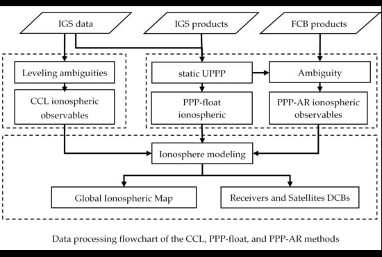
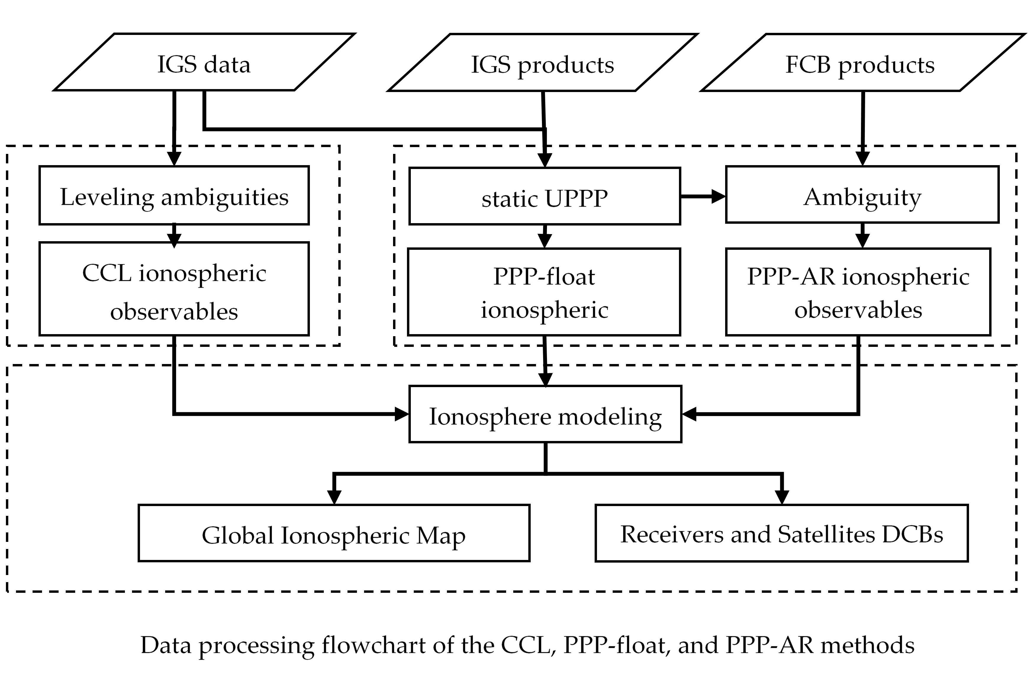
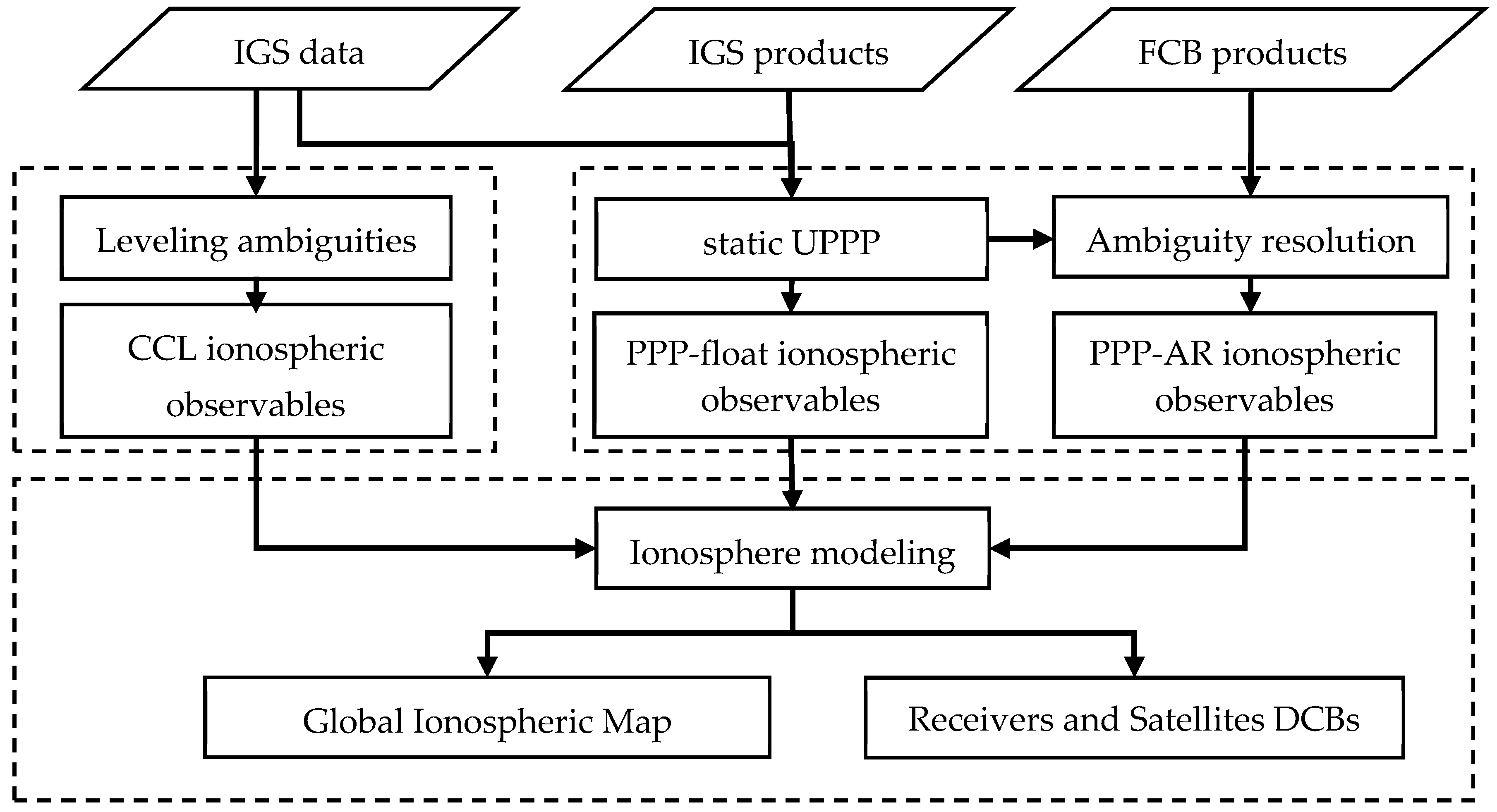
In this study, we firstly present the mathematical models to estimate the ionospheric observables with the CCL and PPP method. The ambiguity resolution method, ionospheric modeling, and DCB estimation method are also presented. Thereafter, the data process strategy is introduced. The ionospheric observables were estimated with the CCL, PPP float-ambiguity, and PPP fixed-ambiguity solution methods, respectively. Three comprehensive global ionospheric map (GIM) products were produced. Then, the comprehensive analyzes of the accuracy of three GIM products were performed. Finally, we discuss the results and give some conclusions.
4. Discussion
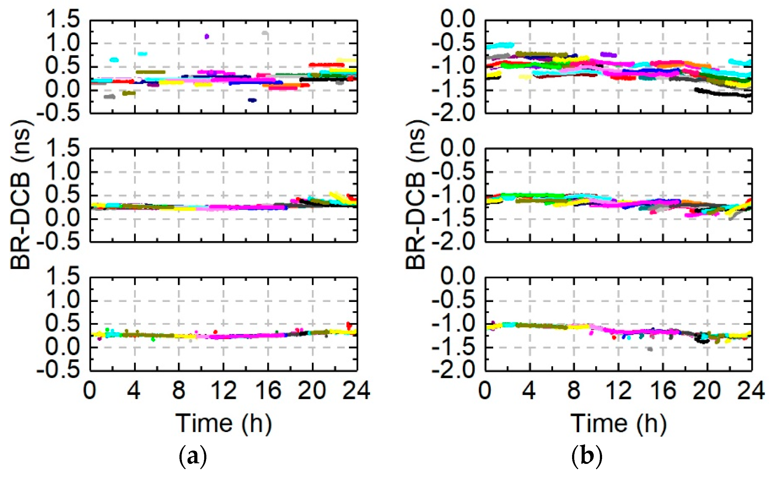
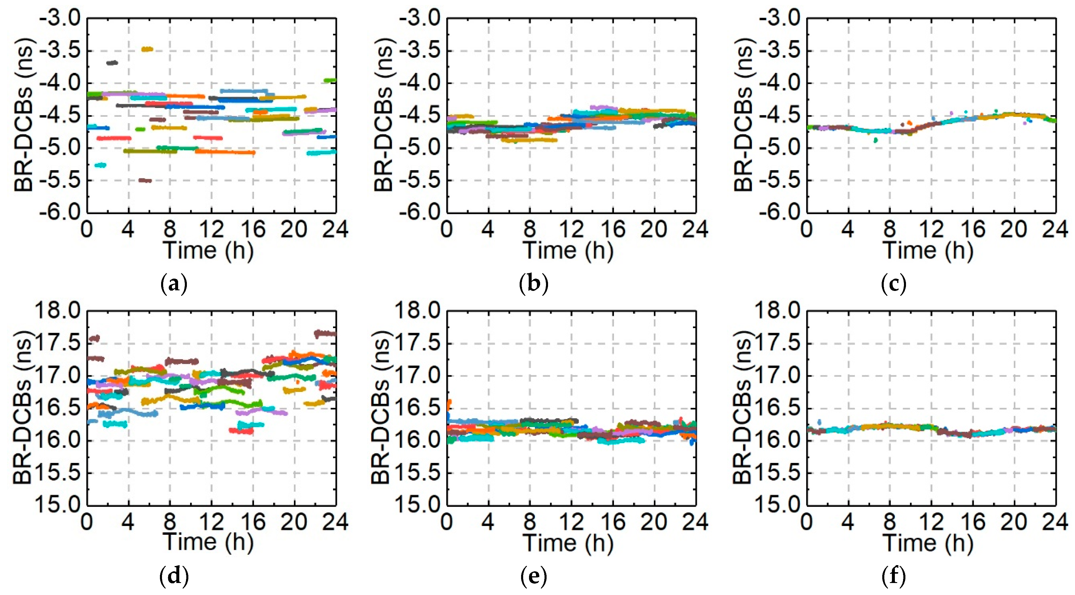
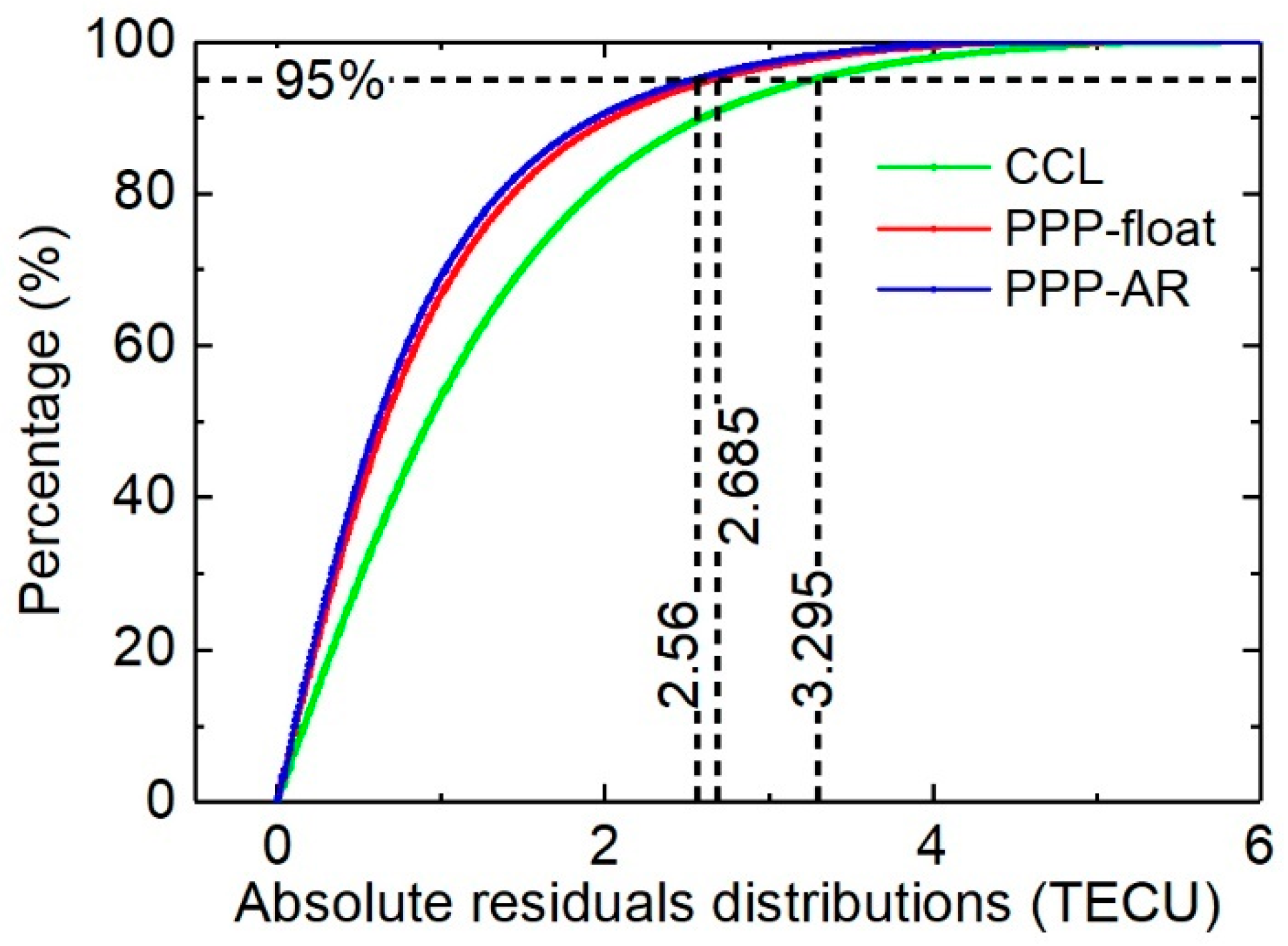
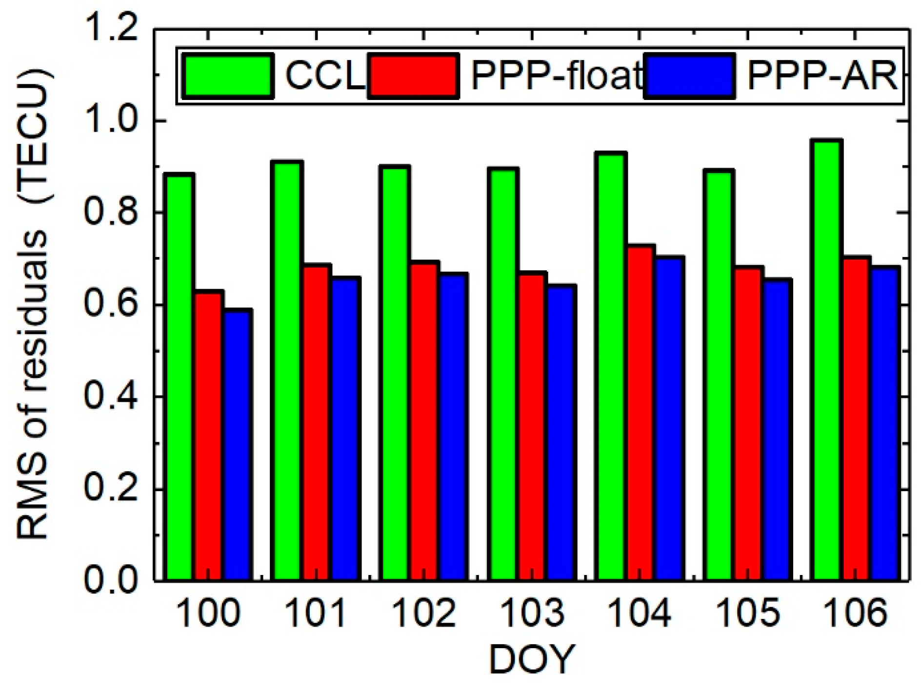
The main interest of this study was the accuracy assessment of ionospheric observables obtained from the uncombined PPP with fixed ambiguity resolution and the corresponding ionosphere modeling. Excepting that the ionosphere modeling resolution can affect the performance, the measurement errors of ionospheric observables in reference stations is the main limitation in global ionospheric map corrections. The accuracy of ionospheric observables obtained from the CCL, PPP-float, and PPP-AR methods was firstly assessed by zero and short baseline experiments. With the fixed ambiguity resolution, the STD of single-differenced ionospheric observables is only about a quarter of that for CCL method. Compared with PPP-float solutions, 30.7% improvements were achieved for PPP-AR solutions. The undifferenced and uncombined PPP with fixed ambiguity resolution not only improves the performance of positioning but also improves the accuracy of ionosphere parameter estimation. For epoch solutions, the accuracy of ionospheric observables from PPP methods, removing the effects of the arc length and code measurement noise, is better than that of the CCL method. With high precision ionospheric observables, the slight variations of receiver DCBs is legible for an analysis of the receiver performances.
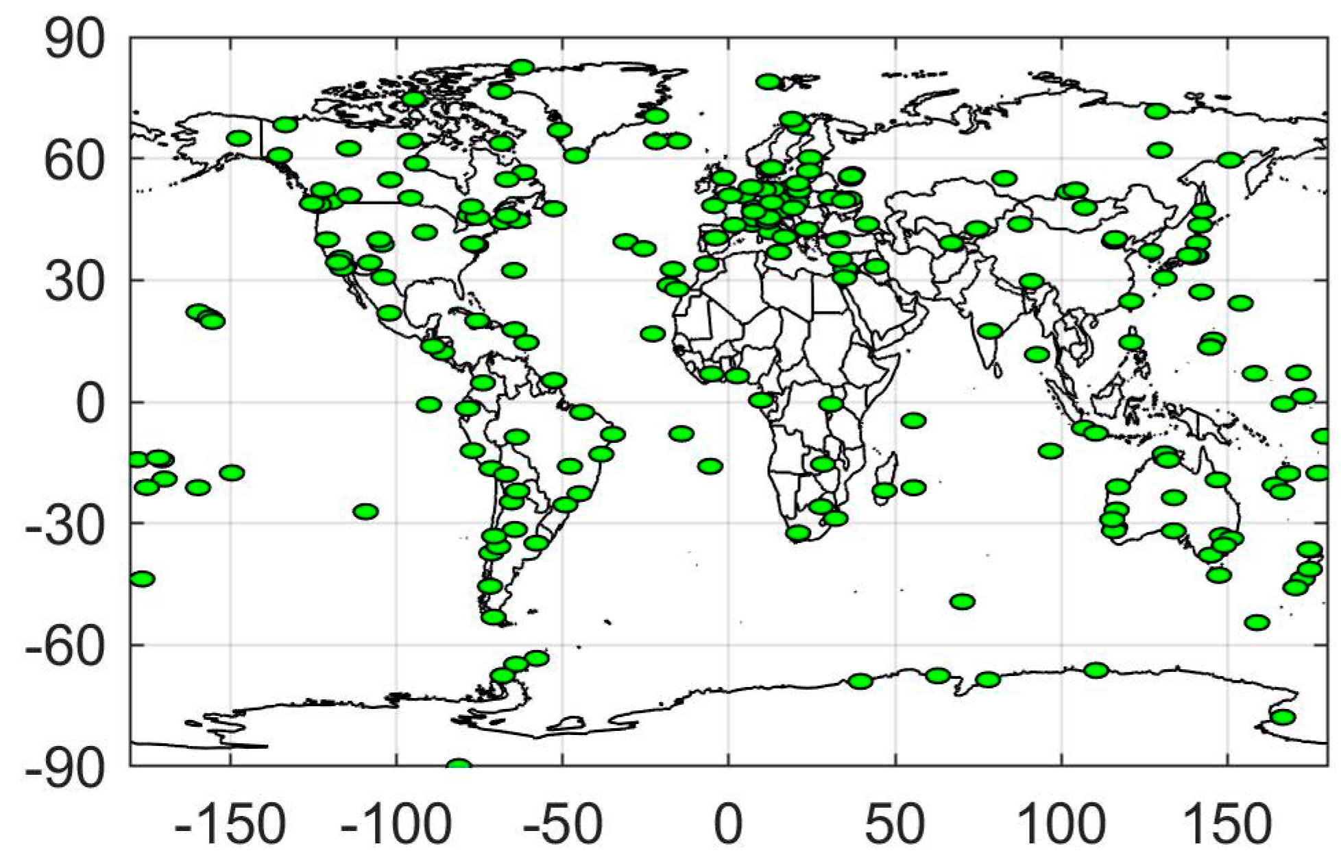
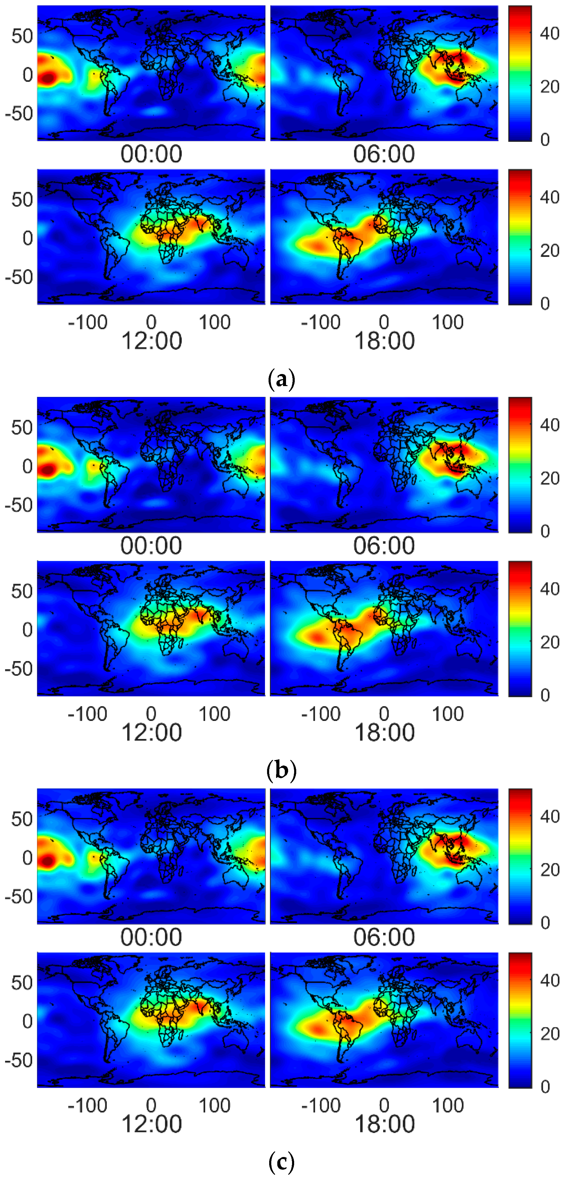
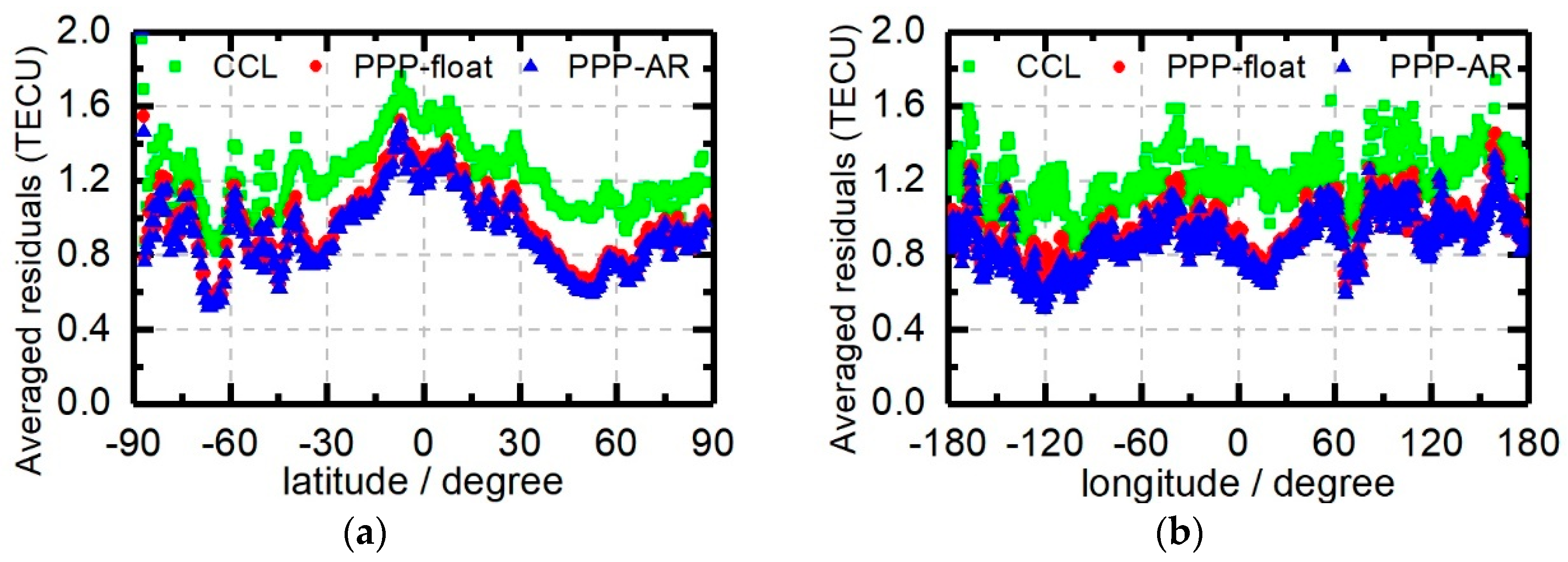
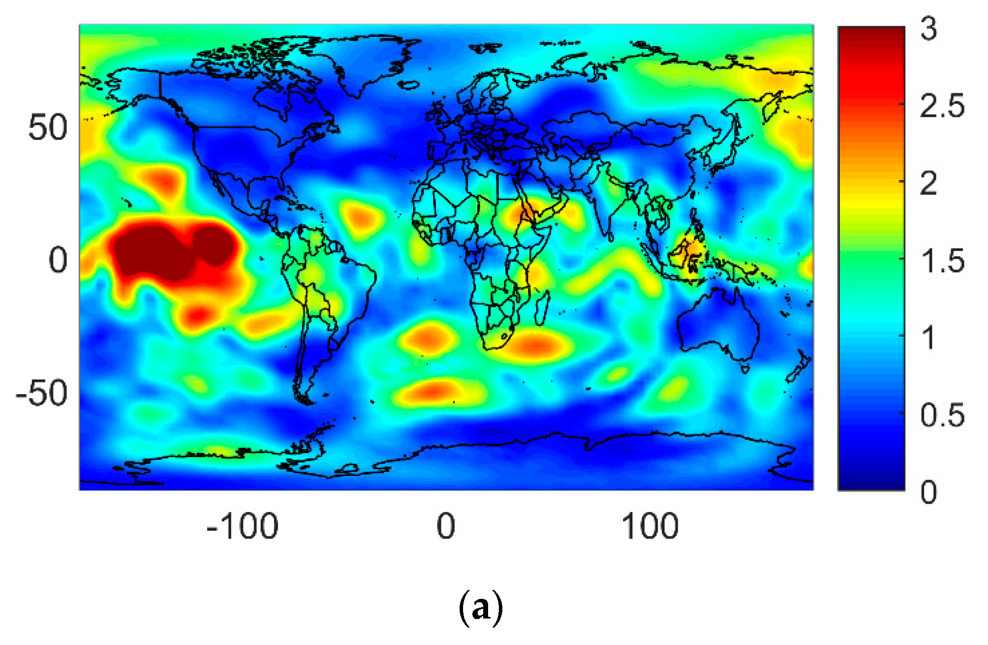
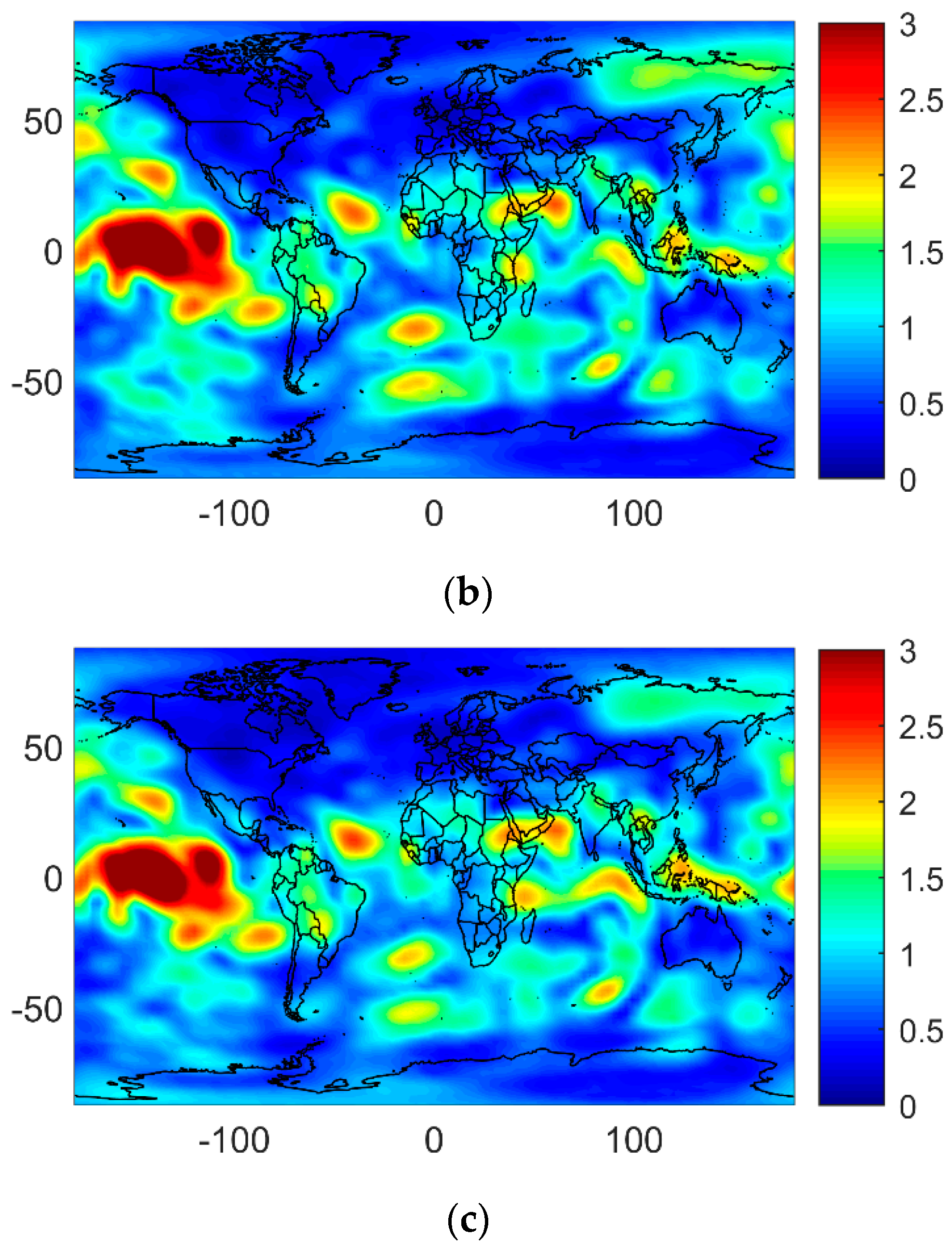
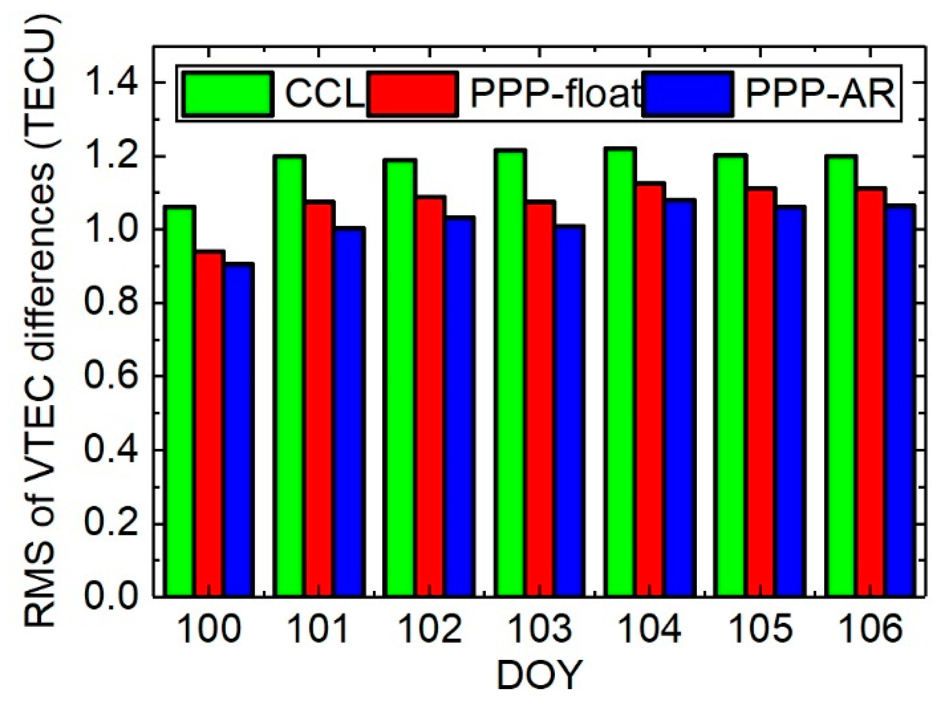
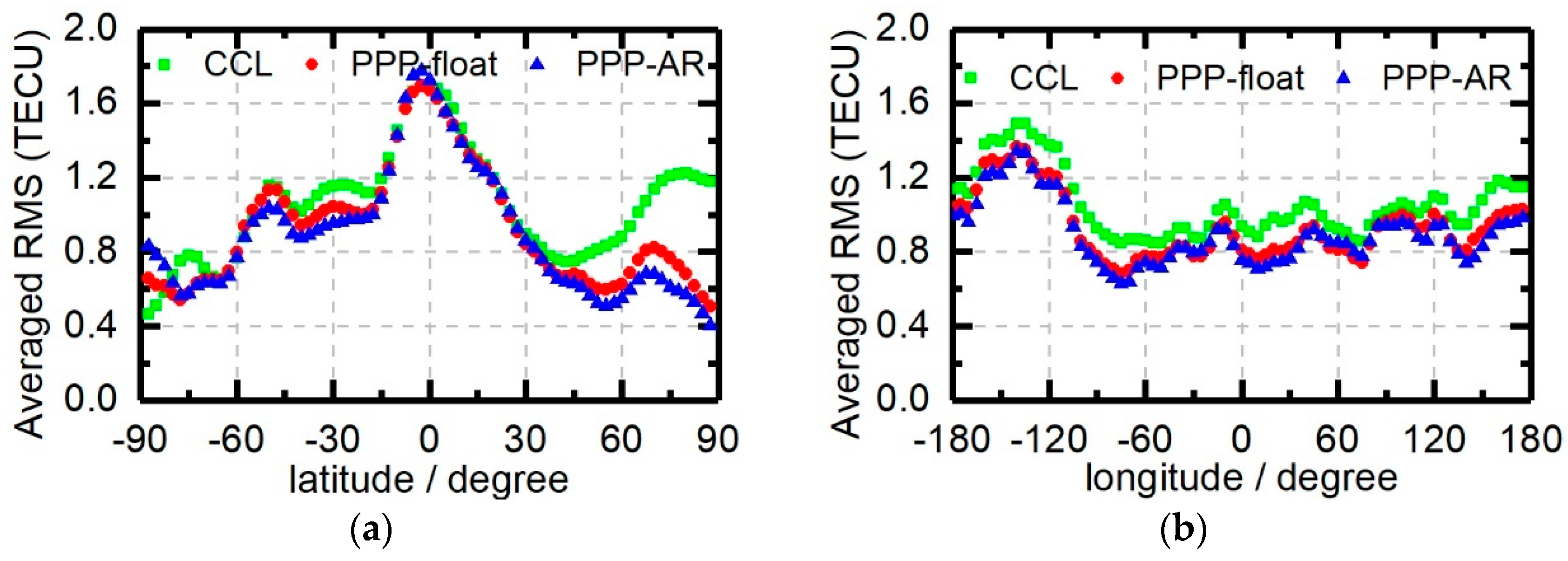
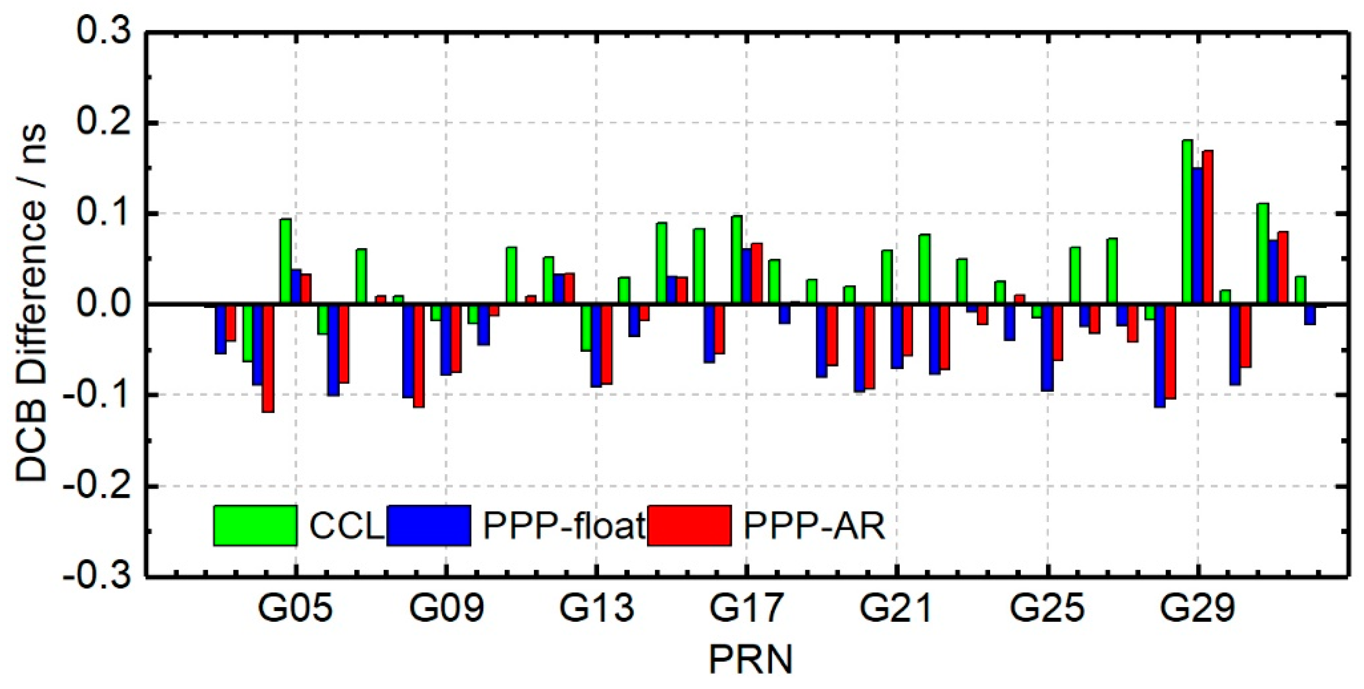
The experiments of ionospheric modeling with different ionospheric observables were processed to compare these with the CODE final GIM products. Consequently, high consistency of the self-generated GIMs products was achieved by the spherical harmonic model with both an order and degree of 15. From the distribution of residuals of ionospheric observables, the IPPs cover mainly areas over the world. However, the absence of stations in oceanic areas can affect the ionosphere modeling. The large residuals, mainly located in low latitude areas, indicate that the active ionosphere with high dynamic temporal and spatial variations degrades the accuracy of ionosphere modeling. This is another limitation that affects the accuracy of the ionospheric map corrections and it was not a focus in this study. Compared with CODE final GIM products, the results prove that the largest differences between self-generated and CODE-generated VTEC products are located in areas where there are no reference stations. A significant improvement was achieved in high latitude areas, especially in the northern hemisphere. As the coproducts of ionosphere modeling, the satellite DCB products were assessed compared with CODE final monthly products. A significant improvement was presented for PPP-AR compared with the PPP-float and CCL solutions. This implies that the fixed undifferenced carrier-phase ambiguities directly improved the estimation performance of ionosphere parameters in the uncombined PPP method.


