Article

Characterizing Forest Dynamics with Landsat-Derived Phenology Curves

by
M. Brooke Rose
1,* and
Nicholas N. Nagle
2
1
Department of Botany and Plant Sciences, University of California, Riverside, CA 92521, USA
2
Department of Geography, University of Tennessee, Knoxville, TN 37916, USA
*
Author to whom correspondence should be addressed.
Remote Sens. 2021, 13(2), 267; https://doi.org/10.3390/rs13020267
Submission received: 10 December 2020 / Revised: 10 January 2021 / Accepted: 11 January 2021 / Published: 14 January 2021
(This article belongs to the Section Forest Remote Sensing)

Abstract

:
Landsat is among the most popular satellites used for forest change assessments. Traditionally, Landsat data users relied on annual or biennial images to measure forest recovery after disturbance, a process that is difficult to monitor at broad scales. With the availability of free Landsat data, intra-annual change analyses are now possible. Phenology, the timing of cyclical vegetation events, can be estimated using indices derived from intra-annual remote sensing data and used to classify different vegetation types after a disturbance. We used a smoothed harmonic modelling approach to estimate NDVI and NBR phenology patterns in pre- and post-fire Landsat sample pixels for two forest groups in South Carolina, using nearby unburned samples as an approximate control group. These methods take advantage of all available images collected by Landsat 5, 7, and 8 for the study area. We found that within burned samples, there were differences in phenology for the two forest groups, while the unburned samples showed no forest group differences. Phenology patterns also differed based on fire severity. These methods take advantage of the freely available Landsat archive and can be used to characterize intra-annual fluctuations in vegetation following a variety of disturbances in the southeastern U.S. and other regions. Our approach builds on other harmonic approaches that use the Landsat archive to detect forest change, such as the Continuous Change Detection and Classification (CCDC) algorithm, and provides a tool to describe post-disturbance forest change.

Graphical Abstract

1. Introduction

One of the most challenging aspects of ecological monitoring over large regions is quantifying and characterizing post-disturbance forest recovery. Forest recovery is a complex process, and forests often have multiple potential successional pathways following a disturbance, depending on disturbance type, pre-disturbance species composition, and landscape topography [1]. Additionally, forest disturbances are infrequent, impacting less than 2% of U.S. forestlands per year from 1985–2005 [2], which limits the data available for forest recovery assessments. However, patterns and rates of post-disturbance forest recovery are key indicators of forest health and resilience [3] and understanding how forests are recovering multiple years following a disturbance is essential for holistic ecological monitoring.
Images collected by earth-orbiting satellites are powerful tools for understanding forest change over time and across various geographic scales. Remote sensing has been extensively used to detect forest disturbance events, including harvest [4], insects [5,6,7], and fire [8]. However, characterizing forest recovery following a disturbance with annual remotely sensed imagery remains challenging. Changes in forest composition after a disturbance are often more complex than can be detected from traditional two-image change detection methods [9]. When assessed annually, common vegetation indices derived from remotely sensed imagery do not always represent ecological definitions of forest recovery [10,11]. Vegetation indices collected from a single image during peak growing season provide only a partial “fingerprint” of the vegetation dynamics occurring on the ground. With an increase in free, moderate-resolution imagery, i.e., Landsat, and the advent of big data processing, we now have access to data collected throughout the year over the span of multiple years, providing a more complete fingerprint that can be used to better understand vegetation dynamics. These results can then be applied to wall-to-wall mapping efforts, which are essential for broad-scale ecological management [12,13].
Intra-annual vegetation patterns, or phenology, vary by vegetation type [14] and can serve as indicators of forest health [15]. A variety of statistical methods have been developed to construct reliable phenology signals from remote sensing data, including Fourier series-based harmonic models [16,17] and logistic regression [18,19]. Phenological metrics derived from these curves have also been used to characterize different vegetation types in non-forested ecosystems [20]. Most of the research on vegetation phenology using remote sensing data has been conducted using coarse spatial resolution data derived from AVHRR and MODIS satellites [18,21,22,23,24]. Recently, research using MODIS-derived land surface phenology suggests that wildfires influence the timing of annual vegetation events, including the start and end of season and maximum greenness [24]. However, with the increasing availability of free Landsat data which are collected at a finer spatial resolution (30 m), researchers are now able to explore the seasonal patterns and intra-annual variability of vegetation across more heterogenous landscapes [19]. As big data processing becomes more feasible, users are now able to take advantage of the full Landsat archive through algorithms such as the Continuous Change Detection and Classification (CCDC) and Breaks for Additive Seasonal Trend (BFAST), which use all available Landsat data for a user-specified location and time period to detect changes in seasonal patterns for a variety of land cover types [25,26]. Access to multiple Landsat observations at multiple times of year has allowed researchers to identify the year-to-year variation in phenology patterns in a broadleaf deciduous forest, demonstrating the ability of Landsat data to capture spatial variability across heterogenous landscapes [19]. Computational resources are now available that allow researchers with modest equipment to use the data-rich Landsat archive to study patterns of intra-annual vegetation dynamics at moderate spatial resolutions.
Our objective was to develop a method capable of constructing Landsat-derived phenology curves which can be used to characterize the seasonal patterns of two forest groups, one primarily evergreen species and the other consisting of primarily deciduous species, undergoing disturbance and recovery. We employ a harmonic regression analysis that has not previously been applied to a Landsat time series for forested landscapes. Harmonic regression uses trigonometric functions to estimate a cyclical time series. Typically, harmonic regression is limited to a few harmonics, such as annual or semi-annual cycles. This limited view of harmonic regression is incapable of capturing nuances in phenology curves, such as different rates of greening and senescence. Borrowing from ideas of spline regression, we employ a penalized harmonic regression that allows us to use many more harmonic components, offering the flexibility to estimate many nuances in the phenology signal while avoiding the problems of overfitting that often arise when using regression with many terms. In this paper we demonstrate this procedure by comparing the average pre- and post-fire intra-annual patterns of two widely-used spectral indices, Normalized Difference Vegetation Index (NDVI) and Normalized Burn Ratio (NBR) using all available Landsat imagery for a forested area in South Carolina, USA collected between 1984–2017. In this analysis, we also compare two distinct forest groups, loblolly-shortleaf pine and oak-gum-cypress, which provide an opportunity to compare phenology patterns between evergreen and deciduous stands, which should vary in their intra-annual spectral signatures.
It is helpful to compare and contrast our approach with the widely used CCDC algorithm [25]. CCDC also uses harmonic regression; however, it is limited to a sinusoidal wave with once-yearly frequency. This annual cycle captures most of the interannual variation represented by the summer–winter difference, but plant phenology is not a simple sinusoidal wave; rather, it is a cyclical pattern [17]. The limited harmonic approach of CCDC creates a stable and reliable predictor of spectral signals, which has proven a powerful device for the automatic detection of forest change. Our motivation is quite different—we are not interested in detecting forest change, but rather in developing tools for describing forest change. Our goal is not to detect change, but to develop the inter-annual phonology pattern as a descriptive statistic of interest, and we develop a flexible harmonic approach that enables a descriptive comparison of phenological cycles before, during and after change.

2. Materials and Methods

2.1. Study Area

The study area selected corresponds to the Landsat scene path 16 row 37 (Figure 1). This region is dominated by the loblolly-shortleaf pine forest group with oak-gum-cypress forests in lower-lying terrain [27]. It falls within the Southeastern Plains and Coastal Plains ecoregions and is characterized by low elevation. This area represents one of the four focal areas in the North American Forest Dynamics (NAFD) project, which aims to better understand forest disturbance and carbon stocks in North American forests [28,29]. Low-severity prescribed fires are common in this region and are implemented to maintain pine-grassland ecosystems, providing ample fire perimeter and severity data that can be used to better understand differences in recovery dynamics between the two dominant forest groups [30].

2.2. Study Data

2.2.1. Landsat Imagery

We used 660 images collected by Landsat Thematic Mapper (TM), Enhanced Thematic Mapper (ETM+) and Operational Land Imager (OLI) for the study area from 1984–2017 (Figure 2). The Landsat Collection 1 Surface Reflectance data were downloaded from the USGS website in November 2017. Landsat TM and ETM+ are atmospherically corrected using the Landsat Ecosystem Disturbance and Adaptive Processing System (LEDAPS) algorithm (version 3.4.0) and Landsat OLI data are produced using the Land Surface Reflectance Code (version 1.4.1) [31,32,33].

2.2.2. Forest Group Maps and Fire Data

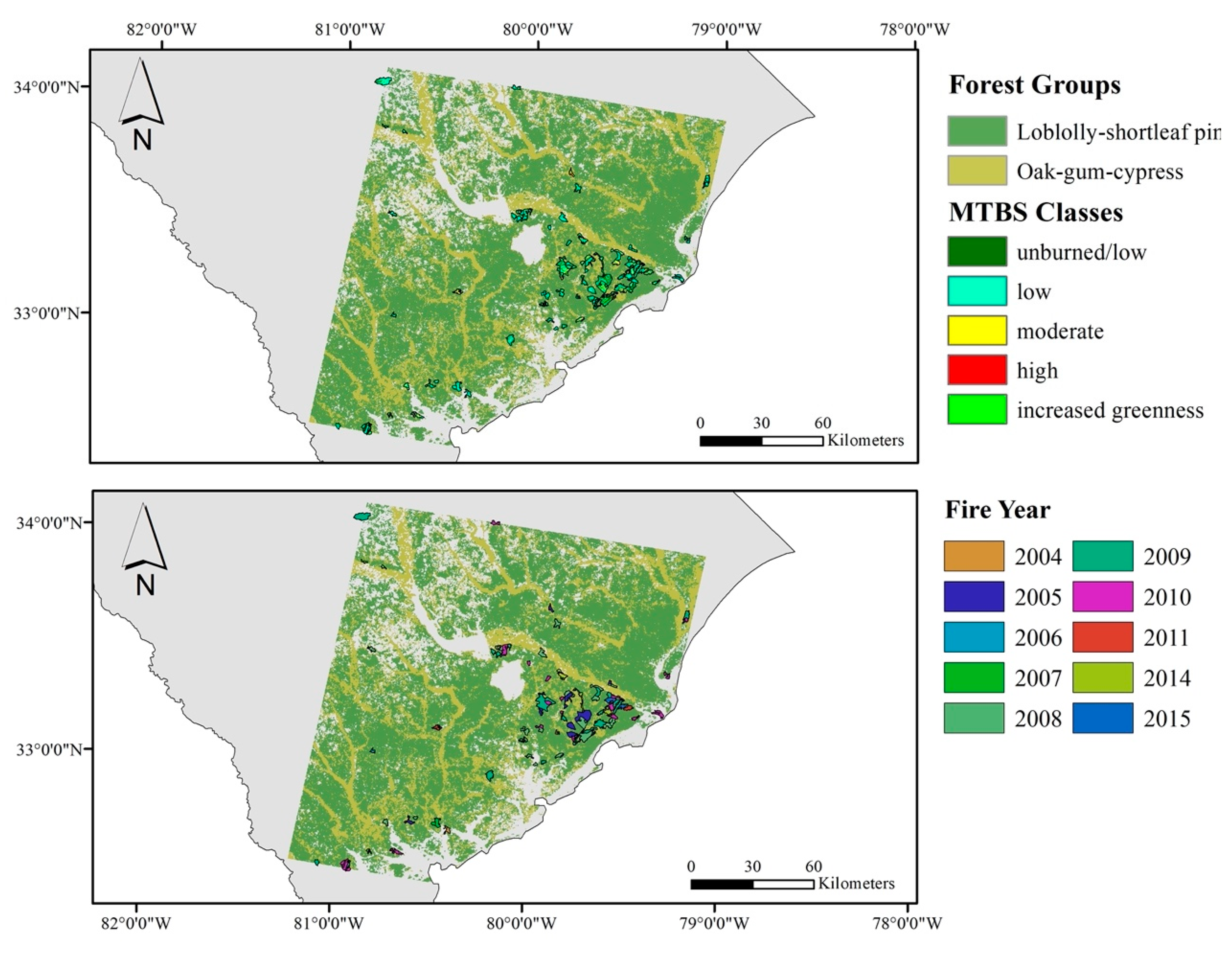
U.S. Forest Service forest group maps were used to distinguish between the two dominant forest species groups in the study area (Figure 3). These maps were derived from a variety of data, including digital elevation models (DEM), Moderate Resolution Spectroradiometer (MODIS) vegetation indices, National Land Cover Dataset (NLCD), and Forest Inventory and Analysis Data and have a spatial resolution of 250 meters [34]. Loblolly-shortleaf pine and oak-gum cypress are two dominant forest groups in the study area.
To distinguish between burned and unburned areas, we used fire extent and severity data produced by the Monitoring Trends in Burn Severity (MTBS) program (Figure 3). These data use Landsat-derived dNBR, the difference between pre- and post-fire NBR, which is a spectral index that combines the near infrared (NIR) and shortwave infrared (SWIR) wavelengths and is often used to identify burned vegetation [35,36]. MTBS data can be downloaded here: https://www.mtbs.gov/direct-download. Because the U.S.F.S. forest group maps were generated in 2003 and past species distribution maps are unavailable, we limited our analysis to fires that occurred between 2003 and 2015 to control for changes in forest group composition that occurred prior to the creation of these maps and to ensure that the forest group maps represent pre-fire conditions.

2.3. Sample Design and Data Processing

We used a pseudo control-treatment sample design, with burned forest locations as the treatment and the surrounding unburned forest locations serving as the control (Figure 4). To better understand the differences between pre- and post-fire phenology within the burned samples, we needed to establish a baseline or “normal” set of phenology curves for forest that did not experience fire. Prior to selecting our burned samples, we removed areas that experienced more than one fire between 1984 and 2015 to reduce any confounding factors introduced by multiple burns. Using the single-burn pixels from the MTBS raster images from 2003–2015, we then sampled 1000 locations from the two forest groups, loblolly-shortleaf pine and oak-gum-cypress, for a total of 2000 burned pixels. For the control pixels, we generated 5-kilometer buffers around each of the MTBS polygons and removed all overlapping burn areas. These buffers represent unburned, control areas of similar environmental conditions to the burned samples within the fires. We sampled an equal number of pixels from the two forest groups within these buffer areas, for a total of 2000 unburned pixels.
We extracted Landsat image values and quality assurance values at the original 4000 sample locations as well as the eight surrounding pixels for phenology smoothing. These data were processed to include fire type, fire severity, forest group, Landsat image date, band number, time since or before fire, and Landsat sensor. Using the Quality Assessment (QA) bands included in Landsat Surface Reflectance product, we excluded pixels affected by instrumental or atmospheric irregularities. This method allowed us to retain all available images for the study region, while also removing cloudy and contaminated data. In total, 3698 of the original 4000 locations were retained after removing cloudy and contaminated data. We then calculated NDVI and NBR from the original Landsat values and then aggregated the data to 90 m spatial resolution using the original pixel and 8 surrounding pixels to reduce noise and retain patch-level NDVI and NBR measures even if one pixel was contaminated or cloudy on a particular date. Because the fire years ranged from 2003–2015, pre-fire Landsat observations range from one day to 31 years before the fire. Similarly, post-fire includes observations collected immediately after the fire up to 13.5 years post-fire. Note that both the burned and unburned samples include pre- and post-fire observations. For the burned samples, pre-fire curves were constructed using all Landsat observations that were collected before the fire, while “post-fire” corresponds to all observations collected after the corresponding fire. Although the unburned samples did not experience fire, they were sampled from the buffer area of a given fire. Each control, unburned sample corresponds to an individual fire and a set of burned, treatment pixels. Therefore, “pre-fire” unburned samples are observations that were taken from the unburned control area before the corresponding fire occurred. Similarly, “post-fire” unburned samples include all clear observations collected after a particular fire occurred.
In the conceptual framework used to model the pre- and post-fire NDVI (and NBR) phenology curves, S p r e ( t , d a t e t ) is the smooth phenology curve before the fire, which is a function of time and day of the year, S p o s t p r e ( t , d a t e t ) is the change in the phenology curve after the fire, and I() is an indicator variable equal to 0 before fire and 1 for after fire. When predicting the pre-fire seasonal patterns of NDVI and NBR, I = 0 and time after fire is null. This allows us to measure the change in phenology curve pre- and post-fire.
NDVI ^ = S p r e ( t , d a t e t ) + I ( t   a f t e r   f i r e ) S p o s t p r e ( t , d a t e t )

2.4. Harmonic Regression

To model the annual curves of NDVI and NBR derived from Landsat 5 TM, Landsat 7 ETM+, and Landsat 8 OLI pixel samples, we used a non-classical harmonic regression analysis that was developed to construct phenology curves for different land cover types in the Great Basin using AVHRR data [16,17]. Equation (2) gives the formula for a harmonic function with a polynomial trend, where y ^ i represents the predicted NDVI value, and a, b, and c are coefficients to be estimated.
y ^ i = m = 0 L c m t i m + k = 1 M   ( a k c o s ( 2 π k T t i ) + b k s i n ( 2 π k T t i ) )
The coefficient c m captures the intercept and any linear, quadratic, and polynomial time trends.
The coefficients a k and b k capture the annual phenology variation at specific frequencies. The overall curve can be made arbitrarily flexible by making M—the number of sinusoidal terms—very large. Unfortunately, setting M to be large also tends toward overfitting. We modified the harmonic regression by using penalized least squares, which is a technique used in smoothing spline methods, which penalizes the magnitude of the coefficients a k and b k [37] and ameliorating overfitting. The practical effect of this penalization is that it allows us to include many harmonic components, allowing us to flexibly estimate phenology curves while avoiding overfitting and spurious harmonic terms.
The formulas for the penalized least squared method are:
m i n i ( y i y i ^ ) 2 +   λ   × w i g g l i n e s s
w i g g l i n e s s =   k = 1 M ( a k 2 +   b k 2 )
The penalized least squares will choose the coefficients a, b and c to best fit the data, but the harmonic terms a and b are added with a penalty to avoid “wiggliness”. The parameter λ controls the tradeoff between fit and wiggliness, and its effect is explored below.
Landsat scenes are imaged by the OLI, TM, or ETM+ sensor every sixteen days, making time-sensitive phenology assessments from Landsat more challenging than other sensors with high-temporal resolution, e.g., AVHRR or MODIS. In contrast to those data, however, Landsat data are collected at a 30 m spatial resolution, allowing for more precise characterization of heterogenous landscapes than is possible using AVHRR or MODIS. Harmonic regression analysis using Landsat 5 TM and Landsat 7 ETM+ data has been applied to crop phenology research [38]; however, little work has been done to assess the usefulness of this approach in characterizing forest communities and their recovery following a disturbance using Landsat imagery.
Using the harmonic regression modelling approach, we constructed phenological models for different subsets of the Landsat data, based on forest group, burn severity, and time since fire. In constructing the initial models, we prioritized flexibility by allowing for 20 sine and 20 cosine waves every 365 days. Whereas a harmonic regression with 20 terms would normally overfit the data, the penalized regression method allows them to flexibly describe the phenology trend without introducing spurious cycles. These parameters can be adjusted for different data types or ecological systems. The traditional harmonic regression for annual NDVI is too flexible and exhibits overfitting; while it captures fluctuations in NDVI throughout the year it is also quite noisy and does not accurately reflect the average phenology of the forests in the region (Figure 5).
The smoothed harmonic regression model outputs for both forest groups are representative of the expected vegetation green-up phenology in the region, showing a broad summer peak greenness corresponding to the humid subtropical climate of the study area (Figure 6a). It is important to note that the smoothing parameters must be appropriately based on expert knowledge of phenology curves; applying too much smoothing generates curves that provide little information about the seasonal patterns of the land surface being studied, also shown in Figure 6b.

2.5. Phenology Metrics

In addition to constructing phenology curves using a smoothed harmonic regression approach, we derived several phenology metrics from the curves to compare the seasonal differences between the forest groups, pre- and post-fire, and different levels of fire severity. These metrics include the minimum and maximum predicted annual values of NBR and NDVI, the DOY on which the minimum and maximum values occur, and the timing of spring and fall senescence based on NDVI or NBR. There is no universally accepted method for defining or deriving phenology metrics, such as start of spring [22]. However, we selected a method in which a spectral index threshold value (SIratio) is used to identify the spring green up and start of growing season [39]. White et al. [39] used 50% threshold values to identify spring and onset and cessation, a value that works well with a variety of land cover types. In this method, SIratio is the percentage of the seasonal amplitude reached at a given point in time:
S I r a t i o =   S I S I m i n S I m a x S I m i n
To identify the DOY for spring onset and fall senescence from the phenology curves developed in this research, we used 50% threshold values. All data were processed and analyzed using R statistical software, specifically the ‘tidyverse’, ‘sf’, ‘mgcv’ and ‘raster’ packages. The penalized regression was performed using the ‘pcls’function in the ‘mgcv’ package [37]. We have also calculated confidence intervals for all phenology curves intervals are tight and do not change the interpretation of the figures, so we have not reproduced them here.

3. Results

3.1. Fire Summary Statistics

In total, we compared NDVI and NBR Landsat phenology curves in 85 fires and their unburned 5-km buffer areas. The first fire occurred on 8 April 2004 and the last on 30 May 2015. The vast majority of the fires were prescribed (72 fires, 84.7%), followed by wildfires (7 fires, 8.2%), and unknown (6 fires, 7%).
Because fire severity is a pixel-level, categorical variable within the MTBS raster dataset, we used the mode MTBS classification of the samples collected from each fire to roughly estimate severity at the fire-level. The vast majority (91.8%) of the sample fires were unburned/low severity or low severity (mode severity of 1 or 2), with four fires having a mode of moderate severity, one fire showing overall increased greenness and two having predominantly no data/not mapped pixel values (Table 1).
Seasonality is a key component for inferring phenological patterns. Spring was defined as 1 March to 31 May, summer as 1 June to 31 August, autumn/fall as 1 September to 30 November, and winter as 1 December through 28 February. In terms of the seasonal distribution of the fires, the majority occurred in the spring (73%), followed by the winter months (26%), and autumn (<1%). None of the sample fires occurred during the summer months.

3.2. Forest Group Differences

Using the global, penalized harmonic regression model, we constructed phenology curves for the two forest groups in the pre-fire burned and unburned samples (Figure 6, left). The baseline phenology curve of oak-gum cypress shows a greater intra-annual amplitude (i.e., difference between minimum and maximum NDVI) than the baseline curve for loblolly-shortleaf pine. In terms of annual phenology metrics, NDVI in loblolly-shortleaf pine ranged from 0.4969 to 0.7751, with a seasonal amplitude of 0.2480 (Table 2). NDVI predictions in oak-gum-cypress ranged from 0.4702 to 0.7386, with a seasonal amplitude of 0.2683. For the DOY derived from the phenology curves of the two forest groups, DOY of maximum NDVI showed almost no difference, with loblolly-shortleaf pine reaching maximum NDVI at day 248 (4 or 5 September), and oak-gum-cypress reaching maximum NDVI much earlier at day 247 (3 or 4 September).

3.3. Pre- and Post-Fire

For both loblolly-shortleaf pine and oak-gum-cypress, there was little difference in the NDVI phenology patterns between pre- and post-fire (Figure 7). The loblolly-shortleaf pine post-fire predictions do show slightly elevated post-fire NDVI in the late fall and winter, while the oak-gum-cypress post-fire NDVI is lower than pre-fire levels in the summer. The NDVI phenology metrics did not change substantially for either loblolly-shortleaf pine or oak-gum-cypress after fire (Table 3). However, the DOY for maximum NDVI in post-fire oak-gum-cypress was much later in the year (day 247) than for pre-fire oak-gum-cypress (day 191) for the burned samples.
Post-fire NBR for loblolly-shortleaf pine and oak-gum-cypress showed a consistent decrease throughout the year, with the greatest difference occurring from April to October (Figure 7). Post-fire NBR maximum and minimum were lower in both loblolly-shortleaf pine and oak-gum-cypress (Table 4).

3.4. Fire Severity and Time Since Fire

We compared phenology curves between differing levels of fire severity, derived from the MTBS dataset, for each forest group. Post-fire phenology in unburned/low severity forests showed increases in NDVI and NBR throughout the year (Figure 8). The patterns were similar for both forest groups. For low severity fires, post-fire NDVI phenology showed small increases while NBR curves decreased considerably following fire, with the greatest decrease in the summer. Finally, NDVI levels decreased slightly after moderate severity fires, and NBR showed greater decreases, particularly in early spring and summer.
In addition to fire severity, we also modeled phenology curves for two different time steps following fire, within two years post-fire and more than two years post fire (Figure 9). Our results varied depending on spectral index. While loblolly-shortleaf pine had slight decreases in the spring and early summer within two years post-fire, NDVI levels recovered to pre-fire values more than two years after fire. For oak-gum cypress, the decrease observed less than two years after fire was greater than the change observed for loblolly-shortleaf pine. However, NDVI levels more than two years following fire were greater than pre-fire levels. Again, phenology curves for NBR showed different results, with a greater decrease in the spring and summer within two years of fire for both forest groups. In contrast to the NDVI levels, which appeared to recover more than two years after fire, NBR levels remained below pre-fire values, particularly in the late summer and early winter. Phenometrics for time-since-fire show that maximum NDVI and NBR are greater when compared to values more than two years after fire for loblolly-shortleaf pine (Table 5 and Table 6). However, the opposite was true in oak-gum-cypress plots, with maximum NDVI and NBR reaching higher levels more than two years after fire. The timing of these maximum values also shifts depending on time since fire, with maximum NDVI and NBR occurring later in the year for both forest groups in the two years immediately after fire when compared to more than two years post-fire.

3.5. Comparing Burned and Unburned Samples

Phenology curves constructed from the unburned samples revealed no differences between loblolly-shortleaf pine and oak-gum-cypress (Figure 9). The NDVI phenology metrics for the unburned samples revealed no differences between forest groups (Table 5). Phenology curves in the unburned samples showed distinct increases in NDVI post-fire when compared to pre-fire curves for both forest groups throughout the year (Figure 10). There were only small changes in the NBR phenology curves for pre- and post-fire samples in the control group (Figure 10). Note that the “pre-fire” and “post-fire” designations refer to when the corresponding burned samples experienced fire. Post-fire NDVI phenology curves for loblolly-shortleaf pine and oak-gum-cypress showed an increase in both minimum and maximum NDVI, with no distinct changes in the DOY on which these events occurred (Table 7). The seasonal amplitude for NDVI and NBR phenology increased in post-fire loblolly-shortleaf pine and oak-gum-cypress (Table 7 and Table 8).

4. Discussion

4.1. Forest Group Differences

The phenology models for oak-gum-cypress curve had a greater seasonal amplitude than the loblolly-shortleaf pine model. These results support previous findings that phenology is a useful remotely sensed metric for distinguishing between different vegetation classifications, particularly between deciduous and evergreen forest types [13]. However, the loblolly-shortleaf pine model demonstrated more seasonality than expected for an evergreen forest group, likely due to the heterogeneity of the forest cover in this region with broadleaf deciduous plants found in lower strata.
One potential issue with these findings is that the original forest group map classifications were developed in 2003 and were assumed to remain constant throughout the study period. In the future, post-fire metrics collected in the field could be related to phenology curves over time for a more dynamic understanding of forest group composition change. While the forest group phenology curves constructed from the pre-fire sample data revealed some differences, the curves constructed from the unburned samples did not differ by forest group. The discrepancies between the forest group differences found in the burned samples vs. the unburned samples is addressed later in the discussion.

4.2. Pre- and Post-Fire

Pre- and post-fire phenology differences were dependent on the spectral index chosen for analysis. In the original pre- and post-fire phenology models, both loblolly-shortleaf pine and oak-gum-cypress demonstrated almost no change in NDVI. However, NBR, which takes advantage of the ratio between the near-infrared and shortwave infrared values, is commonly used to identify and assess burned vegetation, decreased from pre- to post-fire. Both of these indices have been used to measure the difference between pre- and post-fire vegetation [40], and recent research suggests that NDVI levels return to pre-fire levels in a shorter time frame than observed for NBR [41]. This finding provides a potential explanation for the relatively small difference in pre- and post-fire NDVI. In our study area, the fire regime consists of mainly low severity ground fires that do not affect the tree stratum and canopy-level greenness, which is measured by NDVI. The larger differences in NBR, even averaged across multiple years following fire, could indicated that it is a more informative spectral index for measuring long-term recovery patterns in areas with low-severity fires. In contrast, the adjacent unburned samples showed increased NDVI values post-fire when compared to pre-fire levels.

4.3. Fire Severity and Time Since Fire

Post-fire phenology patterns differed depending on fire severity. Most of the study fires were low in severity, with mode pixel severity rankings of 1 or 2 (unburned/low severity and low severity fires). For unburned/low severity fires, both forest groups demonstrated an increase or no change in NDVI after fire. NDVI phenology following moderate fires showed only small decreases. However, NBR decreased throughout the year for all levels of fire severity, with the greatest decrease after moderate severity fires. In our analysis of time since fire, we observed that NDVI levels returned to or exceeded pre-fire levels for both forest groups given more than two years post-fire (Figure 9). However, NBR levels remained lower than pre-fire levels even more than two years post-fire, particularly in the late summer and winter months. These findings align with our earlier discussion of the differences between NBR and NDVI and further suggests that NBR may be more suitable for assessing forest recovery after fire in areas with generally prescribed, low severity fires that do not influence canopy greenness in the long term.

4.4. Differences between the Burned and Unburned Samples

Among the most surprising findings of this research were the results of the burned to unburned sample comparisons. While the phenology curves and metrics derived from the burned samples showed differences between loblolly-shortleaf pine and oak-gum-cypress, there were essentially no forest group differences in the unburned samples (Figure 9). While pre- and post-fire NDVI phenology in the burned samples showed very small differences, the unburned samples showed a distinct upward shift in NDVI during the time period after the corresponding burned sites experienced fire. NBR phenology curves were more representative of the expected results, with a downward shift from pre- to post-fire in burned samples and no change between pre- and post-fire phenology in the corresponding unburned samples. Because most of the fires carried out in the study area are prescribed and not wildfire, it is possible that the unburned samples are not as environmentally similar to the burned samples as assumed in the research design.
There are some potential ecological explanations for the similar phenological patterns observed for unburned loblolly-shortleaf pine and oak-gum-cypress. One of the primary goals of prescribed burning in the Coastal Plains ecosystem is to maintain pine-grassland forest types [42]. Because the phenology curves and metrics for the unburned loblolly-shortleaf pine more closely matched the seasonal patterns of a deciduous forest, it is possible that in the absence of fire for the study period, these pine-grasslands have not been maintained in the unburned samples, leading to loblolly-shortleaf pine transitioning to deciduous forest. This observation is supported by research on the widespread transition from fire-tolerant pine to fire-intolerant hardwood species in the southeastern U.S. under fire suppression [43]. Nevertheless, more analysis is needed to confirm these patterns.

4.5. Future Considerations

We have developed baseline phenology curves in forest areas for loblolly-shortleaf pine and oak-gum-cypress before and after varying levels of fire severity using all Landsat OLI, ETM+, and TM images collected between 1984–2017 for our study area in South Carolina. However, future work is needed to test and validate the phenology curves for vegetation discrimination and classification. Research that requires a formal statistical test of phenology difference can be accomplished by fitting the model with and without the interaction terms and comparing them with an AIC or F statistic. For our analysis, we selected smoothing parameters based on the seasonal nature of phenology and our expectations for the seasonal patterns in the study area. We chose the smoothing based on visual comparison of the empirical phenology curve (Figure 6) with our well-informed knowledge of phenology curves—a more data-driven approach might be to choose the smoothing parameter with some form of k-fold validation.
In this study, we removed areas that burned multiple times over the course of the study period. However, the management practices implemented in the loblolly-shortleaf pine forests of South Carolina includes repeat burning. Therefore, a potential future study could compare the recovery characteristics in forests that are burned multiple times over the course of a few decades to those that are only burned once. A key management goal in forest management areas like Francis Marion National Forest is to maintain or, in some cases, reintroduce the pine-grassland ecosystems native to the region, which requires frequent, low-intensity burning [30,42]. Understanding how these prescribed burns affect vegetation composition is essential to making informed management decisions.
The goal of this research was to move towards developing methods that could be applied to a large region or regions to characterize forest recovery after a variety of disturbances, not just fire. Though this paper only examined patterns related to fire disturbance, forests in this region are also subject to timber harvesting [44], hurricane disturbance [45], and insect defoliation via southern pine beetle infestations [46], and these areas were not excluded from our analysis. Though this is a limitation of the current study, future research could examine the impacts of harvest, insects, disease, and hurricanes on the phenological signatures of vegetation. We also acknowledge that some regions experience greater cloud cover, shorter vegetation growing seasons, and have less available imagery. Future research should examine the minimum number of images or clear pixels necessary to characterize a specific landscape. However, combining data from multiple remote sensing platforms, such as Sentinel 2 and Landsat 8, can vastly increase data frequency for time series analysis [47] and could facilitate phenology research in areas with fewer clear images than our study area. We also note that there are small but potentially significant differences between Landsat 8 and the older Landsat 5 and 7 data and that future research could correct for these differences, depending on the user’s application [48]. In this study, we used Landsat data to produce baseline annual phenology curves for two forest groups before and after fire. Unlike methods that generate multiple annual timeseries, such as the Continuous Change Detection and Classification algorithm, our method is not designed to detect disturbances. However, our results support using Landsat-derived phenology estimates to characterize forest recovery following fire and could be applied to better understand forest recovery following a variety of disturbances.

5. Conclusions

Detecting forest change from space requires the comparison of spectral signals over time. Classical techniques have relied on the comparison of a few images. Spectral signals can change in many ways, for example the timing and slope of greenup and senescence can change or the timing of the peak NDVI can shift. Landscape change can display in the spectral signature as a changing phenological curve, and not just a change in levels represented by a small selection of images.
In this paper, we have presented a simple curve-fitting method that captures these phenological changes using the entire Landsat image stack, rather than just few images. Since phenology is seasonal, we have use curve-fitting based on harmonic regression. All curve-fitting methods can suffer from overfitting, and previous effort at harmonic fitting have addressed this be including just a few low frequency components. These are a good start, but they do not represent phenology well because plant phenology is not a precise sinusoidal wave. We used the statistical technique of penalized regression to more flexibly fit a curve to the image stack while avoiding overfitting. Our method relies on well-established packages from the R statistical software and is accessible from current desktop computers. These methods could also be implemented using Google Earth Engine, which does not require the user to download all Landsat images for analysis and has been used for harmonic modeling with remote sensing data [6,49].
Our results demonstrated that Landsat NDVI and NBR phenology curves in loblolly-shortleaf pine differed from the phenology curves of oak-gum-cypress. As expected, post-fire NBR phenology curves in both forest groups showed a decrease from pre-fire levels, with some variability in the magnitude of that decrease throughout the year. There was no difference between the forest group phenology curves of the unburned samples. While additional analysis is necessary to understand the differences observed between phenology patterns of the burned and unburned samples, a potential ecological explanation for this pattern could be that the lack of fire for the study period has led to the homogenization of forest groups, with the loblolly-shortleaf pine transitioning into a deciduous forest type. Although more work is needed to refine the uncertainty measures of these phenology curves, the current results suggest that deriving phenology curves from Landsat data is a feasible approach for better understanding forest recovery after fire.
These findings provide information about successional patterns and differences between forest groups following fire, which are key components of forest health and aid in forest management decisions. Phenology metrics and patterns derived from remote sensing imagery with relatively fine temporal yet coarse spatial resolution (i.e., MODIS and AVHRR) have been used to characterize patterns in disturbance and recovery cycles across broad spatial scales. However, forest disturbance-recovery dynamics are often spatially heterogenous, with important changes occurring across gradients at finer spatial scales than can be detected by these sensors. The methods we present allow researchers to more reliably monitor forest dynamics at finer spatial resolutions than has been traditionally feasible. Using the entire Landsat stack, scientists can develop richer and more sensitive measures of change. These measurements will contribute to the improvement of continuous sensing of forest landscapes.

Author Contributions

Conceptualization, M.B.R. and N.N.N.; methodology, M.B.R. and N.N.N.; writing—original draft preparation, M.B.R.; writing—review and editing, M.B.R. and N.N.N.; funding acquisition, N.N.N. All authors have read and agreed to the published version of the manuscript.

Funding

This research received no external funding.

Institutional Review Board Statement

Not applicable.

Informed Consent Statement

Not applicable.

Data Availability Statement

The data presented in this study are openly available in Zenodo at http://doi.org/10.5281/zenodo.4019600.

Acknowledgments

The authors would like to thank Janet Franklin, Sally Horn, Monica Papeş, and three anonymous reviewers for their valuable comments and suggestions, which greatly improved previous versions of the manuscript. MTBS data were obtained from www.mtbs.gov; U.S.F.S. forest group maps were obtained from https://data.fs.usda.gov/geodata/rastergateway/forest_type/conus_forest_type_group_metadata.php.

Conflicts of Interest

The authors declare no conflict of interest.

References

  1. Swanson, M.E.; Franklin, J.F.; Beschta, R.L.; Crisafulli, C.M.; DellaSala, D.A.; Hutto, R.L.; Lindenmayer, D.B.; Swanson, F.J. The forgotten stage of forest succession: Early-successional ecosystems on forest sites. Front. Ecol. Environ. 2011, 9, 117–125. [Google Scholar] [CrossRef] [Green Version]
  2. Masek, J.G.; Goward, S.N.; Kennedy, R.E.; Cohen, W.B.; Moisen, G.G.; Schleeweis, K.; Huang, C. United States Forest Disturbance Trends Observed Using Landsat Time Series. Ecosystems 2013, 16, 1087–1104. [Google Scholar] [CrossRef] [Green Version]
  3. Lebrija-Trejos, E.; Bongers, F.; Pérez-García, E.A.; Jorge, A.M. Successional Change and Resilience of a Very Dry Tropical Deciduous Forest Following Shfiting Agriuclture. Biotropica 2008, 40, 422–431. [Google Scholar] [CrossRef]
  4. Cohen, W.B.; Spies, T.A.; Alig, R.J.; Oetter, D.R.; Maiersperger, T.K.; Fiorella, M. Characterizing 23 years (1972–1995) of stand replacement disturbance in western Oregon forests with landsat imagery. Ecosystems 2002, 5, 122–137. [Google Scholar] [CrossRef]
  5. Senf, C.; Pflugmacher, D.; Wulder, M.A.; Hostert, P. Characterizing spectral-temporal patterns of defoliator and bark beetle disturbances using Landsat time series. Remote Sens. Environ. 2015, 170, 166–177. [Google Scholar] [CrossRef]
  6. Housman, I.W.; Chastain, R.A.; Finco, M.V. An evaluation of forest health insect and disease survey data and satellite-based remote sensing forest change detection methods: Case studies in the United States. Remote Sens. 2018, 10, 1184. [Google Scholar] [CrossRef] [Green Version]
  7. Pasquarella, V.J.; Bradley, B.A.; Woodcock, C.E. Near-real-time monitoring of insect defoliation using Landsat time series. Forests 2017, 8, 275. [Google Scholar] [CrossRef] [Green Version]
  8. Lentile, L.B.; Holden, Z.A.; Smith, A.M.S.; Falkowski, M.J.; Hudak, A.T.; Morgan, P.; Lewis, S.A.; Gessler, P.E.; Benson, N.C. Remote sensing techniques to assess active fire characteristics and post fire effects. USDA For. Serv. UNL Fac. Publ. 2006, 194, 319–345. [Google Scholar] [CrossRef]
  9. Rogan, J.; Franklin, J.; Roberts, D.A. A comparison of methods for monitoring multitemporal vegetation change using thematic mapper imagery. Remote Sens. Environ. 2002. [Google Scholar] [CrossRef]
  10. Huang, C.; Goward, S.N.; Masek, J.G.; Thomas, N.; Zhu, Z.; Vogelmann, J.E. An automated approach for reconstructing recent forest disturbance history using dense Landsat time series stacks. Remote Sens. Environ. 2010, 114, 183–198. [Google Scholar] [CrossRef]
  11. Buma, B. Evaluating the utility and seasonality of NDVI values for assessing post-disturbance recovery in a subalpine forest. Environ. Monit. Assess. 2012, 184, 3849–3860. [Google Scholar] [CrossRef] [PubMed]
  12. Kerr, J.T.; Ostrovsky, M. From space to species: Ecological applications for remote sensing. Trends Ecol. Evol. 2003, 18, 299–305. [Google Scholar] [CrossRef]
  13. Pasquarella, V.J.; Holden, C.E.; Woodcock, C.E. Improved mapping of forest type using spectral-temporal Landsat features. Remote Sens. Environ. 2018, 210, 193–207. [Google Scholar] [CrossRef]
  14. Piao, S.; Fang, J.; Zhou, L.; Ciais, P.; Zhu, B. Variations in satellite-derived phenology in China’s temperate vegetation. Glob. Chang. Biol. 2006, 12, 672–685. [Google Scholar] [CrossRef]
  15. Lambert, J.; Drenou, C.; Denux, J.P.; Balent, G.; Cheret, V. Monitoring forest decline through remote sensing time series analysis. GIScience Remote Sens. 2013, 50, 437–457. [Google Scholar] [CrossRef]
  16. Bradley, B.A.; Jacob, R.W.; Hermance, J.F.; Mustard, J.F. A curve fitting procedure to derive inter-annual phenologies from time series of noisy satellite NDVI data. Remote Sens. Environ. 2007, 106, 137–145. [Google Scholar] [CrossRef]
  17. Hermance, J.F. Stabilizing high-order, non-classical harmonic analysis of NDVI data for average annual models by damping model roughness. Int. J. Remote Sens. 2007, 28, 2801–2819. [Google Scholar] [CrossRef]
  18. Zhang, X.; Friedl, M.A.; Schaaf, C.B.; Strahler, A.H.; Hodges, J.C.F.; Gao, F.; Reed, B.C.; Huete, A. Monitoring vegetation phenology using MODIS. Remote Sens. Environ. 2003, 84, 471–475. [Google Scholar] [CrossRef]
  19. Melaas, E.K.; Friedl, M.A.; Zhu, Z. Detecting interannual variation in deciduous broadleaf forest phenology using Landsat TM/ETM+ data. Remote Sens. Environ. 2013, 132, 176–185. [Google Scholar] [CrossRef]
  20. Van Leeuwen, W.J.D.; Davison, J.E.; Casady, G.M.; Marsh, S.E. Phenological characterization of desert sky island vegetation communities with remotely sensed and climate time series data. Remote Sens. 2010, 2, 388–415. [Google Scholar] [CrossRef] [Green Version]
  21. Hwang, T.; Song, C.; Vose, J.M.; Band, L.E. Topography-mediated controls on local vegetation phenology estimated from MODIS vegetation index. Landsc. Ecol. 2011, 26, 541–556. [Google Scholar] [CrossRef]
  22. White, M.A.; de Beurs, K.M.; Didan, K.; Inouye, D.W.; Richardson, A.D.; Jensen, O.P.; O’Keefe, J.; Zhang, G.; Nemani, R.R.; van Leeuwen, W.J.D.; et al. Intercomparison, interpretation, and assessment of spring phenology in North America estimated from remote sensing for 1982–2006. Glob. Chang. Biol. 2009, 15, 2335–2359. [Google Scholar] [CrossRef]
  23. Jönsson, P.; Eklundh, L. Seasonality extraction by function fitting to time-series of satellite sensor data. IEEE Trans. Geosci. Remote Sens. 2002, 40, 1824–1832. [Google Scholar] [CrossRef]
  24. Wang, J.; Zhang, X. Investigation of wildfire impacts on land surface phenology from MODIS time series in the western US forests. ISPRS J. Photogramm. Remote Sens. 2020, 159, 281–295. [Google Scholar] [CrossRef]
  25. Zhu, Z.; Woodcock, C.E. Continuous change detection and classification of land cover using all available Landsat data. Remote Sens. Environ. 2014, 144, 152–171. [Google Scholar] [CrossRef] [Green Version]
  26. Verbesselt, J.; Hyndman, R.; Newnham, G.; Culvenor, D. Detecting trend and seasonal changes in satellite image time series. Remote Sens. Environ. 2010, 114, 106–115. [Google Scholar] [CrossRef]
  27. Barbour, M.G.; Billings, W.D. North American Terrestrial Vegetation, 2nd ed.; Cambridge University Press: Cambridge, UK, 2000. [Google Scholar] [CrossRef]
  28. Goward, S.N.; Masek, J.G.; Cohen, W.; Moisen, G.; Collatz, G.J.; Healey, S.; Houghton, R.A.; Huang, C.; Kennedy, R.; Law, B.; et al. Forest Disturbance and North American Carbon Flux. Earth Obs. Syst. 2008, 89, 28–31. [Google Scholar] [CrossRef]
  29. Huang, C.; Goward, S.N.; Masek, J.G.; Gao, F.; Vermote, E.F.; Thomas, N.; Schleeweis, K.; Kennedy, R.E.; Zhu, Z.; Eidenshink, J.C.; et al. Development of time series stacks of landsat images for reconstructing forest disturbance history. Int. J. Digit. Earth 2009, 2, 195–218. [Google Scholar] [CrossRef]
  30. Fairchilds, L.; Trettin, C. History and Legacy of Fire Effects in the South Carolina Piedmont and Costal Regions; General Technical Report SRS-98; USDA Forest Service Southern Research Station: Asheville, NC, USA, 2006.
  31. Vermote, E.F.; El Saleous, N.; Justice, C.O.; Kaufman, Y.J.; Privette, J.L.; Remer, L.; Roger, J.C.; Tanré, D. Atmospheric correction of visible to middle-infrared EOS-MODIS data over land surfaces: Background, operational algorithm and validation. J. Geophys. Res. Atmos. 1997, 102, 17131–17141. [Google Scholar] [CrossRef] [Green Version]
  32. Masek, J.G.; Vermote, E.F.; Saleous, N.E.; Wolfe, R.; Hall, F.G.; Huemmrich, K.F.; Gao, F.; Kutler, J.; Lim, T. A Landsat Surface Reflectance Dataset for North America, 1999–2000. IEEE Geosci. Remote Sens. Lett. 2006, 3, 68–72. [Google Scholar] [CrossRef]
  33. Vermote, E.; Justice, C.; Claverie, M.; Franch, B. Preliminary analysis of the performance of the Landsat 8/OLI land surface reflectance product. Remote Sens. Environ. 2016, 185, 46–56. [Google Scholar] [CrossRef] [PubMed]
  34. Ruefenacht, B.; Finco, M.V.; Nelson, M.D.; Czaplewski, R.; Helmer, E.H.; Blackard, J.A.; Holden, G.R.; Lister, A.J.; Salajanu, D.; Weyermann, D.; et al. Conterminous U.S. and Alaska Forest Type Mapping Using Forest Inventory and Analysis Data. Photogramm. Eng. Remote Sens. 2008, 74, 1379–1388. [Google Scholar] [CrossRef]
  35. Eidenshink, J.; Schwind, B.; Brewer, K.; Zhu, Z.; Quayle, B.; Howard, S.; Falls, S.; Falls, S. A project for monitoring trends in burn severity. Fire Ecol. 2007, 3, 3–21. [Google Scholar] [CrossRef]
  36. Key, C.H.; Benson, N.C. Landscape Assessment (LA): Sampling and Analysis Methods. In Firemon: Fire Effects Monitoring and Inventory System; Lutes, D., Keane, R.E., Caratti, J.F., Key, C.H., Benson, N.C., Sutherland, S., Gangi, L., Eds.; RMRS-GTR-164; Rocky Mountain Research Station, US Department of Agriculture, Forest Service: Fort Collins, CO, USA, 2006; pp. LA-1–LA-51. [Google Scholar] [CrossRef]
  37. Wood, S.N. Generalized Additive Models: An Introduction with R, 2nd ed.; CRC Press: Boca Raton, FL, USA, 2017; ISBN 9781498728348. [Google Scholar]
  38. Roy, D.P.; Yan, L. Robust Landsat-based crop time series modelling. Remote Sens. Environ. 2018, 238. [Google Scholar] [CrossRef]
  39. White, M.A.; Thornton, P.E.; Running, S.W. A continental phenology model for monitoring vegetation responses to interannual climatic variability. Glob. Biogeochem. Cycles 1997, 11, 217–234. [Google Scholar] [CrossRef]
  40. Escuin, S.; Navarro, R.; Fernández, P. Fire severity assessment by using NBR (Normalized Burn Ratio) and NDVI (Normalized Difference Vegetation Index) derived from LANDSAT TM/ETM images. Int. J. Remote Sens. 2008, 29, 1053–1073. [Google Scholar] [CrossRef]
  41. Hislop, S.; Jones, S.; Soto-Berelov, M.; Skidmore, A.; Haywood, A.; Nguyen, T.H. Using landsat spectral indices in time-series to assess wildfire disturbance and recovery. Remote Sens. 2018, 10, 460. [Google Scholar] [CrossRef] [Green Version]
  42. Van Lear, D.H.; Carroll, W.D.; Kapeluck, P.R.; Johnson, R. History and restoration of the longleaf pine-grassland ecosystem: Implications for species at risk. For. Ecol. Manag. 2005, 211, 150–165. [Google Scholar] [CrossRef]
  43. Nowacki, G.J.; Abrams, M.D. The Demise of Fire and “Mesophication” of Forests in the Eastern United States. Source Biosci. 2008, 58, 123–138. [Google Scholar] [CrossRef]
  44. Rose, A.K. South Carolina’s Forests, 2011; Resour. Bull. SRS–208; U.S. Department of Agriculture Forest Service, Southern Research Station: Asheville, NC, USA, 2016; 71p.
  45. Gardner, L.R.; Michener, W.K.; Williams, T.M.; Blood, E.R.; Kjerfve, B.; Smock, D.J.; Lipscomb, L.A.; Gresham, C. Disturbance effects of Hurricane Hugo on a pristine coastal landscape: North Inlet, South Carolina, USA. Neth. J. Sea Res. 1992, 30, 249–263. [Google Scholar] [CrossRef]
  46. Gan, J. Risk and damage of southern pine beetle outbreaks under global climate change. For. Ecol. Manag. 2004, 191, 61–71. [Google Scholar] [CrossRef]
  47. Mandanici, E.; Bitelli, G. Preliminary comparison of sentinel-2 and landsat 8 imagery for a combined use. Remote Sens. 2016, 8, 1014. [Google Scholar] [CrossRef] [Green Version]
  48. Roy, D.P.; Kovalskyy, V.; Zhang, H.K.; Vermote, E.F.; Yan, L.; Kumar, S.S.; Egorov, A. Characterization of Landsat-7 to Landsat-8 reflective wavelength and normalized difference vegetation index continuity. Remote Sens. Environ. 2016, 185, 57–70. [Google Scholar] [CrossRef] [PubMed] [Green Version]
  49. Venkatappa, M.; Sasaki, N.; Shrestha, R.P.; Tripathi, N.K.; Ma, H.O. Determination of vegetation thresholds for assessing land use and land use changes in Cambodia using the Google Earth Engine cloud-computing platform. Remote Sens. 2019, 11, 1514. [Google Scholar] [CrossRef] [Green Version]
Figure 1. Inset map of the study area and forest maps (based on U.S. Forest Service forest group classifications) in South Carolina, USA (top) Loblolly pine (bottom left) and bald cypress (bottom right) in the study area.
Remotesensing 13 00267 g001aRemotesensing 13 00267 g001b
Figure 2. Annual distribution and timing of 660 Landsat images. Shapes distinguish between images collected by Landsat OLI, ETM+, and TM.
Remotesensing 13 00267 g002
Figure 3. Monitoring Trends in Burn Severity burn classes (top) and fire year (bottom) for fires that occurred between 2003–2015.
Remotesensing 13 00267 g003
Figure 4. Sampling design illustrated for a prescribed fire that occurred on 22 February 2009. In total, we randomly sampled 4000 locations across all fires that occurred between 2003–2015 in the study area. Below are the multi-year NDVI values compressed to an annual time scale for two Landsat 9 × 9-pixel patches in the different forest groups. The data are noisy, but this example illustrates the lower seasonal amplitude in greenness for the evergreen forest group loblolly shortleaf pine when compared to the deciduous oak-gum-cypress.
Remotesensing 13 00267 g004
Figure 5. Average annual harmonic regression model output for loblolly-shortleaf pine (solid) and oak-gum-cypress (dotted), Landsat images collected from 1984–2017. These trends have spurious harmonic cycles, which can be reduced by penalized least squares.
Remotesensing 13 00267 g005
Figure 6. Average annual harmonic regression model outputs for pre-fire loblolly-shortleaf pine (solid) and oak-gum-cypress (dotted), with penalized least squares smoothing matrix chosen for analysis (a). If the specified smoothing parameter is too high, the output can become too restrictive (b) and does not reflect expected phenology.
Remotesensing 13 00267 g006
Figure 7. Average annual NDVI (a) and NBR (b) phenology curves for pre- and post-fire loblolly-shortleaf pine and oak-gum-cypress in the burned samples, Landsat images collected from Landsat images collected from 1984–2017.
Remotesensing 13 00267 g007
Figure 8. Average annual NDVI (a) and NBR (b) phenology curves for pre- and post-fire, modelled by fire severity, loblolly-shortleaf pine and oak-gum-cypress (severity-Number of fires: 1–13 fires, 2–57 fires, 3–4 fires), Landsat images collected from 1984–2017.
Remotesensing 13 00267 g008aRemotesensing 13 00267 g008b
Figure 9. Average annual NDVI (top) and NBR (bottom) phenology curves for pre-, post-fire (within 2 years), and post-fire (more than 2 years) for loblolly-shortleaf pine (left) and oak-gum-cypress (right), Landsat images collected from 1984–2017. The solid line represents pre-fire phenology curves, dashed lines indicate the phenology curve for less than 2 years post-fire and the change from pre-fire levels, and the dotted lines show then phenology curves for more than 2 years post-fire as well as the change from pre-fire levels.
Remotesensing 13 00267 g009aRemotesensing 13 00267 g009b
Figure 10. Average annual NDVI (a) and NBR (b) phenology curves for pre- and post-fire for loblolly-shortleaf pine and oak-gum-cypress for the unburned forest samples, Landsat images collected from 1984–2017.
Remotesensing 13 00267 g010
Table 1. Number of fires for each severity class (based on mode severity using MTBS raster data).
MTBS ClassNumber of Fires
(1) Unburned/low severity14
(2) Low severity64
(3) Moderate severity4
(4) High severity0
(5) Increased greenness1
(6) No data/not mapped2
Total85
Table 2. Average NDVI phenology metrics for pre-fire burned and unburned loblolly-shortleaf pine and oak-gum-cypress annual predictions, 1984–2017.
Loblolly-Shortleaf PineOak-Gum-Cypress
Max NDVI0.74490.7386
Min NDVI0.49690.4702
Seasonal Amplitude of NDVI0.24800.2683
DOY of Max NDVI248247
DOY of Min NDVI6159
DOY of Spring Onset103102
DOY of Senescence323321
Table 3. NDVI Phenology metrics for pre- and post-fire annual predictions for the burned samples, 1984–2017.
Loblolly-Shortleaf PineOak-Gum-Cypress
Pre-FirePost-FirePre-FirePost-Fire
Max NDVI0.76340.77160.74970.7376
Min NDVI0.53200.53430.46590.4624
Seasonal Amplitude of NDVI0.23140.23630.28380.2752
DOY of Max NDVI245251191247
DOY of Min NDVI63685660
DOY of Spring Onset108108103103
DOY of Senescence320325317318
Table 4. Normalized burn ratio (NBR) phenology metrics for pre- and post-fire annual predictions, 1984–2017.
Loblolly-Shortleaf PineOak-Gum-Cypress
Pre-FirePost-FirePre-FirePost-Fire
Max NBR0.38630.34440.37780.3376
Min NBR0.09980.08320.06240.0475
Seasonal Amplitude of NBR0.28650.26110.31540.2902
DOY of Max NBR212216193197
DOY of Min NBR67726267
DOY of Spring Onset111111108109
DOY of Senescence315315304304
Table 5. NDVI phenology metrics for post-fire burned samples (based on time since fire), 1984–2017.
Loblolly-Shortleaf PineOak-Gum-Cypress
<2 years >2 years <2 years>2 years
Max NDVI0.77080.76840.73420.7762
Min NDVI0.52820.54160.45120.4889
Seasonal Amplitude of NDVI0.24250.22690.28310.2873
DOY of Max NDVI251169250173
DOY of Min NDVI70636058
DOY of Spring Onset110106102102
DOY of Senescence326317321309
Table 6. NBR phenology metrics for post-fire burned samples (based on time since fire), 1984–2017.
Loblolly-Shortleaf PineOak-Gum-Cypress
<2 years>2 years<2 years>2 years
Max NBR0.36020.35900.34130.3666
Min NBR0.08240.09570.05080.0519
Seasonal Amplitude of NBR0.27790.26330.29060.3147
DOY of Max NBR232193219187
DOY of Min NBR72686961
DOY of Spring Onset113109110106
DOY of Senescence318309309297
Table 7. NDVI phenology metrics for pre- and post-fire annual predictions in unburned samples, 1984–2017.
Loblolly-Shortleaf PineOak-Gum-Cypress
Pre-FirePost-FirePre-FirePost-Fire
Max NDVI0.73980.79110.73880.7900
Min NDVI0.47020.50540.47470.5064
Seasonal Amplitude of NDVI0.26960.28570.26410.2836
DOY of Max NDVI241246242246
DOY of Min NDVI55575557
DOY of Spring Onset98979997
DOY of Senescence319320319321
Table 8. NBR metrics for pre- and post-fire oak-gum-cypress in unburned samples, 1984–2017.
Loblolly-Shortleaf PineOak-Gum-Cypress
Pre-FirePost-FirePre-FirePost-Fire
Max NBR0.32810.31310.32620.3070
Min NBR0.02470.03680.02890.0377
Seasonal Amplitude of NBR0.30340.27620.29730.2694
DOY of Max NBR210212212214
DOY of Min NBR60626062
DOY of Spring Onset1009810198
DOY of Senescence315316316317
Publisher’s Note: MDPI stays neutral with regard to jurisdictional claims in published maps and institutional affiliations.

