Forest Above-Ground Biomass Inversion Using Optical and SAR Images Based on a Multi-Step Feature Optimized Inversion Model

Abstract

Forest biomass change monitoring is essential for climate change. Synthetic aperture radar (SAR) and optimal remote sensing (RS) data are two very helpful data sources for forest biomass monitoring and estimation. During the procedure of biomass estimation using RS technique, optimal features selection and estimation models used are two critical steps. This paper therefore focuses on building an operational and robust method of biomass retrieval using optical and SAR RS data. First, random forest (RF) algorithms are used for reducing time-consuming and decreasing computational burden; then, an iterative procedure was embedded in K-nearest neighbor (KNN) algorithms for the best optimal feature selection and combination; last, the best feature combinations and KNN models were applied for forest biomass estimation. Moreover, forest type effects and RS feature source effects were considered. The results showed that feature combination of two optical images and the SAR image showed highest estimation accuracy by using the proposed algorithm (R² = 0.70 for Forest-1, R² = 0.72 for Forest-2, and R² = 0.71 for Forest-3; RMSE = 16.18 Mg/ha for Forest-1, RMSE =17.66 Mg/ha for Forest-2, and RMSE = 18.67 Mg/ha for Forest-3, where Forest-1 is natural pure forests of Yunnan Pines, Forest-2 is natural mixed coniferous forests, and Forest-3 is the combination of Forest-1 and Forest-2). With the comparative analysis of proposed algorithm and different non-parametric algorithms, traditional nonparametric algorithms performed better in Forest-1, but worse in Forest-2 and Forest-3, while the proposed algorithm performed no obvious difference in three forest types and using five feature groups. The results revealed that the proposed algorithm was robust in biomass estimation, with almost no feature source and forest structure dependent for biomass estimation.

1. Introduction

Climate change, which is intimately connected with the change of carbon dioxide (CO₂) in land ecosystems, has become a pressing international concern [1] (IPCC, 2013). Forest biomass involves the release and uptake of carbon in land ecosystems through forest disturbance, and forest growth becomes an essential climate variable in climate change [2,3]. Thus, there are concerns about climate change impetus to improve methods for accurate forest biomass estimation. Since 70% to 90% of the forest biomass is occupied by aboveground biomass (AGB), the majority of previous biomass studies only investigate AGB [4].

Remote sensing (RS) technique has become the most practical means for biomass estimation, especially for biomass monitoring at large scale using optical and synthetic aperture radar (SAR) data [5,6,7,8]. Optical RS imagery has been proven to be particularly useful due to the spectral sensitivity on the photosynthetic parts of vegetation and the strong relationship between their textural features and forest biomass. SAR images have been used for the capability of obtaining the structural and dielectric properties of targets, and allowing collecting information without considering the weather conditions.

Research exploring biomass estimation using RS technique in previous studies include three critical issues—RS data acquisition or selection, suitable features extraction and selection from RS data, and proper algorithms applied in forest biomass estimation. Until now, two possible shortcomings were included in used RS datasets. The first one was that the optical and SAR data were often used separately [9,10,11]. Few investigations have integrated of optical and SAR data to improve biomass estimation and compared their performance [12,13]. The second one is that forest structure or forest type effects on forest biomass estimation have been demonstrated in several studies [8,14], but little attention has been paid to their effects when different RS sources were used.

Due to the large archive of free available optical and SAR datasets, large RS features have been extracted from RS data and used for forest parameters inversion. The features included individual spectral bands, texture features, vegetation indices from optical data sources [15,16], and backscattering coefficients, polarimetric features, and coherence amplitudes extracted from SAR images [17,18,19]. Identification of suitable features from the large feature set is one of the key steps in forest biomass estimation. Previous studies addressed that stepwise regression analysis and random forest (RF) algorithm are often used for optimal features identification [13,16,20]. However, for the selection of suitable RS features, the stepwise regression can only identify features with a linear relationship to biomass and RF, which can choose features with nonlinear relationships with biomass and only provides the ranks of importance features, but has the limitation of discriminative feature selection and finding the optimal feature combination from the hyper-dimensional RS feature space [16,21].

In addition to the optimal RS feature selection, to identify an appropriate algorithm is another key step for forest biomass estimation. Lu et al. grouped the major estimation algorithms as parametric and nonparametric algorithms [16]. Parametric algorithms are simple and have relatively good performance in forest biomass estimation, but are limited in capturing the complex relationships between biomass and RS features [16,22]. Conversely, nonparametric algorithms, such as KNN, RF, and support vector regression (SVR), can deal with nonlinear relationships and have been employed in forest biomass estimation widely in the past four decades [23,24]. However, previous studies also revealed that the performance of nonparametric algorithms highly depends on optimal features used in the estimation procedure [6,16,25]. Thus, adding suitable feature optimization into nonparametric biomass estimation models may improve the estimation accuracy. Recently, Han et al. introduced an iterative procedure in several K-nearest neighbor (KNN) algorithms to improve the accuracy of forest biomass estimation [26]. They demonstrated the feasibility of this method, but Li et al. found the algorithm is limited by it being computationally extensive and time-consuming during selection of proper predictor features among a large RS feature set [27].

Based on the above analysis, several improvements like considering the effects of forest type and the extracted RS feature data source, the optimal feature selection and combination, and also the performance of inversion algorithm for forest biomass estimation procedure were explored in this work. The forest type included: natural pure forests of Yunnan Pines (Forest-1); natural mixed coniferous forests (Forest-2); and natural forests including both pure and mixed forest stands (Forest-3). The RS features were divided into five groups: features from Gaofen-1 (GF1, Feature-1); features from Landsat 8 Operational Land Imager (Landsat8, Feature-2); features from Gaofen-3 SAR (GF3, Feature-3); features from Landsat8 and GF3 (Feature-4); and features from GF1, Landsat8, and GF3 (Feature-5).

The motivation of this study is: (1) to test whether the proposed multi-step feature-optimized inversion model based on RF, iterative procedures, and KNN algorithm (MSFO-KNN) can improve the estimation accuracy of forest biomass; (2) the effects of the forest types and RS data sources on forest biomass estimation; (3) comparison of the performance of traditional nonparametric algorithms with the proposed algorithm in forest biomass estimation.

2. Materials

2.1. Test Site

The test site is located at Xiaoshao timberland (24°30′36″~25°17′02″N, 102°58′22″~102°28′35″E; Figure 1) centered at City Kunming in Southwest China. It has a subtropical monsoon climate in moderate temperature with approximately 16.3 °C for an annual average temperature and around 898.9 mm for an annual average precipitation. Major forest types include dominant tree species of Yunnan Pines (Pinus yunnanensis), Huashan Pines (Pinus armandii Franch), and Chinese fir (Cunninghamia lanceolata (Lamb.) Hook).

2.2. Satellite Data and Preprocessing

2.2.1. Optical Data Acquisitions and Preprocessing

A scene of Landsat8 surface reflectance Level-2 image and a scene of GF1 Level-1 product were acquired on 7 May 2019 and 27 April 2019, respectively. Both of the acquired Landsat8 and GF1 images were totally cloud-free. Six spectral bands (0.45–2.3 μm) with 30 m spatial resolution and a panchromatic band with 15 m spatial resolution were included in the acquired Landsat 8 image. Four spectral bands (0.45–0.89 μm) with 8 m spatial resolution and a panchromatic band with 2 m spatial resolution were included in the acquired GF-1 image. The preprocessing of Landsat8 included radiometric and atmospheric correction. For GF1, it included radiometric correction, atmospheric correction, and geometric correction. The pre-processing of them were performed in ENVI 5.3 software. Then the GF1 and Landsat8 images were down-sampled and up-sampled to 10 m to match the pre-processed GF3 image.

The GF3 SAR image was acquired on 18 May 2018 (

Table 1. General characteristics of the acquired GF-3 image.

Parameters	Values
Polarization	HHHV, VH, VV
Incidence angle	39.104°
Wavelength	0.0555 m
Path	Ascending
Slant range pixel spacing	5.12 m
Azimuth pixel spacing	2.248 m

for detail information). The pre-processing of GF3 included radiometric calibration, multi-look, filtering, and geo-referencing. For the detailed pre-processing procedure, the readers are referred to literature [19].

2.2.2. Feature Extraction from Optical and SAR Images

The features for forest AGB inversion included vegetation index (

Table 2. Vegetation indices and their calculation equation [28,29].

Vegetation Indices	Equation
Normalized Difference Vegetation Index (NDVI)	$NDVI=\frac{{\rho }_{NIR}-{\rho }_{red}}{{\rho }_{NIR}+{\rho }_{red}}$
Simple Ratio (SR)	$SR={\rho }_{red}/{\rho }_{N\mathrm{IR}}$
Visible Atmospherically Resistant Index (VARI)	$VARI=\frac{{\rho }_{green}-{\rho }_{red}}{{\rho }_{\mathrm{green}}+{\rho }_{red}-{\rho }_{blue}}$
Differential Vegetation Index (DVI)	$DVI={\rho }_{NR}-{\rho }_{red}$
Perpendicular Vegetation Index (PVI)	$PVI=0.939\times {\rho }_{N\mathrm{IR}}-0.344\times {\rho }_{red}+0.09$
Ratio Vegetation Index (RVI)	$RVI={\rho }_{NIR}/{\rho }_{red}$
Soil and Atmospherically Resistant Vegetation Index (SARVI)	$SARVI=\frac{\left({\rho }_{NIR}-{\rho }_{re{d}_{}}\right)}{{\rho }_{NIR}+{\rho }_{red}+L}$
Enhanced Vegetation Index (EVI)	$EVI=\frac{2.5\times \left({\rho }_{\mathit{NIR}}-{\rho }_{\mathrm{red}}\right)}{1+{\rho }_{NIR}+6\times {\rho }_{red}-7.5\times {\rho }_{blue}}$
Soil and Atmospherically Resistant Vegetation Index (MSARVI)	$MSARVI=\frac{2{\rho }_{NIR}+1-\sqrt{{\left(2{\rho }_{\mathit{NIR}}+1\right)}^2-8\left({\rho }_{\mathit{NIR}}-{\rho }_{red}\right)}}{2}$
Normalized Burn Ratio (NBR)	$NBR=\left({\rho }_{NIR}-{\rho }_{\mathrm{SWIR}1}\right)/\left({\rho }_{\mathit{NIR}}+{\rho }_{\mathrm{SWIR}1}\right)$
Mid Infrared Index (MidIR)	$\mathrm{MidIR}={\rho }_{\mathrm{SWIR}1}/{\rho }_{\mathrm{SWIR}2}$
Moisture Stress Index (MSI)	$\mathrm{MSI}={\rho }_{\mathrm{SWIR}1}/{\rho }_{\mathrm{RED}}$

${\rho }_{\mathit{green}}$, ${\rho }_{\mathit{blue}}$, ${\rho }_{\mathit{red}}$, ${\rho }_{\mathit{NIR}}$, ${\rho }_{\mathrm{SWIR}1}$, ${\rho }_{\mathrm{SWIR}2}$ are the ratio of optical bands reflected radiant flux for green, red, blue, near-infrared, mid-infrared bands and far-infrared bands.

), texture characterization extracted from optical images (

Table 3. Texture feature calculation equation and implication [28,29].

Texture	Function	Interpretation
Mean (Me)	$Me={\displaystyle \sum _{i,j=1}^{N-1}i\cdot P_{i,j}}$	The local mean value of the processing window
Variance (Var)	$Var={\displaystyle \sum _{i,j=0}^{N-1}i\cdot P_{i,j}{\left(i-Me\right)}^2}$	The local variance of the processing window
Homogeneity (Homo)	$Homo={\displaystyle \sum _{i,j=0}^{N-1}i\cdot \frac{P_{i,j}}{1+{\left(i-j\right)}^2}}$	An inverse of contrast
Contrast (Con)	$Con={\displaystyle \sum _{i,j=0}^{N-1}i\cdot P_{i,j}{\left(i-j\right)}^2}$	The amount of local variations present in an image
Dissimilarity (Dis)	$Dis={\displaystyle \sum _{i,j=0}^{N-1}i\cdot P_{i,j}\left|i-j\right|}$	The absolute values of the grayscale difference
Entropy (En)	$En={\displaystyle \sum _{i,j=0}^{N-1}i\cdot P_{i,j}\left(-\ln P_{i,j}\right)}$	A measure of the complexity of the texture
Angular Second moment (Asm)	$Asm={\displaystyle \sum _{i,j=0}^{N-1}i\cdot P^2{}_{i,j}}$	A measure of homogeneity of the image
Correlation (Cor)	$Cor={\displaystyle \sum _{i,j=0}^{N-1}i\cdot P_{i,j}}\left[\frac{\left(i-Me\right)\left(j-Me\right)}{\sqrt{V{A}_i\cdot V{A}_j}}\right]$	A measure of gray-tone linear-dependencies in the image.

Subscripts were added for each texture feature to distinguish which image they are extracted from, for example, r, g, b, n, s1, s2 in subscripts means texture features extracted from red, green, blue, near-infrared, mid-infrared bands and far-infrared bands from the Landsat8 image, while when they were extracted from GF-1, the subscripts were added the contents of GF-1 into r, g, b, and n, respectively.

), and polarimetric characterization extracted from GF-3 image using Freeman-Durden 3 components decomposition (Freeman 3 in

Table 4. The extracted polarimetric features from the polarimetric GF-3 image [30,31,32].

Decomposition Method	Features
H-A-alpha	Entropy (H), anisotropy (A), Alpha angle (alpha), Eigenvalue 1 (L1), Eigenvalue 2 (L2), Beta angle ($\beta$), Delta angle ($\delta$), Gamma angle ($\gamma$), radar vegetation index ($\mathit{RVI}$), entropy of each eigenvalue ($H_1,H_2,H_3,H_4$), total backscattering power (Span).
Freeman 3	Volume scattering component (Fre_Vol), double bounce scattering component (Fre_Dbl), surface scattering component (Fre_Odd), the ratio of surface scattering and volume scattering ($R_1$).
Yamaguchi 4	Volume scattering component (Yam_Vol), double bounce scattering component (Yam_Dbl), surface scattering component (Yam_Odd), helix scattering component (Yam_helix), the ratio of surface scat-tering and volume scattering ($R_2$).

1 Cloude and Pottier (1996); 2 Freeman and Durden (1998); 3 Yamaguchi et al., 2005.

), Yamaguchi 4 components decomposition (Yamaguchi 4 in Table 4), and H-A-alpha decomposition methods (H-A-alpha in Table 4). In this paper, 12 vegetation indices were derived from each optical image (Table 2), 8 texture features were derived from each band of GF1 and Landsat8 and evenly form each polarimetric channel of GF3 (Table 3), and 21 polarimetric features for GF3 (Table 4) were extracted and applied for forest AGB inversion.

2.3. Ground-Measured Forest AGB

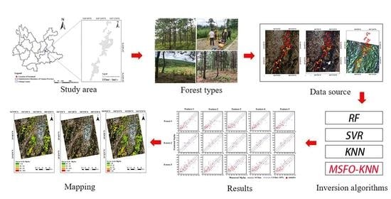
We conducted the field campaign in August 2019. In total, 78 samples were measured using the angle count method. The AGB values were calculated for 1 ha using transformation functions between stem volume ($V$) and AGB ($W$). During the field campaign, all trees greater than 5 cm dimeter at the breast height (DBH) at 1.3 m height were callipered, marked, and recorded tree species, number of the stems, and the height for each sampled plot. The locations of each angle count observing point were georeferenced by a differential global positioning system (GPS). The stem volumes for individual trees were calculated using a locally developed model [33]. The volume-AGB transformation functions of the individual tree species involved in this study were developed by Huang et al. as follows [34]:

$$W_1=0.8596V^{0.8564};W_2=0.5272V^{1.0793};W_3=0.1807V^{1.2771};W_4=0.6573V^{1.0502}$$

(1)

where $W_1$ indicates Yunnan Pines; $W_2$ indicates Huashan Pines; $W_3$ indicates Chinese fir; $W_4$ indicates other tree species.

The AGB information of the surveyed samples in this study were classified in three classes according to forest types.

Table 5. Statistics for the 78 plots.

Forest Type	Number	AGB (Mg/ha) Above-Ground Biomass	Mean (Mg/ha)	Standard (Mg/ha)
Forest-1	55	9.34~135.71	44.90	28.11
Forest-2	23	42.30~150.71	80.60	30.72
Forest-3	78	9.34~150.34	55.42	33.17

shows the details of AGB for the classified three forest types.

3. Methodology

The idea of proposed MSFO-KNN is motivated by combing the advantages of RF and KNN machine learning methods. RF is used for its excellent feature optimization capability and the fast speed of processing in the field of feature selection through measuring the variable importance in different ways. However, RF involves hierarchical structure problems and suffers the weakness of a complex and unstable implement coming from each decision tree during vegetation inversion using RS datasets. Inverse KNN is independent of the distribution of the feature and is simple and stable to implement the retrieval of the vegetation parameter, but it suffers the curse of dimensionality especially when high dimension RS features are involved. Thus, combination variable importance calculation function and the capability of KNN inversion may result in stabled and efficient vegetation parameter inversion, especially using high dimension RS variables. Nevertheless, the combination of RF and KNN still need further removal of uncertain variables and identification of the best combination of the selected important features during the forest parameter inversion procedure. Here, we embedded fast iterative procedure in KNN for best feature combination selection, and then the MSFO-KNN was proposed and presented. The procedure for forest AGB estimation using the MSFO-KNN algorithm was illustrated in Figure 2.

3.1. Random Forest (RF) for Original Remote Sensing Feature Optimization

Variable importance of RF is indicated by mean decrease in Gini (MDG) and mean decrease in accuracy (MDA). The MDG indicates the Gini impurity metric reduction by a variable in a certain class or retrieval level, while MDA measures the difference between out-of-bag errors obtained through random permutations of the values of the input RS variables and that resulting from the original data set. In this paper, the importance of the extracted RS features was implemented in R software with the importance function [35] and the relationship between the selected feature numbers and the estimated forest biomass accuracies.

3.2. Feature Combination Obtained with a Fast Iterative Procedure Embedded in KNN Algorithms

The performance efficiency of KNN is affected by the value of K, the curse of feature dimensionality, and the irrelevant RS features. In this paper, the values of K were set between 1~11 according to previous studies [26,27], and a fast iterative procedure was introduced to improve the efficiency of each KNN for AGB estimation performance at the base of feature importance calculated by RF. The part was shown in Figure 2 as the method procedure. In Figure 2, $m$ is the number of extracted SAR features, while $n=78$ is the number of plots in this study.

(1)

The trained datasets comprised of the field samples and RF selected RS variables are defined as $F=\left\{f_1,f_2,\cdots ,f_m\right\}$, where $m$ describes the number of selected original RS variables after the ordering using the RF variable importance function. Among them, $f_j={\left[x_{j1},x_{j2},\cdots ,x_{jn},\right]}^T(1\le j\le m)$, $x_{ji}$ is the pixel value of the $jth$ feature character at the $ith$ plot, where $n$ is the plot number and $T$ means the transform of the vector.

(2)

Initializing the original best optimized feature subset as $F_s=\left\{null\right\},s=0$, and the root means square error (RMSE) for the best estimation model as $RMS{E}_0=150t/ha$, it is initialized according to the maximum AGB value at the study area.

(3)

Generate $m-s$ KNN models and their retrieval RMSE values by feature combinations of $\left\{f_1,F_s\right\},\left\{f_2,F_s\right\},\cdots ,\left\{f_{\mathrm{i}-1},F_s\right\},\left\{f_{\mathrm{i}+1},F_s\right\},\cdots ,and\left\{f_m,F_s\right\}$, where $\left(f_{\mathrm{i}}=F_s\cap F\right)$. The RMSE values are calculated with the leave one out cross validation (LOOCV) method.

(4)

The lowest value of RMSE calculated in step 3) is set as $RMS{E}_b$; if $RMS{E}_b\le RMS{E}_0$, then $RMS{E}_0=RMS{E}_b$ and the feature combination for the $RMS{E}_0$ is set for $F_s$.

(5)

Step 3 is repeated iterative times until $RMS{E}_b\ge RMS{E}_0$.

3.3. Forest Biomass Estimation and Validation Using Proposed MSFO-KNN

For forest biomass estimation, the RS image features were first ranked with RF variable importance calculation. Then, the relations between the feature numbers and biomass estimation RMSE values were plotted and applied for selection of the input feature numbers in the next step (introduced in Section 3.2), and the best performance was selected as the retrieval results.

In this study, we divided the forest into three types (Forest-1, Forest-2, and Forest-3). The RS features were organized into five groups (Feature-1, Feature-2, Feature-3, Feature-4, and Feature-5). Thus, the five best performances of the feature combination sets and related estimation models were conducted for forest biomass estimation of three forest types, respectively.

4. Results

4.1. Remote Sensing Features Optimization Analysis

4.1.1. Original Feature Ordering and Optimization by RF

Random forest (RF) for original RS feature optimization was applied for five groups of RS features. Figure 3 plots the relationships between the numbers of the extracted RS features and the biomass estimation RMSE values for the five feature groups and the three forest types. The relationships discussed here were used to improve the time-consuming problem of putting all RS features into the inversion models. For a given feature resource, although the trends followed a comparable structure, variation was obvious among different forest types. These differences might be explained by several factors, including the difference in forest structures, tree species, and features describing different scattering mechanisms of forest. For the three forest types, RMSE values of Forest-1 remained the lowest among them; next was Forest-3, and the worst was Forest-2. For Forest-1, the Yunnan pines were the only tree species and its forest structure was simple. Forest-2 had more complex tree species and forest structures compared to Forest-1 and Forest-3. As such, the trends of Forest-2 fluctuated more variably, especially when the number of the features was smaller. Meanwhile, the capability of characterization of each RS feature regarding the change of forest biomass might lead to the fluctuation of trends. Since the average biomass was low in the study area, features extracted from optical images showed better performance for forest AGB, which might be due to the dominant biomass existing at the forest canopy. All of the trends remained stable at number of 45 for each feature group, according to the trend observations in Figure 3; thus, the first 10, 20, 30 and 40 features in the importance lists were selected as input features for the next step of optimal feature selection and combination.

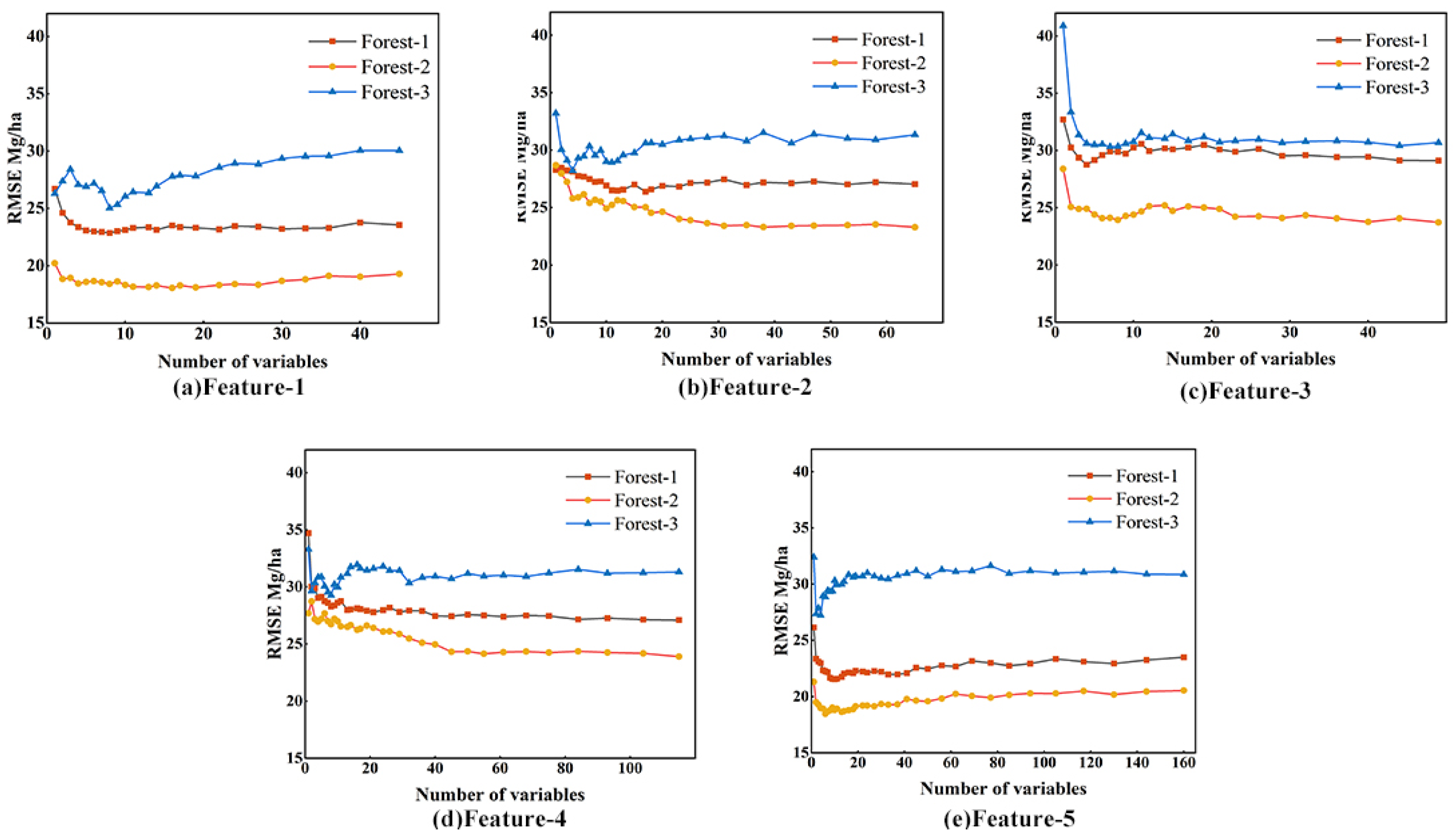
4.1.2. Second Step Feature Optimization by the Fast Iterative Procedure

The best combinations of the selected features coming from different resources according to their importance calculated in RF algorithms were generated by the fast iterative procedure for five feature groups including Feature-1, Feature-2, Feature-3, Feature-4, and Feature-5 (

Table 6. The optimized feature combinations and input parameters for forest AGB estimation.

Forest Types	Feature Groups	Numbers of Chosen Feature	Numbers of Feature	Selected Features
Forest-1	Feature-1	10	40	Green, Meg, Disr, Varb, Conr
	Feature-2	10	20	Blue, Green, Swir2, Swir1, Red, EVI, MidIR, Corg, Ens1, Meg
	Feature-3	8	40	L3, T22, T33, T23real, VVdB, H, $\lambda$, Mespan
	Feature-4	7	20	EVI, MidIR, Red, MSI, Meg, Mes2, Cons1
	Feature-5	5	30	BlueGF1, MidIRLad, Meg_GF1, NDVILad, RVILad
Forest-2	Feature-1	5	40	RVI, Varg, Varb, Disr, Conb
	Feature-2	4	20	Homos2, Corr, Ens2, Vars1
	Feature-3	5	20	T23imag, $\beta$, L3, Asmspan, Dissspan, Yam_OdddB
	Feature-4	4	20	Mer, Homos2, Vars2, Yam_DbldB
	Feature-5	4	10	GreenGF1, Asms2_GF1, Corr_GF1, H1
Forest-3	Feature-1	4	40	Blue, red, Conr, Cong
	Feature-2	5	20	RVI, MidIR, SR, NDVI, Cons1
	Feature-3	5	40	Yam_VoldB, A, T13imag, T33dB, Conspan
	Feature-4	5	40	VARI, Swir1, Ens1, Vars2, H2
	Feature-5	3	10	GreenGF1, RedGF1, RedLad

Subscripts were added for each texture feature to distinguish which image they are extracted from, for example, r, g, b, n, s1, s2 in subscripts means texture features extracted from red, green, blue, near-infrared, mid-infrared bands and far-infrared bands from the Landsat8 image, while when they were extracted from GF-1, the subscripts were added the contents of GF-1 into r, g, b, and n, respectively.

).

Among the five feature groups and three forest types, the features chosen in the optimal feature subsets were no more than 10, and the features were selected mostly from the first 20 important features in the importance lists. The selected features for different RS sources and forest types were changeable; however, for Feature-4 and Feature-5, more features from optical images were chosen than that extracted from SAR images. This revealed that optical features performed better for forest biomass estimation than C-band SAR features in our study area. Moreover, more texture features were selected from GF-1 for Forest-1, while more spectral features were selected from Landsat8. However, for Forest-2, the selected features from both GF-1 and Landsat8 were texture features. For Forest-3, the selected features from Landsat8 included vegetation indices, spectral features, and texture features as well. Conversely, for GF-1, only several spectral features and texture features were chosen. The differences were also shown in the selected features from the combination of optical and SAR features. Among the selected optical features from the feature combinations, spectral features performed better in Forest-3, while texture features performed better in Forest-2.

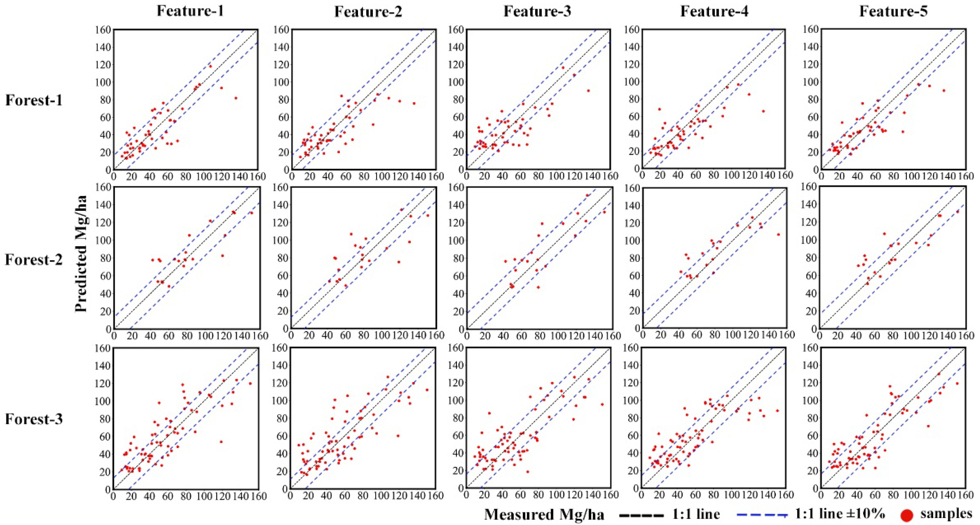
4.1.3. Forest AGB Retrievals Using Different Nonparametric Algorithms

After selecting the best combination of the features, in this section we retrieved forest biomass using the proposed MSFO-KNN algorithm, which was then compared to the performance of traditional machine learning algorithms, including KNN, SVR, and RF. KNN, SVR, and RF algorithms used here were trained by randomly selecting n-1 samples and validated using the remaining one sample for n times.

For the MSFO-KNN algorithm, the optimal K values, R² and RMSE values for each feature group and each forest type were determined, considering the minimum RMSE between the estimated and ground measured biomass. The detailed information is listed in

Table 7. The detailed information of the performance of the MSFO-KNN algorithm.

Forest Type	Feature Group	R2	RMSE
Forest-1	Feature-1	0.68	16.27
	Feature-2	0.63	18.05
	Feature-3	0.57	18.87
	Feature-4	0.63	18.25
	Feature-5	0.70	16.18
Forest-2	Feature-1	0.71	17.01
	Feature-2	0.56	20.96
	Feature-3	0.70	18.60
	Feature-4	0.70	18.27
	Feature-5	0.72	17.66
Forest-3	Feature-1	0.68	19.75
	Feature-2	0.60	21.79
	Feature-3	0.60	21.87
	Feature-4	0.62	21.34
	Feature-5	0.71	18.67

. For Forest-1, the chosen features and the proposed algorithm were most sensitive to biomass change and the best retrieval accuracy (R² values ranged from 0.57 to 0.70, and RMSE varied from 16.18 Mg/ha to 18.87 Mg/ha) was reported. For Forest-2, estimates correlated strongly with the observed biomass (R²: 0.56~0.72; RMSE: 17.66~20.96 Mg/ha). Correlations were slightly weaker for Forest-3 than the other two groups; the lower correlations might result from the greater dispersion of forest structure distributions. For feature groups, taking advantage of inputs of multiple source parameters, using Feature-5 improved the capability of forest biomass estimate. Correlations for three forest types were highest compared with other groups (R² = 0.70 for Forest-1, R² = 0.72 for Forest-2, and R² = 0.71 for Forest-3). This group had the lowest RMSE values as well (RMSE = 16.18 Mg/ha for Forest-1, RMSE =17.66 Mg/ha for Forest-2, and RMSE = 18.67 Mg/ha for Forest-3).

Figure 4 graphed the biomass retrieved using MSFO-KNN specified for forest types and feature groups against ground measured samples. Agreement line (1:1 line) was shown in each scatterplot for the equivalency of observed and predicted forest AGB values. The estimated dynamic ranges for Forest-1 were around 90 Mg/ha, except the results retrieved by Feature-3 with the decreased dynamic range of around 60 Mg/ha, and the results retrieved by Feature-5 with the increased dynamic range of around 120 Mg/ha. The dynamic range decrease might result from the low saturation of the C-band and its weak sensitivity to forest biomass changes, while the reason for the increased dynamic range could be the better sensitivity of optical information to the changes of forest biomass. The better performance of optical than SAR features might result from the quite open forest in the study area, where the ground component dominates the total backscatter from the forest stands. Note that the dynamic range of the results acquired by Feature-3 for Forest-2 was the widest among the five feature groups, with the value around 120 Mg/ha. It revealed the better performance of SAR source features to estimate mixed forest type. Conversely, the features extracted from Feature-1 performed better and were more stable in each forest type (R² = 0.68 for Forest-1, R² = 0.71 for Forest-2, and R² = 0.68 for Forest-3; RMSE = 16.27 Mg/ha for Forest-1, RMSE =17.01 Mg/ha for Forest-2, and RMSE = 19.75 Mg/ha for Forest-3).

To better understand the performance of the proposed MSFO-KNN algorithm, we retrieved the forest biomass using the RF, SVR, and KNN algorithms. The results estimated by them are summarized in

Table 8. The detailed information of the performance of the RF, SVR, and KNN algorithms.

Method	Forest Type	Feature Group	R2	RMSE
RF	Forest-1	Feature-1	0.62	17.42
		Feature-2	0.39	22.01
		Feature-3	0.15	26.03
		Feature-4	0.33	23.51
		Feature-5	0.61	17.91
	Forest-2	Feature-1	0.37	26.91
		Feature-2	0.30	26.29
		Feature-3	0.24	31.65
		Feature-4	0.13	32.55
		Feature-5	0.27	28.55
	Forest-3	Feature-1	0.57	22.09
		Feature-2	0.33	28.38
		Feature-3	0.31	28.21
		Feature-4	0.36	27.37
		Feature-5	0.61	20.78
SVR	Forest-1	Feature-1	0.59	21.47
		Feature-2	0.39	26.11
		Feature-3	0.30	27.93
		Feature-4	0.41	25.83
		Feature-5	0.61	20.83
	Forest-2	Feature-1	0.59	18.04
		Feature-2	0.50	20.01
		Feature-3	0.36	22.41
		Feature-4	0.42	21.52
		Feature-5	0.64	16.91
	Forest-3	Feature-1	0.27	26.41
		Feature-2	0.25	26.79
		Feature-3	0.20	31.89
		Feature-4	0.32	25.49
		Feature-5	0.49	22.36
KNN	Forest-1	Feature-1	0.22	30.78
		Feature-2	0.10	36.60
		Feature-3	0.27	28.03
		Feature-4	0.08	33.32
		Feature-5	0.31	26.96
	Forest-2	Feature-1	0.35	25.59
		Feature-2	0.33	25.77
		Feature-3	0.13	25.79
		Feature-4	0.18	26.42
		Feature-5	0.48	22.15
	Forest-3	Feature-1	0.45	25.70
		Feature-2	0.29	29.09
		Feature-3	0.25	30.67
		Feature-4	0.34	28.50
		Feature-5	0.64	21.02

and Figure 5. For the setting of model parameters of the trained RF, SVR, and KNN, detailed information was given in Tables S1 and S2 and Figure S1 in the Supplementary Materials, respectively.

The RF was designed with ntree values less than 2000 and mtry values set as one third of the input features. Table 8 and Figure 5a show the comparison of the retrieved and ground identified forest AGB for each feature group and forest type. The RF did not perform as well as the MSFO-KNN. The RMSE values were higher and the R² values acquired at each feature group and each forest type were lower, compared with the values acquired by the MSFO-KNN algorithms. Certain input features without removal appeared in multiple trees in RF, which might cause the weak estimate. Nevertheless, the estimated forest results from RF using Feature-1 matched well with the measured values, with an R² close to those obtained by MSFO-KNN algorithms.

The SVR algorithms with the best model parameters were applied for predicting AGB. The model parameters differed with the change of the feature group. According to Table 8 and Figure 5a,b. Similar AGB retrieval results were observed for SVR with RF; the retrieved values using Feature-1 and Feature-5 matched better with ground measurements (for Feature-1: R² = 0.62 for Forest-1, R² = 0.37 for Forest-2, and R² = 0.57 for Forest-3; RMSE = 17.42 Mg/ha for Forest-1, RMSE = 26.91 Mg/ha for Forest-2, and RMSE = 22.09 Mg/ha for Forest-3; for Feature-5: R² = 0.61 for Forest-1, R² = 0.27 for Forest-2, and R² = 0.61 for Forest-3; RMSE = 17.91 Mg/ha for Forest-1, RMSE = 28.55 Mg/ha for Forest-2, and RMSE = 20.78 Mg/ha for Forest-3), while both of these two group features showed the worst performance in Forest-2. Figure 5b depicts scatterplots of predicted biomass by SVR versus ground measured values. The patterns of the scatterplots showed similar scattering modes with Figure 5a, and most of them showed underestimation at the higher AGB levels.

The results from the application of Mahalanobis distance with the KNN algorithm are shown in Table 8 and Figure 5c. The number of neighbors (K) were chosen according to the relations between retrieved biomass RMSE values and K values. The scatterplots in Figure 5c revealed an obvious underestimation of the estimates at all three forest types, especially for Forest-1, the underestimation phenomenon showed in each feature group working as inputs. However, a few of them showed better performance, like in Forest-3 using features of Feature-5 (R² = 0.64; RMSE = 21.02 Mg/ha).

According to the comparison of the performances of the proposed MSFO-KNN and RF, SVR, and KNN applied in three forest types with five feature groups, it was obvious that the MSFO-KNN outperformed the RF, SVR, and KNN algorithms, particularly for three forest types using features coming from Feature-2, Feature-3, and Feature-4. Different nonparametric approaches required different optimal numbers of training data and input features to derive their estimators; their influence was obvious to RF, SVR, and KNN algorithms, while it had weaker effects on the MSFO-KNN algorithm since it performed similarly for each feature group with its estimates.

Figure 6 displayed the spatial distribution maps acquired by the MSFO-KNN algorithm using RS features coming from Feature-5 in the entire study area with three forest types. AGB values higher than 200 Mg/ha and lower than 0 Mg/ha were assumed overestimates and underestimates of the real biomass range in the test site and were excluded. For Forest-1, the retrieved AGB seemed more homogenous (around 70% of them ranged from 30~60 Mg/ha), with only very few beyond 90 Mg/ha (around 10%) and lower than 30 Mg/ha (around 20%). The AGB spatial application of Forest-2 depicted some variation, with 40% of them ranging between 30~60 Mg/ha, and 40% ranging between 60~90 Mg/ha. The AGB spatial distribution of Forest-3 were similar to Forest-1, with around 70% of them ranging between 30~60 Mg/ha.

5. Discussion

5.1. Capabilities and Limitations of the Features Extracted from Optical and SAR Images

Two optical feature groups, like Feature-1 and Feature-2, were applied to retrieve the forest biomass. The features coming from Feature-1 and Feature-2 showed different performances in the estimation. For Feature-1, more texture features were chosen for the last feature combination regarding the highest forest biomass estimation accuracy. Meanwhile, several texture features coming from Feature-2 measured the biomass of Forest-2 better than the original band features. These findings agreed with Ou et al., who investigated Pinus densata forest AGB estimation with optical images [15]. The better performance of Feature-1 compared to Feature-2 might also result from the higher spatial resolution of GF-1 than that of Landsat8. The chosen optimal SAR features in this study included backscatter coefficients, polarimetric decomposition features, and texture features as well. Among them, more backscatter coefficients were chosen as optimal features for Forest-1 AGB estimation, while more texture and polarimetric features were chosen for Forest-2 AGB estimation. The texture and polarimetric features extracted from the L-band SAR image also showed good performance in AGB estimation in Larix gmelinii and Betula platyphylla mixed forest [27], while the C-band GF-3 polarimetric features performed well in forest canopy AGB retrieval, with the highest R² = 0.658 and the lowest RMSE value of 4. 943 t/hm⁻² [36].

We carried out further quantitative analysis by comparing the estimate results through the features from five different groups (Table 8 and Figure 5). The highest R² and RMSE values using Feature-1 and Feature-2 were R² = 0.71 with RMSE = 17.01 Mg/ha, and R² = 0.63 with RMSE = 18.05 Mg/ha, respectively. The values using Feature-3 were R² = 0.70 with RMSE =18.60 Mg/ha, while the combination of both optical and SAR features (Feature-5) obtained the highest R² (0.72) and lowest RMSE (16.18 Mg/ha) values. Moreover, the estimation accuracies using optical and SAR feature combination for each forest group were also higher than the corresponding accuracy using Feature-1, Feature-2, and Feature-3. For optical features, the better group, Feature-1, had better performance in each forest type than the corresponding accuracies acquired by using features from Feature-3, the SAR features. The better performance of optical features in forest biomass retrieval might result from the integration of optical textures and spectral response in biomass estimation [13,16], whereas the worse performance of SAR features was due to the C-band’s inability to capture the change forest biomass [13,26].

5.2. Differences between Forest Types on AGB Estimation

Forest structure AGB trends differed between forest types, and the trends led to the variation of forest AGB estimation accuracy using RS features [37]. The obvious differences between Forest-1, Forest-2, and Forest-3 concerned tree species and biomass level variety in our study area. As a result, the selected optimal feature subsets differed for Forest-1, Forest-2, and Forest-3 (Table 6). The effects of the differences between Forest-1, Forest-2, and Forest-3 on the estimate results were quantitatively explored; the estimates considering no effect of forest type were conducted as Forest-3, and the results were then compared with the individual results of Forest-1 and Forest-2, which considered the effects of forest type. Figure 6 compared the performance of RF, SVR, and KNN using five RS feature sets. Figure 6 showed that the average overall accuracy of Forest-1 was highest in most cases compared with Forest-2 and Forest-3, with the lowest average RMSE value of 17.52 Mg/ha acquired with the MSFO-KNN algorithm. Moreover, it also had the lowest RMSE values compared with Forest-2 and Forest-3, even using RF, SVR, and KNN algorithms. Since Forest-1 was composed of almost entirely a single tree species, and was therefore more homogeneous than Forest-3, and especially Forest-2, then the forest structure of Forest-1 is simpler than that of Forest-2 and Forest-3 as a result. Higher AGB estimation accuracy was acquired in Forest-1 than in Forest-2 and Forest-3. Previous studies also demonstrated the importance of taking the forest structure into account for a given species and a given level of forest biomass [2,6,14].

5.3. Performance of the Proposed MSFO-KNN Algorithm

The performance of MSFO-KNN was compared with the results of RF, SVR, and KNN (Figure 7 and Figure 8). The average R² values and RMSE values calculated by the average resulted obtained by RF, SVR, and KNN were shown in Figure 7, they revealed their weak performance in complex forest types like Forest-3. Compared with their performance, as the RMSE values shown in Figure 8, MSFO-KNN showed better performance in forest AGB estimation. The comparison in Figure 8 revealed its weak dependence on RS images and forest structures. Among the five feature groups, the MSFO-KNN algorithm performed best in improving the estimate accuracy by using the features extracted from GF-3; the next was the Landsat8 image, and then the feature combination of them. For the three forest types, Forest-2 often showed the worst estimation accuracy compared with Forest-1 and Forest-3, while its accuracy was greatly improved when using MSFO-KNN. Most of the R² values were higher than Forest-3, and RMSE values were lower than Forest-3. Previous studies demonstrated that a comparison of retrieval algorithms was very valuable. they also proposed that to know the uncertainties resulting from satellite imagery differences was important as well [6,38]. Their results confirmed the different performance of each algorithm and also their dependence with the forest AGB levels. The results also highlighted the better performance of SVR for the lower forest AGB level (less than 260 Mg/ha). These findings were comparable to the results of this study, proving that the estimation accuracy depends on the retrieval algorithms.

6. Conclusions

In this study, a GF1 image, a Landsat8 image, and a GF3 image covering the study area were collected and then used to estimate forest biomass. The RS features extracted from optical and SAR data were divided into five groups and applied for three different forest type group (Forest-1, Forest-2, and Forest-3) to obtain biomass estimates. We proposed the MSFO-KNN algorithm for forest biomass estimation, and its performance was compared with RF, SVR, and KNN; during the procedure, the forest type and feature combination effects were considered. Some conclusions were obtained: (1) Textures played a more important role than spectral bands in forest AGB modeling. (2) Features extracted from GF1 imagery provided more accurate estimates of AGB than features coming from other RS data, especially when the traditional nonparametric models were applied. The combination of GF1 features with other imagery features had limited effects on improving AGB estimation; however, it showed obvious dependence on retrieval algorithms. (3) It was shown that all of the AGB retrieval models performed best in Forest-1, but worst in Forest-2 or Forest-3. Thus, it was important to consider the effects of forest type in forest AGB estimation, especially using the traditional nonparametric algorithms. (4) The superiority of the proposed MSFO-KNN algorithm was validated by comparing it with RF, SVR, and KNN in forest AGB estimation. The overall AGB estimation accuracies achieved were the highest and the RMSE values were lowest for each forest type and using each RS feature group. The results also revealed its non-dependence on the data source and forest type. In the future, further validation will be conducted at more forest sites, and more consideration should focus on the influence of AGB level variety.

References

1. Stocker, T.; Qin, D.; Plattner, G.-K.; Tignor, M.; Allen, S.K.; Boschung, J.; Nauels, A.; Xia, Y.; Bex, V.; Midgley, P.M.; et al. Climate Change 2013—The Physical Science Basis: Working Group I Contribution to the Fifth Assessment Report of the Intergovernmental Panel on Climate Change; IPCC, Ed.; Cambridge University Press: Cambridge, UK, 2014; ISBN 978-1-107-41532-4. [Google Scholar]
2. Le Toan, T.; Quegan, S.; Davidson, M.W.J.; Balzter, H.; Paillou, P.; Papathanassiou, K.; Plummer, S.; Rocca, F.; Saatchi, S.; Shugart, H.; et al. The BIOMASS mission: Mapping global forest biomass to better understand the terrestrial carbon cycle. Remote Sens. Environ. 2011, 115, 2850–2860. [Google Scholar] [CrossRef] [Green Version]
3. Soja, M.J.; Quegan, S.; d’Alessandro, M.M.; Banda, F.; Scipal, K.; Tebaldini, S.; Ulander, L.M.H. Mapping above-ground biomass in tropical forests with ground-cancelled P-band SAR and limited reference data. Remote Sens. Environ. 2021, 253, 112153. [Google Scholar] [CrossRef]
4. Hayashi, M.; Motohka, T.; Sawada, Y. Aboveground Biomass Mapping Using ALOS-2/PALSAR-2 Time-Series Images for Borneo’s Forest. IEEE J. Sel. Top. Appl. Earth Obs. Remote Sens. 2019, 12, 5167–5177. [Google Scholar] [CrossRef]
5. Lu, D.; Chen, Q.; Wang, G.; Moran, E.; Batistella, M.; Zhang, M.; Vaglio Laurin, G.; Saah, D. Aboveground Forest Biomass Estimation with Landsat and LiDAR Data and Uncertainty Analysis of the Estimates. Int. J. For. Res. 2012, 2012, 436537. [Google Scholar] [CrossRef]
6. Gao, Y.; Lu, D.; Li, G.; Wang, G.; Chen, Q.; Liu, L.; Li, D. Comparative Analysis of Modeling Algorithms for Forest Aboveground Biomass Estimation in a Subtropical Region. Remote Sens. 2018, 10, 627. [Google Scholar] [CrossRef] [Green Version]
7. Rodríguez-Veiga, P.; Quegan, S.; Carreiras, J.; Persson, H.J.; Fransson, J.E.S.; Hoscilo, A.; Ziółkowski, D.; Stereńczak, K.; Lohberger, S.; Stängel, M.; et al. Forest biomass retrieval approaches from earth observation in different biomes. Int. J. Appl. Earth Obs. Geoinf. 2019, 77, 53–68. [Google Scholar] [CrossRef]
8. Chowdhury, T.; Thiel, C.; Schmullius, C.; Stelmaszczuk-Górska, M. Polarimetric Parameters for Growing Stock Volume Estimation Using ALOS PALSAR L-Band Data over Siberian Forests. Remote Sens. 2013, 5, 5725–5756. [Google Scholar] [CrossRef] [Green Version]
9. Foody, G.M.; Boyd, D.S.; Cutler, M.E.J. Predictive relations of tropical forest biomass from Landsat TM data and their transferability between regions. Remote Sens. Environ. 2003, 85, 463–474. [Google Scholar] [CrossRef]
10. Mitchard, E.T.A.; Saatchi, S.S.; Lewis, S.L.; Feldpausch, T.R.; Woodhouse, I.H.; Sonké, B.; Rowland, C.; Meir, P. Measuring biomass changes due to woody encroachment and deforestation/degradation in a forest–savanna boundary region of central Africa using multi-temporal L-band radar backscatter. Remote Sens. Environ. 2011, 115, 2861–2873. [Google Scholar] [CrossRef] [Green Version]
11. Godinho Cassol, H.L.; De Oliveira E Cruz De Aragão, L.E.; Moraes, E.C.; De Brito Carreiras, J.M.; Shimabukuro, Y.E. Quad-pol advanced land observing satellite/phased array L-band synthetic aperture radar-2 (ALOS/PALSAR-2) data for modelling secondary forest above-ground biomass in the central Brazilian Amazon. Int. J. Remote Sens. 2021, 42, 4985–5009. [Google Scholar] [CrossRef]
12. Montesano, P.M.; Cook, B.D.; Sun, G.; Simard, M.; Nelson, R.F.; Ranson, K.J.; Zhang, Z.; Luthcke, S. Achieving accuracy requirements for forest biomass mapping: A spaceborne data fusion method for estimating forest biomass and LiDAR sampling error. Remote Sens. Environ. 2013, 130, 153–170. [Google Scholar] [CrossRef]
13. Li, Y.; Li, M.; Li, C.; Liu, Z. Forest aboveground biomass estimation using Landsat 8 and Sentinel-1A data with machine learning algorithms. Sci. Rep. 2020, 10, 9952. [Google Scholar] [CrossRef] [PubMed]
14. Lu, D. The potential and challenge of remote sensing-based biomass estimation. Int. J. Remote Sens. 2006, 27, 1297–1328. [Google Scholar] [CrossRef]
15. Ou, G.; Li, C.; Lv, Y.; Wei, A.; Xiong, H.; Xu, H.; Wang, G. Improving Aboveground Biomass Estimation of Pinus densata Forests in Yunnan Using Landsat 8 Imagery by Incorporating Age Dummy Variable and Method Comparison. Remote Sens. 2019, 11, 738. [Google Scholar] [CrossRef] [Green Version]
16. Lu, D.; Chen, Q.; Wang, G.; Liu, L.; Li, G.; Moran, E. A survey of remote sensing-based aboveground biomass estimation methods in forest ecosystems. Int. J. Digit. Earth 2016, 9, 63–105. [Google Scholar] [CrossRef]
17. Sandberg, G.; Ulander, L.M.H.; Fransson, J.E.S.; Holmgren, J.; Le Toan, T. L- and P-band backscatter intensity for biomass retrieval in hemiboreal forest. Remote Sens. Environ. 2011, 115, 2874–2886. [Google Scholar] [CrossRef]
18. Chen, L.; Wang, Y.; Ren, C.; Zhang, B.; Wang, Z. Assessment of multi-wavelength SAR and multispectral instrument data for forest aboveground biomass mapping using random forest kriging. For. Ecol. Manag. 2019, 447, 12–25. [Google Scholar] [CrossRef]
19. Ji, Y.; Xu, K.; Zeng, P.; Zhang, W. GA-SVR Algorithm for Improving Forest Above Ground Biomass Estimation Using SAR Data. IEEE J. Sel. Top. Appl. Earth Obs. Remote Sens. 2021, 14, 6585–6595. [Google Scholar] [CrossRef]
20. Feng, Y.; Lu, D.; Chen, Q.; Keller, M.; Moran, E.; dos-Santos, M.N.; Bolfe, E.L.; Batistella, M. Examining effective use of data sources and modeling algorithms for improving biomass estimation in a moist tropical forest of the Brazilian Amazon. Int. J. Digit. Earth 2017, 10, 996–1016. [Google Scholar] [CrossRef]
21. Yang, Z.; Shao, Y.; Li, K.; Liu, Q.; Liu, L.; Brisco, B. An improved scheme for rice phenology estimation based on time-series multispectral HJ-1A/B and polarimetric RADARSAT-2 data. Remote Sens. Environ. 2017, 195, 184–201. [Google Scholar] [CrossRef]
22. Fleming, A.L.; Wang, G.; McRoberts, R.E. Comparison of methods toward multi-scale forest carbon mapping and spatial uncertainty analysis: Combining national forest inventory plot data and landsat TM images. Eur. J. For. Res. 2015, 134, 125–137. [Google Scholar] [CrossRef]
23. Breidenbach, J.; Næsset, E.; Gobakken, T. Improving k-nearest neighbor predictions in forest inventories by combining high and low density airborne laser scanning data. Remote Sens. Environ. 2012, 117, 358–365. [Google Scholar] [CrossRef]
24. McRoberts, R.E.; Chen, Q.; Domke, G.M.; Næsset, E.; Gobakken, T.; Chirici, G.; Mura, M. Optimizing nearest neighbour configurations for airborne laser scanning-assisted estimation of forest volume and biomass. Forestry 2017, 90, 99–111. [Google Scholar] [CrossRef]
25. Tian, X.; Su, Z.; Chen, E.; Li, Z.; van der Tol, C.; Guo, J.; He, Q. Estimation of forest above-ground biomass using multi-parameter remote sensing data over a cold and arid area. Int. J. Appl. Earth Obs. Geoinf. 2012, 14, 160–168. [Google Scholar] [CrossRef]
26. Han, Z.; Jiang, H.; Wang, W.; Li, Z.; Chen, E.; Yan, M.; Tian, X. Forest Above-Ground Biomass Estimation Using KNN-FIFS Method Based on Multi-Source Remote Sensing Data. Sci. Silvae Sin. 2018, 54, 70–79. [Google Scholar] [CrossRef]
27. Li, Y.; Zhang, W.; Cui, Y. Retrieval of Forest Aboveground biomass from optical and SAR data supported by parameter optimization. J. Beijing For. Univ. 2020, 42, 11–19. [Google Scholar]
28. Bu, F. Estimation of Forest Aboveground Biomass Based on Multi-Source Remote Sensing Data; Nanjing University of Information Engineering: Nanjing, China, 2019. [Google Scholar]
29. Jensen, J.R.; Lulla, K. Introductory digital image processing: A remote sensing perspective. Geocarto Int. 1987, 2, 65. [Google Scholar] [CrossRef]
30. Freeman, A.; Durden, S.L. A three-component scattering model for polarimetric SAR data. IEEE Trans. Geosci. Remote Sens. 1998, 36, 963–973. [Google Scholar] [CrossRef] [Green Version]
31. Yamaguchi, Y.; Moriyama, T.; Ishido, M.; Yamada, H. Four-component scattering model for polarimetric SAR image decomposition. Tech. Rep. Ieice Sane 2005, 104, 1699–1706. [Google Scholar] [CrossRef]
32. Cloude, S.R.; Pottier, E. A review of target decomposition theorems in radar polarimetry. IEEE Transac. Geosci. Remote Sens. 1996, 34, 498–518. [Google Scholar] [CrossRef]
33. Meng, X. Forest Mensuration; China Forestry Publishing House: Beijing, China, 2006; Volume 241–245, ISBN 978-1-4020-5990-2. [Google Scholar]
34. Huang, C.; Zhang, J.; Yang, W.; Tang, X.; Zhao, A. Dynamics on forest carbon stock in Sichuan Province and Chongqing City. Acta Ecol. Sin. 2008, 28, 0966–0975. [Google Scholar]
35. Belgiu, M.; Drăguţ, L. Random forest in remote sensing: A review of applications and future directions. ISPRS J. Photogramm. Remote Sens. 2016, 114, 24–31. [Google Scholar] [CrossRef]
36. Wei, J.; Fan, Y.; Yu, Y. Estimation of canopy biomass by polarimetric decomposition of GF-3 full polarimetric SAR data Forestry Science. Sci. Silvae Sin. 2020, 56, 10. [Google Scholar] [CrossRef]
37. Woodhouse, I.H.; Mitchard, E.T.A.; Brolly, M.; Maniatis, D.; Ryan, C.M. Radar backscatter is not a “direct measure” of forest biomass. Nat. Clim. Chang. 2012, 2, 556–557. [Google Scholar] [CrossRef]
38. Englhart, S.; Keuck, V.; Siegert, F. Modeling Aboveground Biomass in Tropical Forests Using Multi-Frequency SAR Data—A Comparison of Methods. IEEE J. Sel. Top. Appl. Earth Obs. Remote Sens. 2012, 5, 298–306. [Google Scholar] [CrossRef]
Figure 1. Map of Yunnan province with the location of Xiaoshao timberland. The top sub-panel shows the location of Yiliang county and the coverage of Xiaoshao timberland with the background of a Digital Elevation Model (DEM) map. The bottom sub-panel shows the distribution of collected stand plots with acquired RS images as background in this study. (a) Landsat8 (RGB = R, G, B), (b) GF1 (RGB = R, G, B), (c) GF3 with Pauli RGB.
Remotesensing 14 01608 g001
Figure 2. The flowchart for forest biomass estimation using the proposed MSFO-KNN algorithm.
Remotesensing 14 01608 g002
Figure 3. The relationships between the feature numbers and AGB estimation RMSE values.
Remotesensing 14 01608 g003
Figure 4. Forest AGB retrieval using the proposed MSFO-KNN algorithm.
Remotesensing 14 01608 g004
Figure 5. Forest AGB retrieval using the RF, SVR and KNN algorithms.
Remotesensing 14 01608 g005
Figure 6. AGB maps showing the spatial distribution generated by the MSFO–KNN algorithm in three forest types using features coming from Feature-5 at the study area.
Remotesensing 14 01608 g006
Figure 7. Comparison between the estimation accuracies of RF, SVR, and KNN using averaged values of five RS feature groups for three forest types.
Remotesensing 14 01608 g007
Figure 8. Comparison between the AGB estimation accuracies based on RF, SVR, KNN algorithms (a) and MSFO-KNN (b) using five groups of RS features in three forest types. The RMSE values of each bar in (a) indicates the average RMSE value of the estimation results of RF, SVR and KNN. The color difference describes the percentage of RMSE values of the results acquired by RF, SVR and KNN in the total RMSE values acquired by three algorithms.
Remotesensing 14 01608 g008