

Detecting the Auroral Oval through CSES-01 Electric Field Measurements in the Ionosphere
 ,
,  , ,
, ,  , , , ,
  and
and 
Abstract
:1. Introduction
2. Materials and Methods
2.1. Data
2.2. Electric Field Properties in the Auroral Oval
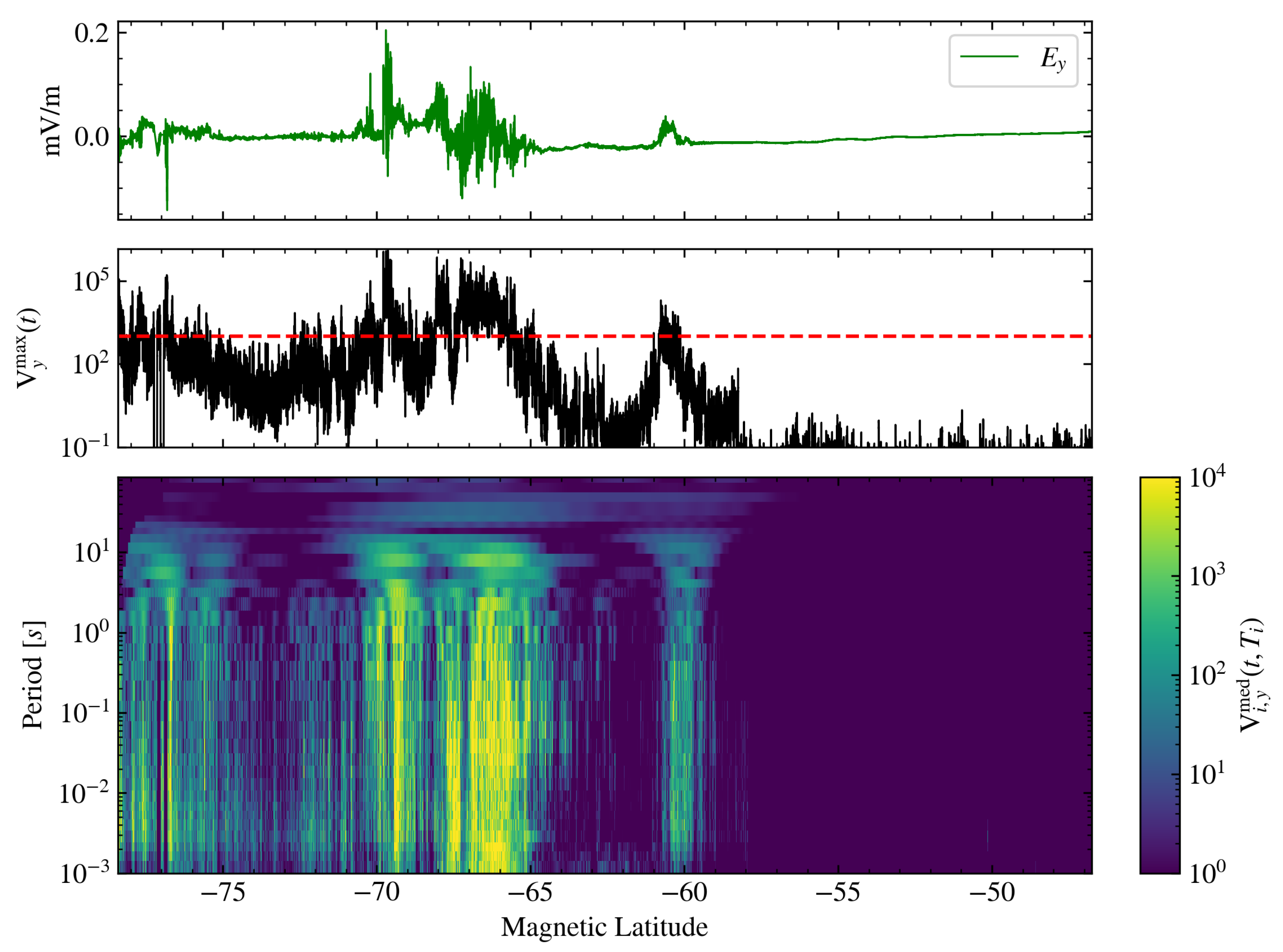
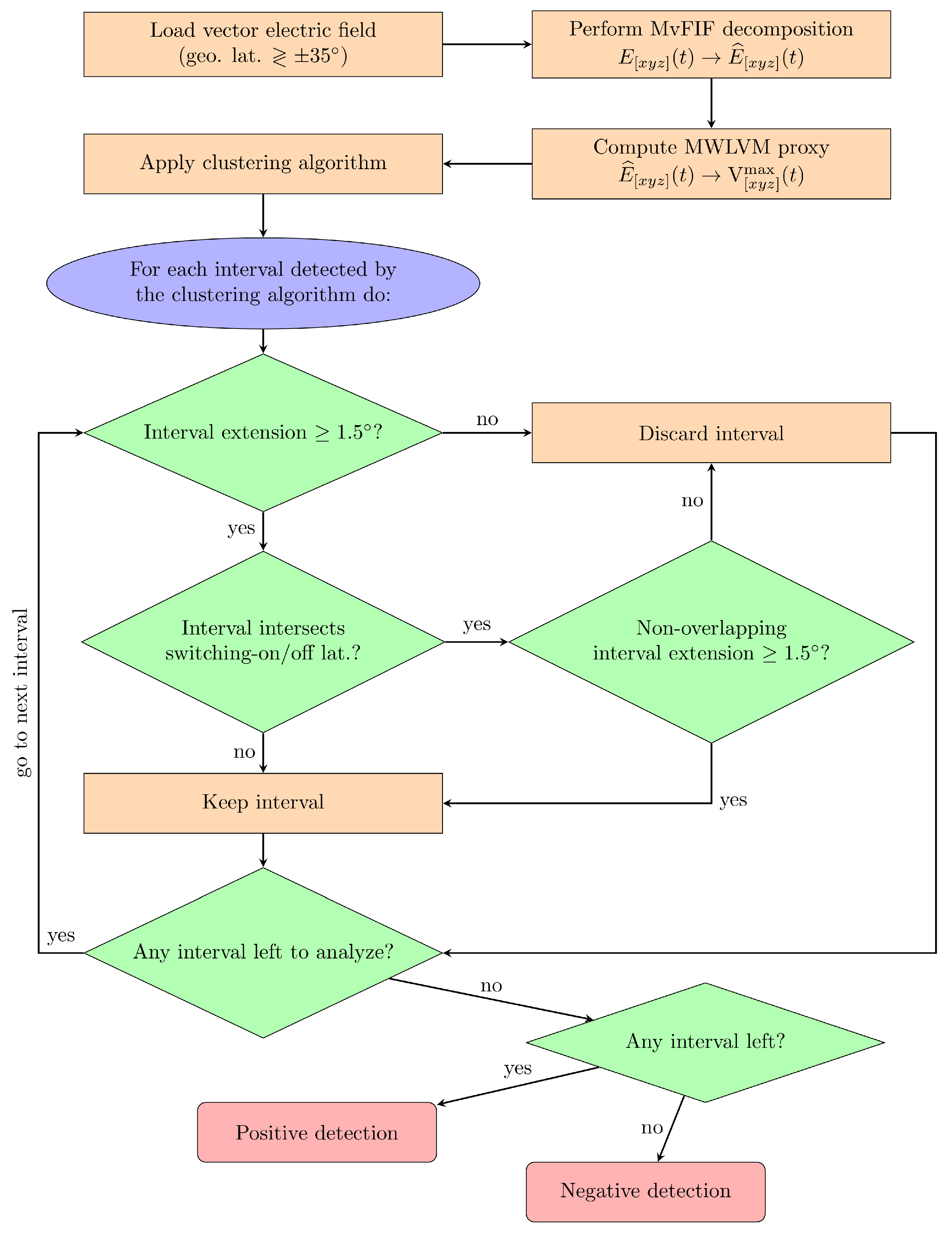
2.3. Auroral Oval Detection Based on a Local Variance Measure of the Electric Field
3. Results
3.1. Numerical Implementation
3.2. Validation of the Detection Algorithm
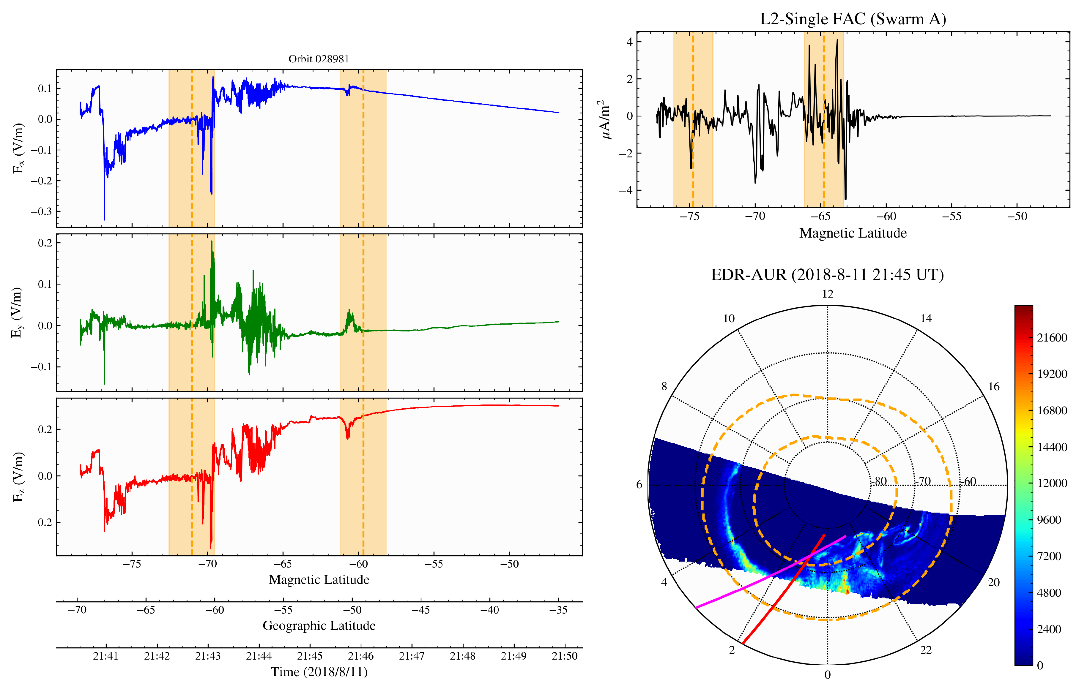
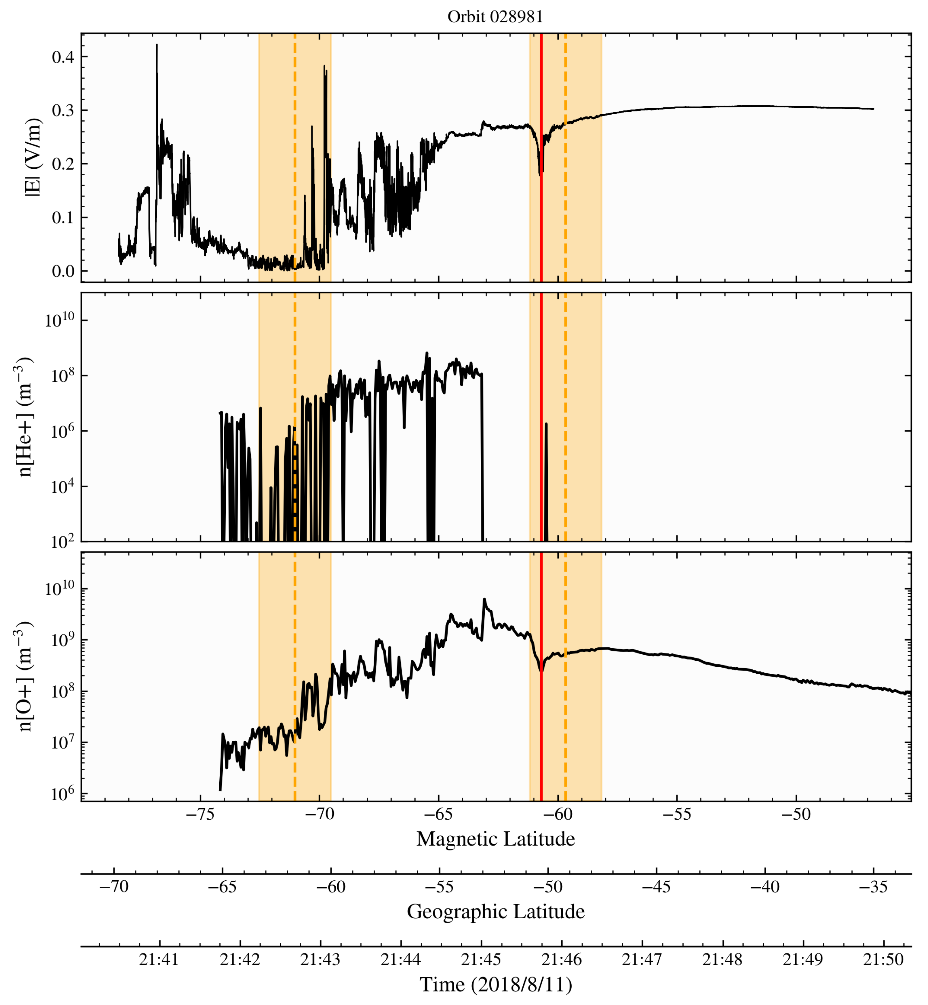
3.2.1. Southern Hemisphere
3.2.2. Northern Hemisphere
3.3. Polar Cap Detection
4. Discussion
Author Contributions
Funding
Data Availability Statement
Acknowledgments
Conflicts of Interest
References
- Borovsky, J.E.; Valdivia, J.A. The Earth’s Magnetosphere: A Systems Science Overview and Assessment. Surv. Geophys. 2018, 39, 817–859. [Google Scholar] [CrossRef] [PubMed] [Green Version]
- D’Angelo, G.; Piersanti, M.; Alfonsi, L.; Spogli, L.; Clausen, L.B.N.; Coco, I.; Li, G.; Baiqi, N. The response of high latitude ionosphere to the 2015 St. Patrick’s day storm from in situ and ground based observations. Adv. Space Res. 2018, 62, 638–650. [Google Scholar] [CrossRef]
- D’Angelo, G.; Piersanti, M.; Alfonsi, L.; Spogli, L.; Coco, I.; Li, G.; Baiqi, N. The response of high latitude ionosphere to the 2015 June 22 storm. Ann. Geophys. 2019, 62. [Google Scholar] [CrossRef] [Green Version]
- D’Angelo, G.; Piersanti, M.; Pignalberi, A.; Coco, I.; De Michelis, P.; Tozzi, R.; Pezzopane, M.; Alfonsi, L.; Cilliers, P.; Ubertini, P. Investigation of the Physical Processes Involved in GNSS Amplitude Scintillations at High Latitude: A Case Study. Remote Sens. 2021, 13, 2493. [Google Scholar] [CrossRef]
- Eastwood, J.P.; Nakamura, R.; Turc, L.; Mejnertsen, L.; Hesse, M. The Scientific Foundations of Forecasting Magnetospheric Space Weather. Space Sci. Rev. 2017, 212, 1221–1252. [Google Scholar] [CrossRef] [Green Version]
- Ganushkina, N.Y.; Liemohn, M.W.; Dubyagin, S. Current Systems in the Earth’s Magnetosphere. Rev. Geophys. 2018, 56, 309–332. [Google Scholar] [CrossRef]
- Gillies, D.M.; Knudsen, D.; Spanswick, E.; Donovan, E.; Burchill, J.; Patrick, M. Swarm observations of field-aligned currents associated with pulsating auroral patches. J. Geophys. Res. 2015, 120, 9484–9499. [Google Scholar] [CrossRef] [Green Version]
- Zou, Y.; Dowell, C.; Ferdousi, B.; Lyons, L.R.; Liu, J. Auroral Drivers of Large dB/dt During Geomagnetic Storms. Space Weather 2022, 20, e2022SW003121. [Google Scholar] [CrossRef]
- Paxton, L.J.; Meng, C.I.; Fountain, G.H.; Ogorzalek, B.S.; Darlington, E.H.; Gary, S.A.; Goldsten, J.O.; Kusnierkiewicz, D.Y.; Lee, S.C.; Linstrom, L.A.; et al. SSUSI: Horizon-to-horizon and limb-viewing spectrographic imager for remote sensing of environmental parameters. In Proceedings of the Ultraviolet Technology IV, San Diego, CA, USA, 20–21 July 1992; Society of Photo-Optical Instrumentation Engineers (SPIE) Conference Series. Huffman, R.E., Ed.; SPIE: Washington, DC, USA, 1993; Volume 1764, pp. 161–176. [Google Scholar] [CrossRef]
- Newell, P.T.; Feldstein, Y.I.; Galperin, Y.I.; Meng, C.I. Morphology of nightside precipitation. J. Geophys. Res. 1996, 101, 10737–10748. [Google Scholar] [CrossRef]
- Lunyushkin, S.; Penskikh, Y. Diagnostics of auroral oval boundaries on the basis of the magnetogram inversion technique. Sol.-Terr. Phys. 2019, 5, 88–100. [Google Scholar] [CrossRef]
- Edemskiy, I.K.; Yasyukevich, Y.V. Auroral Oval Boundary Dynamics on the Nature of Geomagnetic Storm. Remote Sens. 2022, 14, 5486. [Google Scholar] [CrossRef]
- Vorobev, A.; Pilipenko, V.; Krasnoperov, R.I.; Vorobeva, G.; Lorentzen, D.A. Short-term forecast of the auroral oval position on the basis of the “virtual globe” technology. Russ. J. Earth. Sci. 2020, 20, ES5007. [Google Scholar] [CrossRef]
- Cicone, A.; Pellegrino, E. Multivariate Fast Iterative Filtering for the Decomposition of Nonstationary Signals. IEEE Trans. Signal Process. 2022, 70, 1521–1531. [Google Scholar] [CrossRef]
- Huang, J.; Lei, J.; Li, S.; Zeren, Z.; Li, C.; Zhu, X.; Yu, W. The Electric Field Detector (EFD) onboard the ZH-1 satellite and first observational results. Earth Planet. Phys. 2018, 2, 469–478. [Google Scholar] [CrossRef]
- Shen, X.; Zhang, X.; Yuan, S.; Wang, L.; Cao, J.; Huang, J.; Zhu, X.; Piergiorgio, P.; Dai, J. The state-of-the-art of the China Seismo-Electromagnetic Satellite mission. Sci. China E: Technol. Sci. 2018, 61, 634–642. [Google Scholar] [CrossRef]
- Diego, P.; Huang, J.; Piersanti, M.; Badoni, D.; Zeren, Z.; Yan, R.; Rebustini, G.; Ammendola, R.; Candidi, M.; Guan, Y.B.; et al. The Electric Field Detector on Board the China Seismo Electromagnetic Satellite—In-Orbit Results and Validation. Instruments 2021, 5, 1. [Google Scholar] [CrossRef]
- Feldstein, Y.I. Auroral morphology, II. Auroral and geomagnetic disturbances. Tellus 1964, 16, 252–257. [Google Scholar] [CrossRef]
- Vorobjev, V.G.; Yagodkina, O.I. Seasonal and UT variations of the position of the auroral precipitation and polar cap boundaries. Geomagn. Aeron. 2010, 50, 597–605. [Google Scholar] [CrossRef]
- Wagner, D.; Neuhäuser, R. Variation of the auroral oval size and offset for different magnetic activity levels described by the Kp-index. Astron. Nachrichten 2019, 340, 483–493. [Google Scholar] [CrossRef]
- Consolini, G.; Quattrociocchi, V.; D’Angelo, G.; Alberti, T.; Piersanti, M.; Marcucci, M.F.; De Michelis, P. Electric Field Multifractal Features in the High-Latitude Ionosphere: CSES-01 Observations. Atmosphere 2021, 12, 646. [Google Scholar] [CrossRef]
- Zhang, Y.; Paxton, L.J. An empirical Kp-dependent global auroral model based on TIMED/GUVI FUV data. J. Atmos. Sol.-Terr. Phys. 2008, 70, 1231–1242. [Google Scholar] [CrossRef]
- Ritter, P.; Lühr, H.; Rauberg, J. Determining field-aligned currents with the Swarm constellation mission. Earth, Planets Space 2013, 65, 1285–1294. [Google Scholar] [CrossRef] [Green Version]
- Liu, C.; Guan, Y.; Zheng, X.; Zhang, A.; Piero, D.; Sun, Y. The technology of space plasma in-situ measurement on the China Seismo-Electromagnetic Satellite. Sci. China E Technol. Sci. 2019, 62, 829–838. [Google Scholar] [CrossRef]


| OrbitNum [N/S] | Side | UT Time Start÷End | Mag. Latitude Start/End (∘) | Kp | Ae (nT) |
|---|---|---|---|---|---|
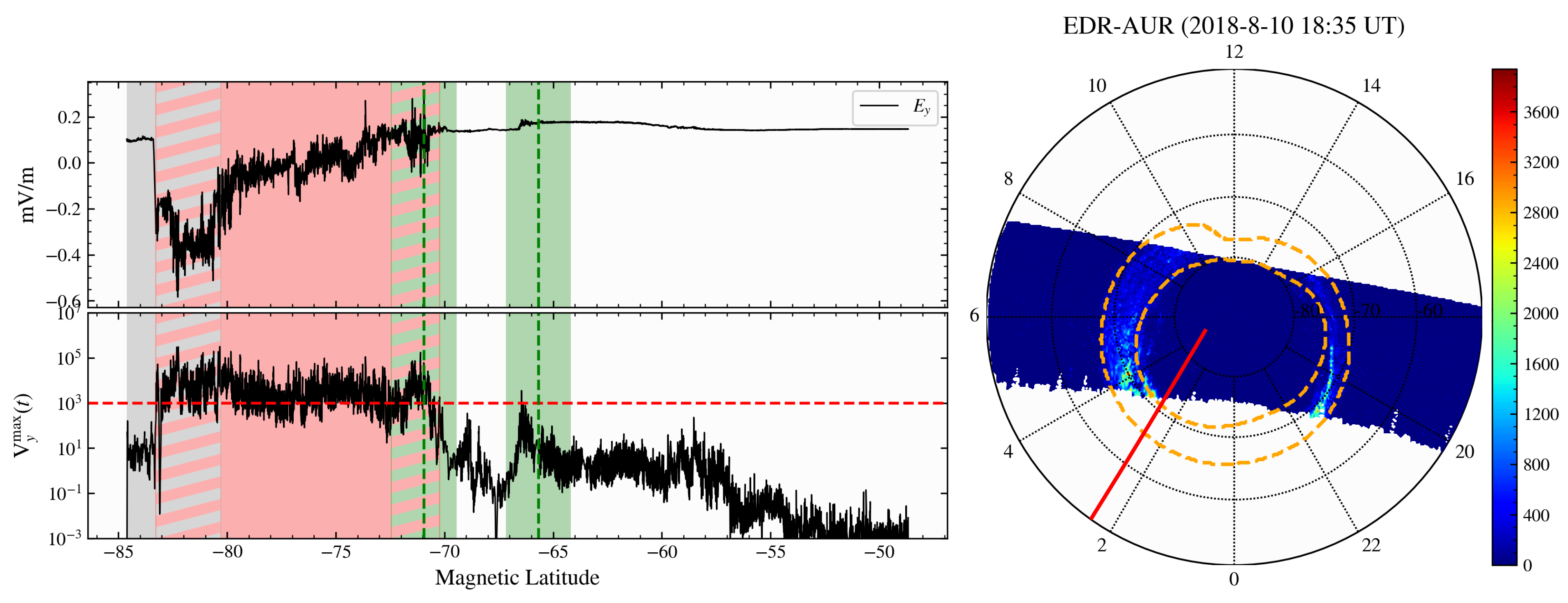
| 2881 [S] | night | 10 August 2018 18:49:57 ÷ 18:59:23 | −84.61/−48.67 | 1 | 80 |
| 2888 [S] | night | 11 August 2018 05:53:06 ÷ 06:02:32 | −59.08/−30.35 | 2 | 220 |
| 2898 [N] | day | 11 August 2018 20:53:04 ÷ 21:02:29 | +78.83/+46.18 | 2 | 250 |
| 2898 [S] | night | 11 August 2018 21:40:29 ÷ 21:49:54 | −78.42/−46.78 | 4 | 550 |
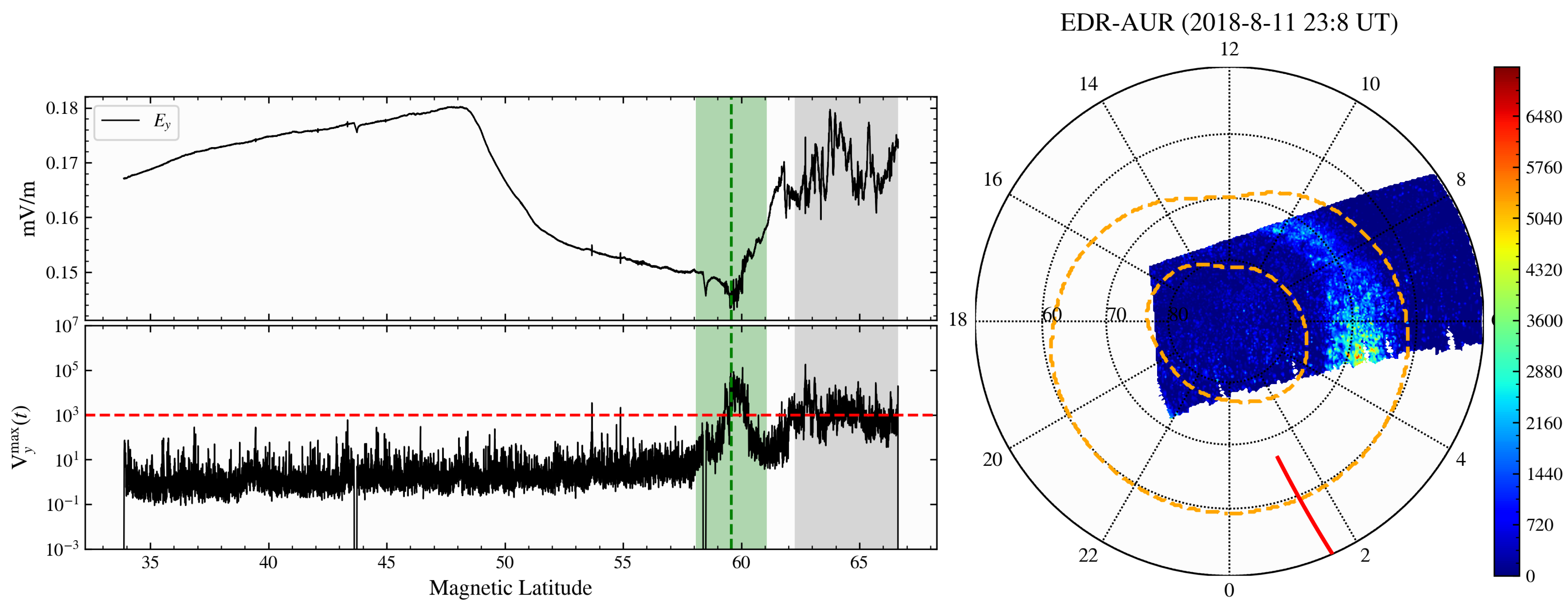
| 2898 [N] | night | 11 August 2018 22:08:21 ÷ 22:17:35 | +33.88/+66.63 | 4 | 850 |
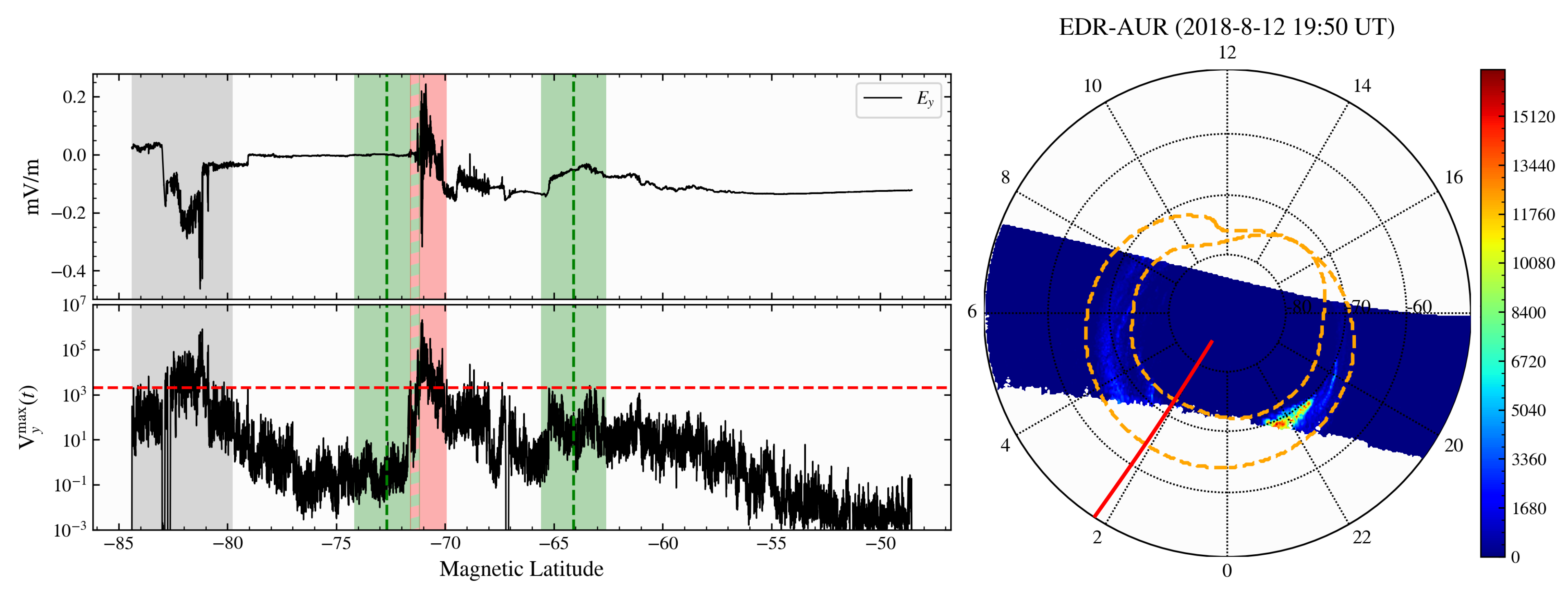
| 2912 [S] | night | 12 August 2018 19:46:46 ÷ 19:56:13 | −84.40/−48.55 | 2 | 100 |
| 3122 [N] | night | 26 August 2018 15:49:09 ÷ 15:58:22 | +31.81/+64.82 | 6 | 750 |
| 5060 [S] | day | 1 January 2019 02:58:46 ÷ 03:06:51 | −45.44/−77.18 | 1 | <50 |
| 7243 [S] | night | 24 May 2019 18:04:30 ÷ 18:12:37 | −79.24/−48.50 | 2 | 50 |
| 8589 [S] | day | 21 August 2019 07:01:23 ÷ 07:09:30 | −48.59/−74.99 | 1 | 80 |
| 9095 [S] | night | 23 August 2019 14:17:13 ÷ 14:25:18 | −67.48/−42.67 | 1 | <50 |
| OrbitNum [N/S] | Side | AOD Result | Reason | Figure |
|---|---|---|---|---|
| 2898 [S] | night | TP | - | Figure 5 |
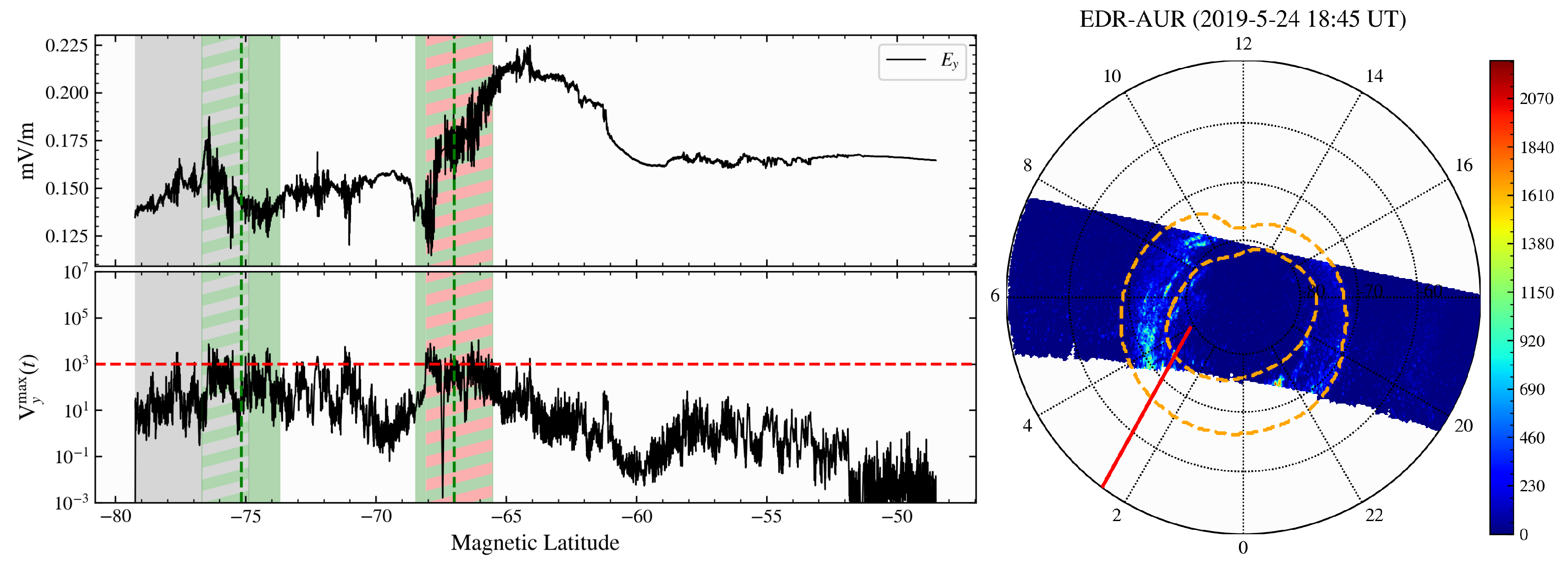
| 7243 [S] | night | TP | - | Figure 7 |
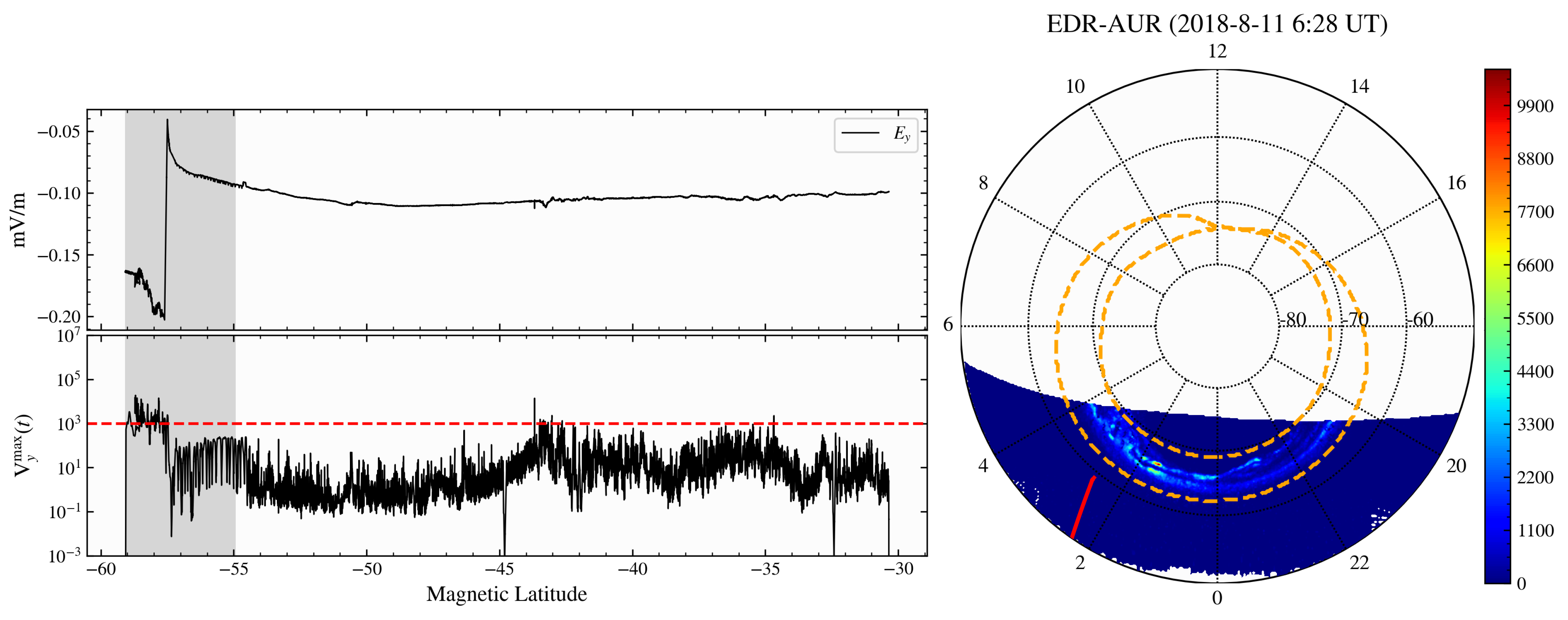
| 2888 [S] | night | TN | - | Figure 8 |
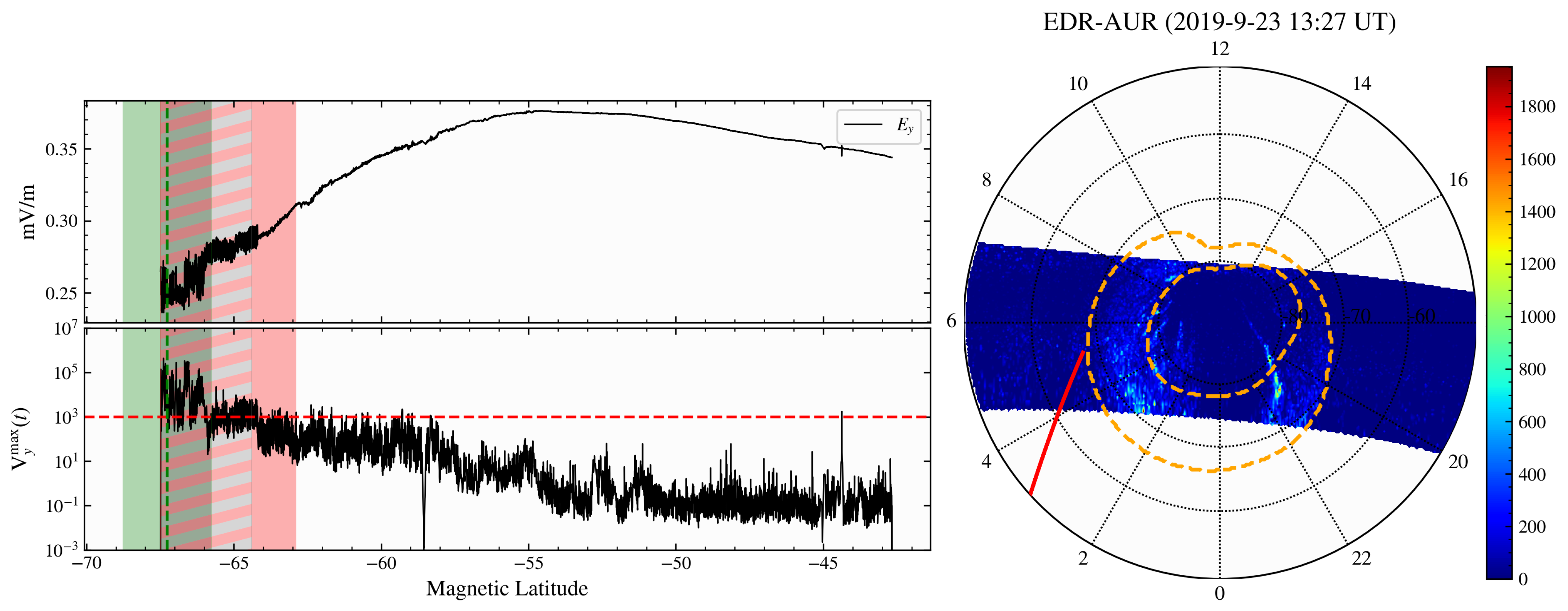
| 9095 [S] | night | FP | spurious effects from electronics switching-on | Figure 9 |
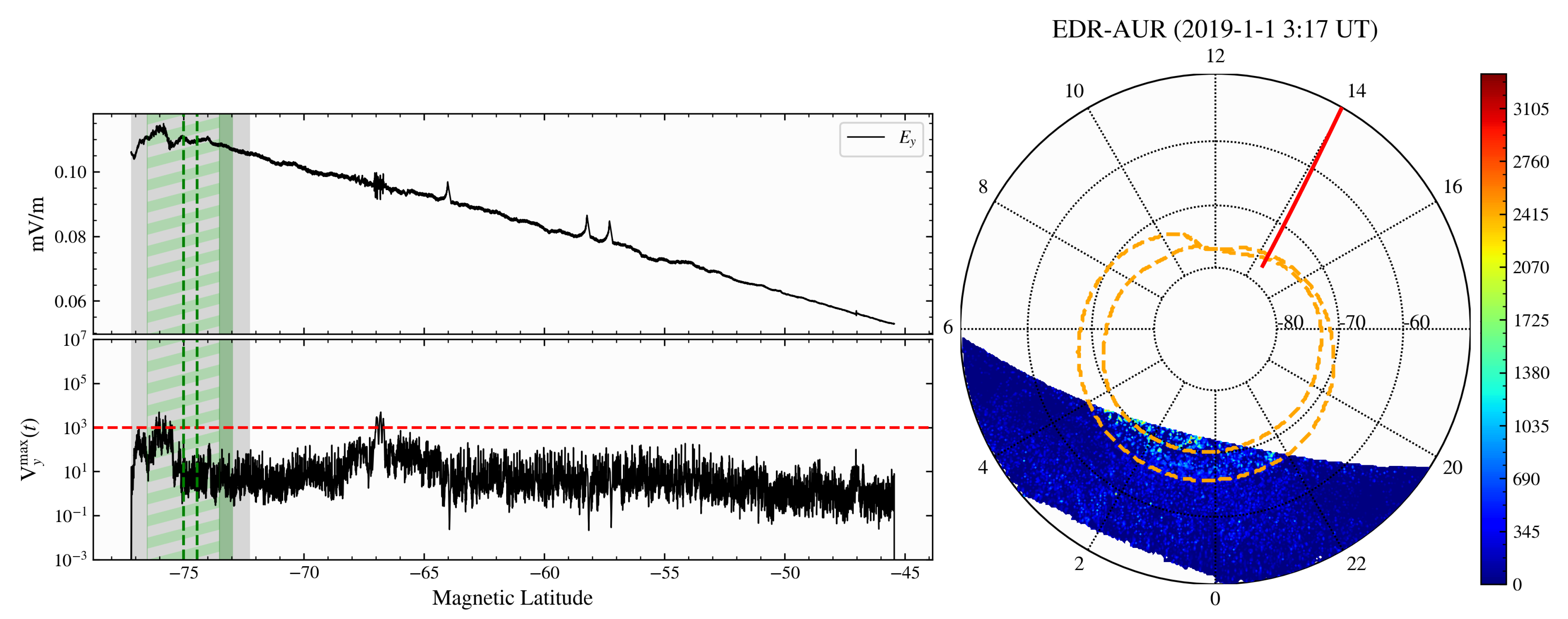
| 5060 [S] | day | TN | - | Figure 10 |
| 8589 [S] | day | FP | activity interval detected at low latitudes | Figure 11 |
| 2898 [N] | day | TP | - | Figure 12 |
| 2898 [N] | night | FN | too short latitudinal interval of activity | Figure 13 |
| 3122 [N] | night | FN | too low activity levels | Figure 14 |
| 2881 [S] | night | SP | polar cap activity detected | Figure 15 |
| 2912 [S] | night | TP | positive detection with quiet polar cap | Figure 16 |
Disclaimer/Publisher’s Note: The statements, opinions and data contained in all publications are solely those of the individual author(s) and contributor(s) and not of MDPI and/or the editor(s). MDPI and/or the editor(s) disclaim responsibility for any injury to people or property resulting from any ideas, methods, instructions or products referred to in the content. |
© 2023 by the authors. Licensee MDPI, Basel, Switzerland. This article is an open access article distributed under the terms and conditions of the Creative Commons Attribution (CC BY) license (https://creativecommons.org/licenses/by/4.0/).
Share and Cite
Papini, E.; Piersanti, M.; D’Angelo, G.; Cicone, A.; Bertello, I.; Parmentier, A.; Diego, P.; Ubertini, P.; Consolini, G.; Zhima, Z. Detecting the Auroral Oval through CSES-01 Electric Field Measurements in the Ionosphere. Remote Sens. 2023, 15, 1568. https://doi.org/10.3390/rs15061568
Papini E, Piersanti M, D’Angelo G, Cicone A, Bertello I, Parmentier A, Diego P, Ubertini P, Consolini G, Zhima Z. Detecting the Auroral Oval through CSES-01 Electric Field Measurements in the Ionosphere. Remote Sensing. 2023; 15(6):1568. https://doi.org/10.3390/rs15061568
Chicago/Turabian StylePapini, Emanuele, Mirko Piersanti, Giulia D’Angelo, Antonio Cicone, Igor Bertello, Alexandra Parmentier, Piero Diego, Pietro Ubertini, Giuseppe Consolini, and Zeren Zhima. 2023. "Detecting the Auroral Oval through CSES-01 Electric Field Measurements in the Ionosphere" Remote Sensing 15, no. 6: 1568. https://doi.org/10.3390/rs15061568