Article

Synthetic Aperture Radar Monitoring of Snow in a Reindeer-Grazing Landscape

1
Department of Physical Geography, Stockholm University, 106 91 Stockholm, Sweden
2
Bolin Centre, Stockholm University, 106 91 Stockholm, Sweden
*
Author to whom correspondence should be addressed.
Remote Sens. 2024, 16(13), 2329; https://doi.org/10.3390/rs16132329
Submission received: 25 March 2024 / Revised: 14 June 2024 / Accepted: 21 June 2024 / Published: 26 June 2024
(This article belongs to the Section Ecological Remote Sensing)

Abstract

:
Snow cover and runoff play an important role in the Arctic environment, which is increasingly affected by climate change. Over the past 30 years, winter temperatures in northern Sweden have risen by 2 °C, accompanied by an increase in precipitation. This has led to a higher incidence of thaw–freeze and rain-on-snow events. Snow properties, such as the snow depth and longevity, and the timing of snowmelt in spring significantly impact the alpine tundra vegetation. The emergent vegetation at the edge of the snow patches during spring and summer constitutes an essential nutrient supply for reindeer. We have used Sentinel-1 synthetic aperture radar (SAR) to determine the onset of the surface melt and the end of the snow cover in the core reindeer grazing area of the Laevás Sámi reindeer-herding community in northern Sweden. Using SAR data from March to August during the period 2017 to 2021, the start of the surface melt is identified by detecting the season’s backscatter minimum. The end of the snow cover is determined using a threshold approach. A comparison between the results of the analysis of the end of the snow cover from Sentinel-1 and in situ measurements, for the years 2017 to 2020, derived from an automatic weather station located in Laevásvággi reveals a 2- to 10-day difference in the snow-free ground conditions, which indicates that the method can be used to investigate when the ground is free of snow. VH data are preferred to VV data due to the former’s lower sensitivity to temporary wetting events. The outcomes from the season backscatter minimum demonstrate a distinct 25-day difference in the start of the runoff between the 5 investigated years. The backscatter minimum and threshold-based method used here serves as a valuable complement to global snowmelt monitoring.

1. Introduction

Arctic environments are experiencing increasing temperatures at a rate that is about twice as fast as the average rate for the rest of the world [1]. The most pronounced increase has occurred during the winter and spring seasons [2,3,4]. In northern Sweden, the average winter temperatures exhibit a 2 °C increase over the past 30 years [5]. Warming scenarios also indicate a rise in winter snow accumulation, along with notable changes in the snow properties [6]. A changing winter climate has serious implications for reindeer husbandry in northern Scandinavia. Higher winter temperatures lead to more frequent occurrences of temperature fluctuations above and below zero, rain-on-snow events and thaw–freeze cycles [7,8]. Rain-on-snow involves melting and subsequent refreezing, creating hard layers at the base or within the snowpack, which make grazing difficult [8]. These types of events can also create conditions favourable for mould, resulting in toxic lichens [5] and adversely affecting the nutrient-holding capacity of Carex bigelowii [9]. Unfortunately, the frequency of such events is predicted to increase with further warming [3,8].
Plants adapted to low temperature and low nutrient supply, frost tolerance and photosynthetic efficiency characterise the alpine tundra vegetation. The most critical parameters affecting the length of the growing season in alpine tundra ecosystems are the snow accumulation during the winter [10,11], snowmelt timing [12], soil temperature beneath the snowpack, and air temperature before, during and after snowmelt [7,13,14]. Consequently, even a slight alteration in the length of the spring season by just a few weeks can have a substantial impact on these complex arctic systems [12,14,15]. Furthermore, snow-covered ground contains relatively higher soil nutrient content, and therefore, shorter snow seasons with reduced snow cover may adversely impact soil nutrients [10,16,17]. Previous studies have shown that the distribution of alpine tundra vegetation is strongly related to the snowmelt gradient [18,19]. The altered snow conditions resulting from rising temperatures and changing precipitation patterns [20] make it challenging for reindeer to smell, identify, and access the ground lichens they feed upon during winter [5].
Reindeer move over large distances during their annual cycle and use different habitats during winter, spring, summer and autumn grazing [5,21]. Grazing modifies the vegetation above and below ground [22]. A change in the grazing pattern can lead to a loss of plant biodiversity in the area [23] and lead to the ecosystem transitioning from moss-shrub-dominated tundra to graminoid-dominated tundra [24]. It has been suggested by Cohen et al. [25] that reindeer grazing may reduce ground heating because the grazing reduces the height of the vegetation, which, in turn, prolongs the snow cover and increases the albedo, thereby extending the spring snowmelt. In the alpine landscape, reindeer selectively forage in response to snowmelt gradients, often favouring snow-bed meadows with high plant diversity [26]. The prime period of nutritional abundance in vegetation aligns with the early stages of the growing season [27]. The improved nutrient quality during spring and early summer is crucial for the growth of both adult reindeer and calves. A later start to the growing season can substantially impact calf growth [5,28].
There is a significant variation in the types of forage consumed by reindeer throughout the year [29]. In spring, reindeer in Fennoscandia tundra ecosystems primarily consume 62% lichen, for example, Cladonia, 8% shrub, Betula nana, and 12% graminoids, including Deschampsia flexuosa and Carex Bigelowii [30]. During summer, the shrub and graminoid intake increases to 29% and 23%, respectively, with a decrease in lichen consumption [30]. One effect of higher summer temperatures is an increased number of insects, which can, in turn, cause stress in reindeer and make them migrate to higher altitudes, where food resources are more limited [5,31]. However, during warm summer days, reindeer prefer grazing on fresh vegetation appearing at the rim of the high-altitude perennial and seasonal snow patches. Due to the warming, this food resource is also diminishing [25,32]. The spring snowmelt season is an essential component of the arctic environments; remote sensing is an efficient way to monitor changes in high latitudes [33].
Active microwave synthetic aperture radar (SAR) enables all-weather day and night imaging. Sentinel-1 (S-1) SAR offers a 6-day revisit time at the equator, with 2 satellites in a 12-day orbit and a spatial resolution of around 20 m before speckle filtering [34]. Previous studies have used the SAR backscatter coefficient to measure the snowmelt and to generate snow cover maps [35,36,37], monitor snow wetness [38] and assess the relationship between the spring snowmelt and tundra vegetation changes [17,39].
Dry snow conditions generally result in higher backscatter than wet snow conditions due to the lower absorption and higher scattering at the snow–ground interface. In spring, there occurs a period of alternating low and high backscatter as the snow begins to accommodate more liquid, and then, during the ripening phase, the backscattering values start to steadily decrease (Figure 1). The season minimum of the S-1 backscatter determines the start of the surface melt (SOSMS-1). In this study, the SOSMS-1 is employed to delineate the transition from dry snow to a snowpack with persistent liquid water during daytime. The S-1 end of the snow cover (EOSS-1) is when the backscatter reaches its highest value after the SOSMS-1 [36].
The objective of this study is to determine if the timing and spatial distribution of the snowmelt in the Laevás Sámi reindeer-herding area during the period 2017 to 2021 can be derived from S-1 SAR data. The choice of years is based on the availability of satellite data and in situ data from an automatic weather station (AWS) located in Laevásvággi [5,40]. In this study, we establish the beginning and end of the snowmelt period during the spring and summer season (March–August) using Sentinel-1 SAR data over the Laevás reindeer-herding area. We investigate the snowmelt timing and distribution linked to alpine vegetation important for reindeer grazing.

2. Study Area and Datasets

2.1. Study Area

The area of interest (Figure 2) is the western part of the Laevás Sámi reindeer-herding area (18.5E°, 68.5N°) where, traditionally, the spring and summer grazing occurs [5,41]. It is located in a sub-arctic environment in Kiruna municipality in northern Sweden. The area is located along a west–east oceanic–continental climate gradient with a rain shadow effect from the highest part of the Scandinavian mountain range [5]. Covering an expanse of 1038 km2, this diverse area is alpine, with altitudes up to 2003 m.a.s.l dominated by heath and bare surfaces. Valleys are forested with Betula pubescens ssp. Czerepanovii [42]. Lush meadow vegetation covers the mountain slopes, and in the wind-exposed heath, dwarf shrubs and lichens grow sparsely on the gravelly substrate [43]. Laevásvággi, which is a core area because reindeer calve there in the spring [5], is located between Rávttasjávri and Visttasvággi and the vegetation there is dominated by extremely wind-exposed heath and grasslands with grasses and herbs including D. flexuosa and C. Bigelowii and dwarf shrubs, for example, B. nana [42].

2.2. Datasets

We used single-look complex (SLC) S-1 SAR data in interferometric wide-swath mode (IW) in the VV and VH polarisations. The acquisitions were from the 1st of March to the 30th of August from 2017, 2018, 2019, 2020 and 2021 in the ascending relative orbit 131, except for the 4th of July 2021, which has orbit 58, downloaded from the Alaska Satellite Facility [45] with a repeat cycle of six days, except for the 27th of June to 9th of July, where there was no acquisition on the 2nd of July over the area of interest. All the images were acquired around 4:15 pm UTC. In total, we used 31 scenes from 2017, 35 scenes from 2018, 33 scenes from 2019, 36 scenes from 2020, and 37 scenes from 2021 (Figure 3). Additionally, a digital elevation model (DEM) with a spatial resolution of 2 m, provided by Lantmäteriet [44], was used to pre-process and radiometrically normalise the S-1 scenes. Data from an automatic weather station (AWS) were provided by Rosqvist et al. [5] and the Swedish Infrastructure for Ecosystem Science [40] for the years 2017 to 2020. The AWS collected the average, minimum, and maximum daily air temperature, snow depth and rainfall at a location in Laevásvággi. The snowmelt patterns were compared with landcover data provided by Lantmäteriet [43].

3. Method

3.1. Pre-Processing of Sentinel-1 Data

A temporal stack of backscatter coefficient (γ0) intensities in dB was generated for both polarisations (VV and VH) [36]. All the scenes were pre-processed using graph builder and bulk processing in the European Space Agency Sentinel Application Platform (SNAP) version 8.0.9 (Figure 4). Automation using Python 3.9 was performed in PyCharm 2022.1.1. The data were pre-processed with the latest orbit file containing the satellite position, velocity, and orientation information over time [36]. The image’s swaths were then split, deburst and merged between the sub-swaths IW2 and IW3 into a single image. Next, a subset of the area was extracted using the coordinates for the study area mentioned earlier (Section 2.1). The next step involved calibration of the backscatter coefficient or beta-nought (β0), which measures the radar signal reflected from the Earth’s surface back to the satellite. The data underwent terrain-flattening correction using the 2 m DEM from Lantmäteriet [44]. This involved estimating a reference surface [44] to correct for roughness [46,47] and rectify each pixel’s location, brightness, and radiometry [46], as well as to correct for atmospheric absorption [47]. The processed data were multilooked with 4 azimuth and 1 range samples; a 5 × 5 Lee Sigma speckle filtering with a sigma value of 0.9 was then applied [36,48]. Geometric terrain correction was applied to translate each input data product separately and convert the SAR to map geometry. Precise external orbital state vectors were utilized to interpolate each azimuth line in the application of range-Doppler geolocation [47]. The backscatter measurements were then resampled from the slant or ground range geometry of the input products into the map geometry of the national elevation model, which was provided Lantmäteriet [44]. All the scenes were resampled to 15 × 15 m, and radiometric layover and shadow pixels were excluded.

3.2. Extracting SOSM and EOS Using Python

Using Python, the SOSM and EOS were extracted from the stacks of pre-processed S-1 images from all five years, and both polarisations were extracted following Buchelt et al. [36]. Processing scripts were rewritten for this project to reduce the processing time and provide a better overview of the processing of the S-1 images. The NumPy 1.22.4 library was utilized in all the matrix calculations to speed up the heavy data processing. The Geospatial Data Abstraction Library (GDAL) 3.4.3 was used for the input and output operations, resampling, and accessing metadata.
First, the SOSMS-1 in each pixel was identified and the day of year (DOY) recorded (Equation (1)). For each pixel in the image stack along the time axis, the function computes the minimum value of the backscatter intensity (γ0), which corresponds to the earliest date when snowmelt occurred for that pixel. Pixels with missing data were assigned a “no data” value. The SOSMS-1 phase detection was defined from Buchelt et al. [36]:
S O S M S - 1 x ,   y = D O Y , i f   γ 0 x ,   y ,   D O Y = min ( γ 0 )                                                               1 ,   o t h e r w i s e .
After that, the EOSS-1 was determined for the threshold (Equation (2)), while the DOY of the EOSS-1 was determined when the backscatter had passed two criteria [36]. First, it had to exceed the chosen threshold in three consecutive images; the threshold was established based on the typical seasonal backscatter behaviour [49]. The main threshold in this study was 3 dB, but for comparison, a threshold of 4 dB was also implemented for all the images. In order to detect possible refreeze and re-melt, a second criterion, a re-melt threshold, was employed. The threshold needed to exceed the season minimum by more than the chosen threshold and to be continued in at least three images to pass the re-melt threshold. The second criterion was applied to prevent false backscatter detection caused by melt and refreeze. The threshold-based EOSS-1 approach detected the point at which a pixel’s backscatter intensity (γ0) exceeded the season minimum and the threshold (t) [36]. The EOSS-1 were defined as [36]:
E O S S - 1 x , y = f i r s t   D O Y ,                                                 w h e r e   γ 0 ( x ,   y D O Y )                                                                                     > min γ 0 + t                                                                 ( t h r e e   c o n s e c u t i v e   t i m e s ) s t a r t o f s e a s o n   s n o w   f r e e   ,             o t h e r w i s e .
Equation (2) identifies the minimum value for each pixel in the stack. Then, for each day afterwards in the stack, the t was applied to check if the snowmelt has stopped. If the snowmelt had stopped, the day of the year for EOSS-1 was determined, and pixels where the threshold is not reached were assigned “no data” values [36].
For the year 2017 to 2020, the EOS from S-1 was compared to in situ data from Laevásvággi AWS [5,40] by comparing the value of the pixel nearest to the Laevásvággi AWS located at 18.96°E 68.04°N. The nearest pixels in the EOSS-1 and Laevásvággi AWS for four years are shown in Section 4.3. Finally, for the extracted SOSMS-1 and EOSS-1, raster zonal statistics were calculated for mountain vegetation data provided by Lantmäteriet [43] using ArcGIS Pro 2.9.5.

4. Results

4.1. Backscatter Behaviour between the Different Polarisations and Years

There is a distinct difference between the years in terms of the backscatter behaviour between during the spring and summer season (March–August). The moistening and ripening phase started later in 2017 and 2020 than in 2018 and 2019, indicating a difference in the longevity of the snow cover. The average overall backscatter intensity at the seasonal minimum in 2017 and 2020 was lower than in 2018 and 2019 in both polarisations, though the difference in VH is close to the reported radiometric accuracy [50]. An exception is 2021, which shows a much lower backscatter on day 136 (16/5) compared to previous years in both polarisations. The S-1 backscatter trend in both polarisations over 5 years is characterized by a period of prolonged high backscatter intensity of between 30 and 36 days before it reaches the ripening phase (Figure 5). However, in 2017, the VV polarisation exhibited lower backscatter intensity between DOY 73 (14/3) and DOY 85 (26/3) before returning to the previous level. The VV polarisation has a higher intensity than the VH, but the VV intensity exhibits a larger range between the highest and lowest values.

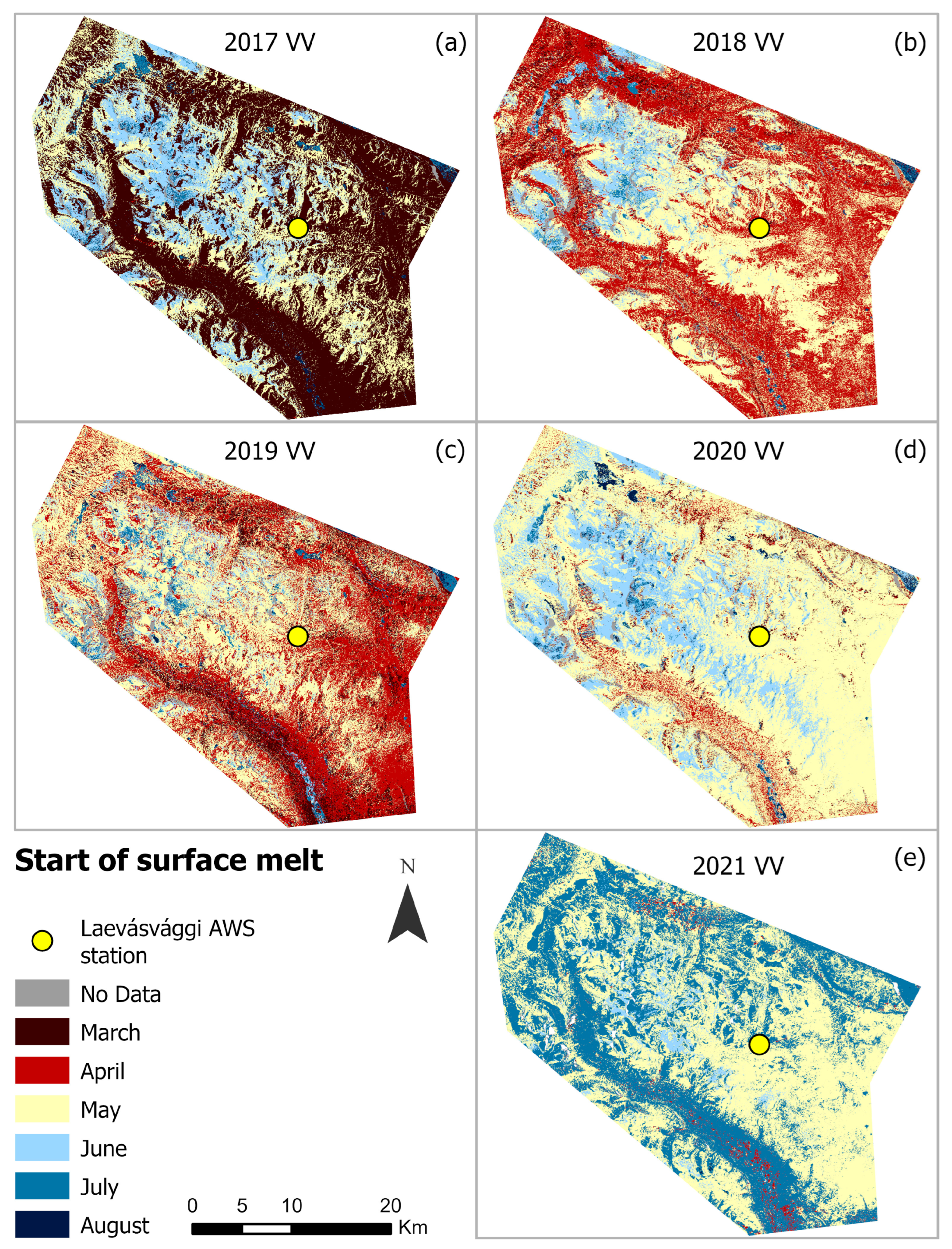
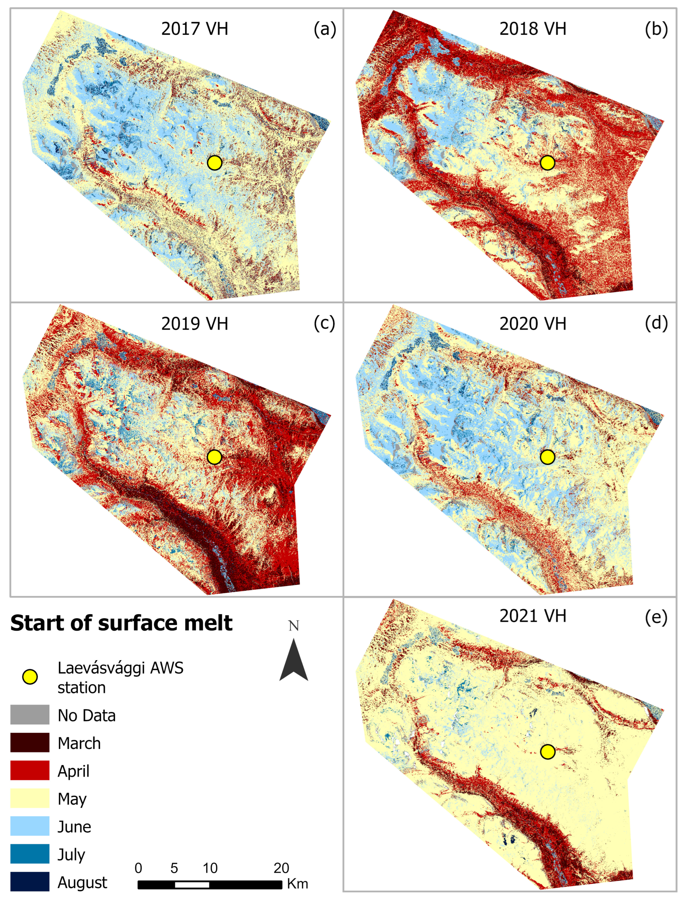
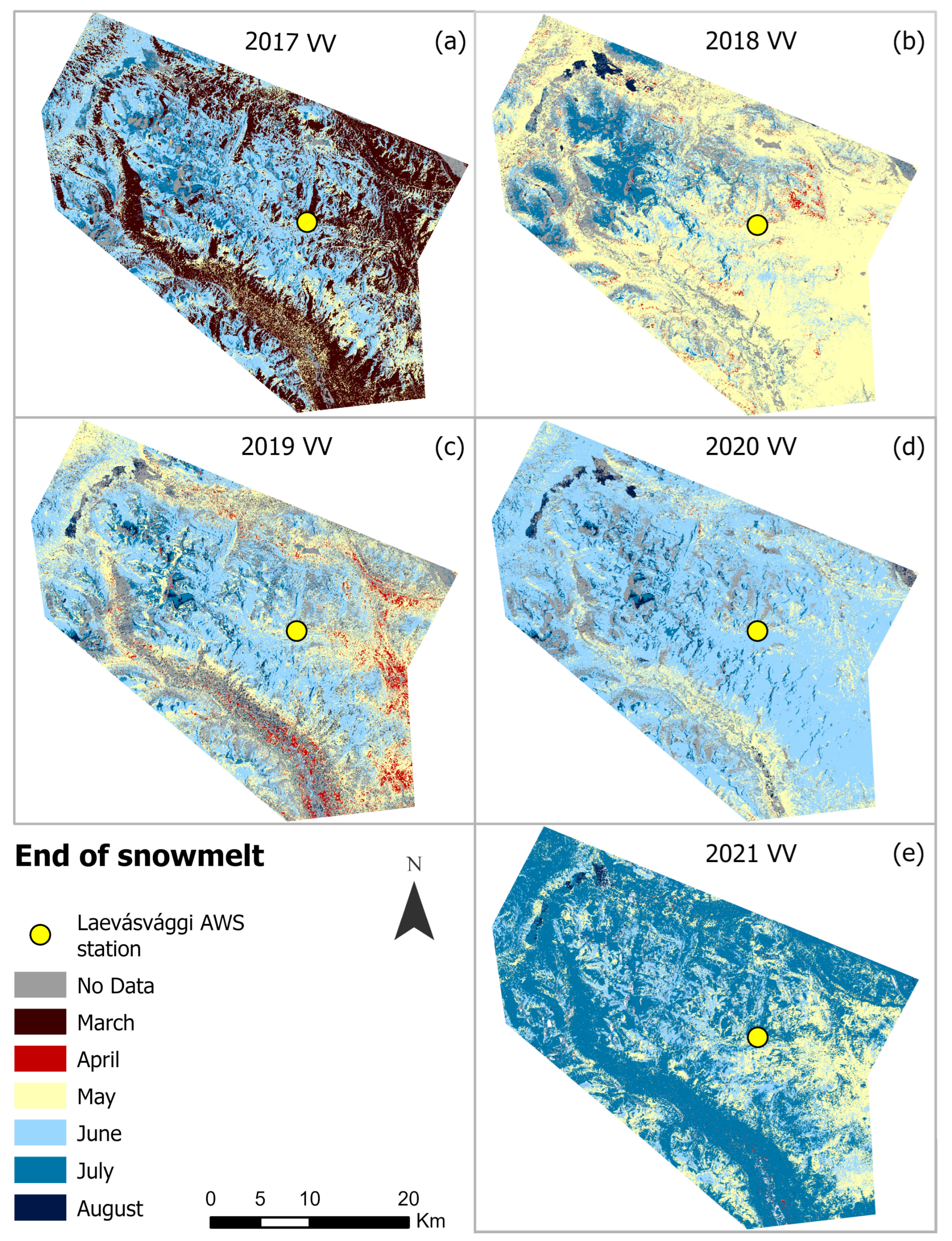
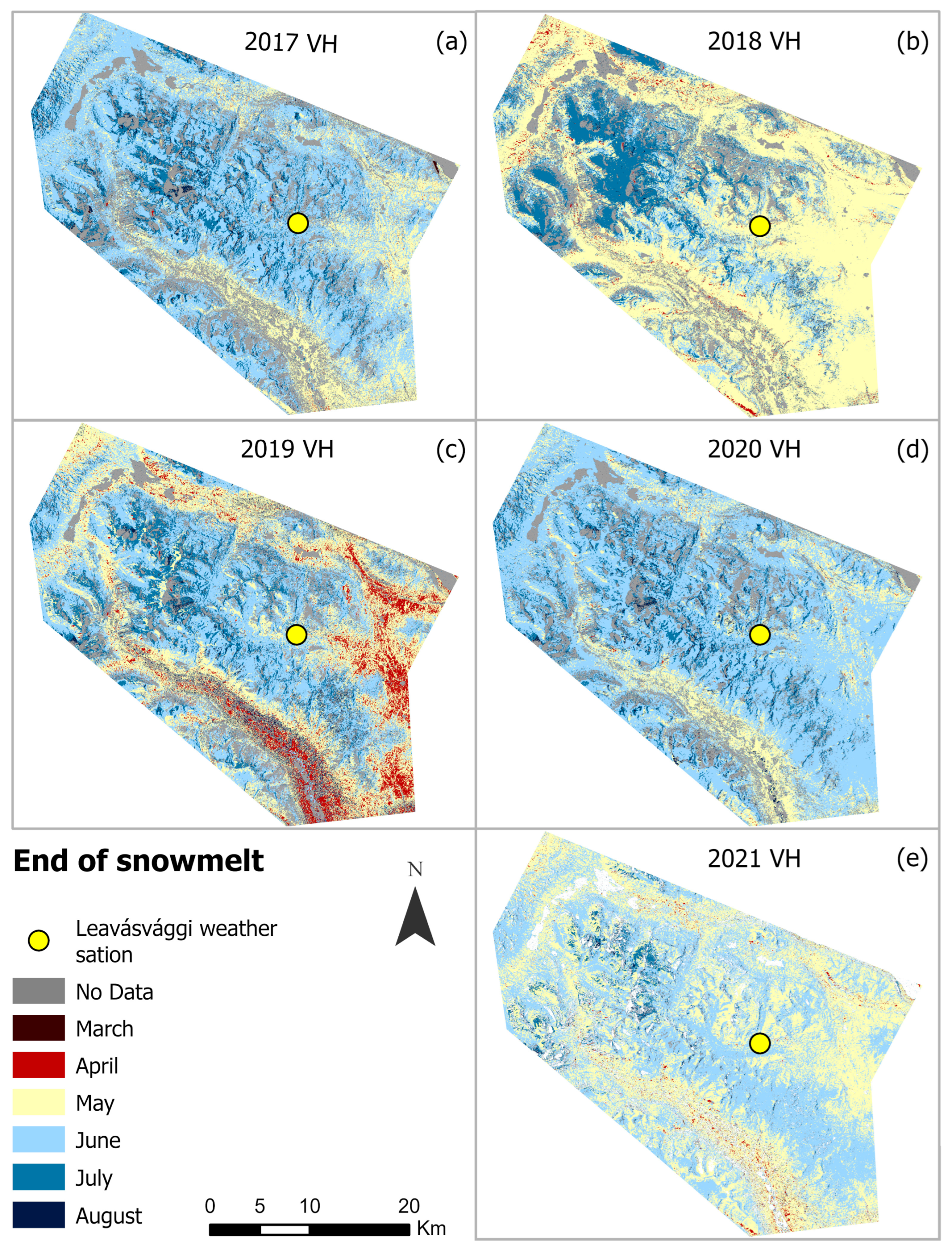
4.2. Seasonal Variations in SOSM and EOS from Sentinel-1 (2017–2021)

The analysis of the S-1 data shows that the snowmelt in the study area differs between the years 2017 and 2021 (Figure 5). The ripening phase, when the backscatter curve has a downward trend before reaching the minimum seasonal backscatter coefficient, differs across all the years, with a span of approximately 25 to 45 days. The date of the minimum backscatter (SOSMS-1) is also different between years. The minimum backscatter occurs at day 151 (31/5) in 2017, day 154 (2/6) in 2020 and day 136 (16/5) in 2021, and about 25 days earlier in 2018 and 2019, at day 122 (2/5) and day 123 (3/5). This indicates that the spring snow-melting period, after the backscatter has reached its minimum values, started about 25 days earlier in 2018 and 2019 than in 2017 and 2020.
In 2017, the greatest number of pixels identified as the SOSMS-1 was observed at day 79 (20 March) in the VV (56% of the area), which was not found in the VH or other years (Table 1 or Figure 6a). Instead, the VH for the same year showed large SOSMS-1 areas in May (25%) and June (15%) rather than in March (Figure 7b). In 2018 and 2019 (Figure 6b,c, and Figure 7b,c), both polarisations showed similar patterns of the SOSMS-1, with some variations in different slopes and elevations. The analysis identified the highest amount of SOSMS-1 in 2018 in April (46% in VV and 39% in VH) and May (37% VV and VH). In 2019, the largest number of pixels identified as the SOSMS-1 was in April (39% in VV and 35% in VH) and May (37% VV and 36% VH). In 2020 (Figure 6d and Figure 7d), the VV showed the largest SOSMS-1 in May (65%) and June (20%), while the VH showed a more even SOSMS-1 throughout May (50%) and June (28%). In 2021, both the VV and VH exhibited an SOSMS-1 in May, with the VV at 62% and VH at 96%. However, while the VV showed a significant snowmelt in July (53%), the VH exhibited its peak only in May (Figure 6e and Figure 7e). There is a similarity in the SOSMS-1 patterns in 2017 (VH) and 2020 (VV and VH) and between the years 2018 (VV and VH) and 2019 (VV and VH). The results show the delayed onset of the spring surface melt in 2017 and 2020 compared to 2018 and 2019. After the backscatter minimum, the runoff phase differs in length between the polarisations in 2019 by 18 days between the VV and VH but is similar in both polarisations in the other years, with a range of 49 to 107 days. The EOS occurs at day 211 (30/7) in 2017 and day 212 (31/7) in 2018, at day 207 (26/7) in the VH and day 237 (25/8) in the VV in 2019, day 214 (1/8) in 2020 and day 185 (4/7) in 2021. In 2021, the runoff period was the shortest compared to previous years, lasting only 49 days.
From 2017 to 2021, the Laevás reindeer-grazing region experienced significant changes in the EOSS-1, according to the data (Figure 8 and Figure 9). The EOSS-1 was identified for all the years, and in 2017 (Figure 8a and Figure 9a), there was a clear difference between the polarisations. The VV had a higher number of pixels identified as the EOSS-1 in March (40%), while a larger EOSS-1 was observed in June for the VH (49%) but also for the VV (38%). The highest amount of the area that was identified as the EOSS-1 for 2018 (Figure 8b and Figure 9b) was found in May (54%), and for 2019 (Figure 8c,e and Figure 9c), the EOSS-1 was similar in both polarisations, with the highest number of pixels in May (30% in VV and 28% in VH) and June (34% in VV and 31% in VV). There was an equivalency in the EOSS-1 in 2020 (Figure 8d and Figure 9d) for both polarisations, with the highest number in June (66% for VV and 56% for VH). In 2021, both the VV and VH exhibited an EOS in May (VV at 24% and VH at 48%). However, while the VV showed a significant snowmelt in July (77%), the VH exhibited an EOS in June (53%).

4.3. Sentinel-1 and In Situ Data from Laevásvággi AWS

The comparison of the EOSS-1 and ground data collected by the Laevásvággi AWS [5,40] revealed a difference of 2 to 10 days between the timing of the EOSS-1 and the in situ measurements (Table 2). However, anomalies were detected in 2019, where the EOSS-1 indicated a delay to 7 and 13 August, which is beyond the expected range. In all the years except for 2019, the day the ground becomes snow-free is consistent across both polarisations. It should be noted that the S-1 method, requiring 3 consecutive acquisitions, introduces a potential lag of up to 12 days in the estimates of the SOSM and EOS. Comparisons with in situ data should take this into consideration.

4.4. Differences between Landcover Classes

The zonal statistics were extracted from the SOSMS-1 and EOSS-1 datasets (VV and VH and all years) for different landcover classes. The resulting statistics, including the mean DOY values and the standard deviation (STD) per class, represent the degree of variation or spread around the mean DOY value in the different types of vegetation. These statistics are presented in Table 3 for SOSMS-1 and Table 4 for EOSS-1.
The results reveal notable variations across the vegetation classes, polarisations, and years. As mentioned earlier, the VV data from 2017 show an anomaly compared to the VH data from the same year and other investigated years. For example, in 2017, dry heath and alpine low grass meadow exhibited the SOSMS-1 around day 98 and 103 (VV), respectively, compared to approximately day 125 and 134, respectively, for the VH polarisation (Table 3). In 2020, dry heath and alpine low grass meadow showed the SOSMS-1 at day 112 and 119 (VV), respectively, contrasting with approximately day 108 and 115, respectively, for the VH polarisation. In 2021, the mean DOY for the SOSMS-1 in alpine low grass meadows was observed at day 158 for the VV and day 134 for the VH. In dry heat, the mean DOY was day 161 for the VV and day 128 for the VH. Notably, there was a 26-day difference observed within specific landcover classes in the VV and a 21-day difference in the VH.
Furthermore, between the VV data from 2018 and 2019, there is a 1- to 12-day difference in the timing of the SOSMS-1 within specific landcover class. Similarly, the difference between the VH data from 2018 and 2019 ranges from 3 to 14 days.
The study area primarily consists of two dominant landcover classes: dry heath and alpine low-grass meadow. The range of variation in the start of the SOSMS-1 each year across the different landcover class extends from a minimum of 10 days in 2020 to a maximum of 29 days in 2019. Laevásvággi exhibits three main landcover classes: dry heath, extreme dry heath, and alpine low-grass meadow. The time difference in the mean DOY between 2018 and 2019 is only seven days in both polarisations for all three landcover classes. However, in 2020, and specifically in 2021, the SOSMS-1 occurred later in all three landcover classes compared to previous years.
The most significant variation is observed in the mean DOY in the EOSS-1 for grassland vegetation between 2017 and the subsequent years for both the VV and VH polarisations (Table 4). Specifically, in 2017, the mean EOSS-1 date for the VV polarisation was approximately day 133, contrasting with approximately day 114 for the VH polarisation, while in 2020, these dates shifted to around day 145 (VV) and day 133 (VH), respectively. In 2021, there was a later overall mean DOY for the EOSS-1. The mean DOY across different vegetation classes and polarisations ranged from day 136 to day 191, indicating a delayed EOSS-1 compared to previous years.

5. Discussion

The goal of this investigation was to determine if information about the timing and spatial distribution of snowmelt in the Laevás Sámi reindeer-herding area can be derived from Sentinel-1 SAR data between the years 2017 and 2021. The results from Sentinel-1 showed that there was high variability between the years in the timing of the start of the snowmelt, which began 25 days earlier in 2018 and 2019 compared to 2017 and 2020.

5.1. Variation in Backscattering and Spring Snowmelt

There was similar backscatter behaviour over time for each of the five years (2017−2021). Also, the three melting phases defining the snow melting process, moistening, ripening, and runoff, can be distinguished using multi-temporal C-band SAR measurements in the study area. These results compare well with the findings of Buchelt et al., Marin et al. and Lund et al. [36,49,51].
It is notable that there are significant differences in elevation across the study area, which may explain the early SOSM across the valleys in 2017. The difference in the VV and VH responses in March 2017 is difficult to explain. The VV backscatter recovered after dipping to −11 dB, which may indicate that VH data provide a more stable response to short-term weather events (Figure 5). The onset of melt, particularly at lower elevations, may also indicate warm air intrusion in the valleys that caused some wetting of the snow surface to which the co-polarised channel was more sensitive, perhaps due to volume scattering from shrubs and trees in the cross-polarised data (Figure 6, Figure 7, Figure 8 and Figure 9). Spring 2017 otherwise experienced deep snow late into the spring, according to data from the Swedish Meteorological and Hydrological Institute [52]. The results from 2021 show that the VV signal is confused by the presence of vegetation in the forested lowlands. The sharp contrast in the timing of the SOSMS-1 in the VV and VH strongly argues for the use of VH data where possible. Failing that, we recommend masking out forests and dense shrublands.
All the S-1 SAR data that were used for this study were acquired in the afternoon and can therefore provide an earlier SOSMS-1 because of the natural 24 h cycle of the snowpack, with greater potential for daytime surface melt and refreeze during the night [36]. In Visttasvággi, the vegetation includes taller vegetation such as birches. When the radar encounters elements like tree trunks, leaves, and branches within a forest canopy, it experiences double bounce and volume scattering, typically resulting in higher backscatter [39]. The method used in this paper may be particularly effective for studying the snowmelt in areas without significant tree height variations due to the distinctive values obtained in such an environment. The elevation and terrain significantly influence the environmental conditions that are favourable for the different vegetation habitats’ possibility of establishment within the region. Consequently, the snowmelt pattern varies depending on the dominant vegetation class. Both dry and wet terrain, as well as higher and lower vegetation types, play a decisive role in the rate of snowmelt [53]. Moist–wet heath may impact the S-1 observations due to the greater surface and ground water content affecting the backscatter.

5.2. Impact of Variation in Spring Snowmelt on Vegetation and Reindeer

In the five years of the SOSMS-1 observations, two patterns emerge. Here, 2017 and 2020 show late melting at higher elevations, whereas 2021 shows rapid melting early in the summer. The earlier snowmelt in 2018 might be attributed to an extended period of warm temperatures commencing in May, coupled with lower-than-average precipitation, as indicated by data from the Swedish Meteorological and Hydrological Institute [54]. This high interannual variability will no doubt impact the vegetation productivity [13], with effects on the wildlife [27,29]. Previous investigations indicate that longer growing seasons and the early onset of snowmelt can result in tundra vegetation species being outperformed by species from more temperate biomes [18,55]. Satellite data from 1987 to 2004 show a decline in the number of days with snow cover and an earlier snowmelt in the Northern Hemisphere, with an estimation of 10 to 20% less total snow cover [56] and 4−7 days earlier start of the snowmelt during the time period [56,57]. And since 1990, Sweden has observed a reduction of up to 16 days in the snow-covered season [58]. Prolonged snow-free periods may have detrimental impacts on the environment in these regions, potentially resulting in changed vegetation, for example, shrubification [59], and result in reduced nitrogen levels in deciduous shrub species [55]. Between 1995 and 2011, there was a noticeable increase in the average cover per square meter of both evergreen and deciduous shrubs in the Swedish mountains [60]. Evergreen shrubs, for instance, have risen from 26% to 49% in heath sites, while deciduous shrubs, including B. nana, have increased from 5% to 10%. The expansion of shrubs negatively affects the growth of moss and lichens [60,61]. Longer-term changes with higher air temperature [62] and changes in seasonal snow significantly affect sensitive alpine vegetation [63,64], ultimately affecting grazing opportunities for reindeer.
Changes in the timing of the start of the surface melt impact reindeer as they may miss feeding opportunities, which are crucial for nutrient intake during critical spring and early summer [5,27]. Even small shifts in the snowmelt timing can affect species with an earlier niche, influencing mortality, phenology, and reproduction [65,66,67,68,69]. We detected as much as a 25-day temporal difference between start of the surface melt, which must have impacted the plant communities in the study area significantly [64,70,71].
The five-year study period is too short to provide insights into the long-term impact of changes in the snow cover and surface melt timing on vegetation. However, our results provide information about the large interannual variability of the timing of the snow melt and the length of the snow cover period that is crucial for assessing the impact on plant communities in a changing climate.
As temperatures are predicted to continue to increase in the Arctic, the snow properties and the amount of runoff during spring will be altered in the future. As a result, tundra mountain vegetation will significantly change and the total area covered by tundra will shrink, and the conditions for Laevás reindeer will also change. The method presented here serves as a valuable tool for, for example, decision-makers, applicable in different reindeer husbandry areas, which enables analysis of the impact of the snowmelt on reindeer husbandry.
Therefore, utilization of existing satellite data can provide essential insights into how vegetation is impacted by the reduction of snow patches and the onset of surface melt in northern Sweden. Previous research [36,49,51] underscores the efficacy of backscatter behaviour from synthetic aperture radar (SAR) data as a practical approach for monitoring the Earth’s surface changes. The accessibility of Sentinel-1 data further enhances the feasibility of monitoring the initiation of the surface melt on a national scale.

6. Conclusions

Here, Sentinel-1 SAR data were used to investigate the start of the surface melt and end of the snowmelt from 2017 to 2021 in the spring and summer grazing area of the Laevás reindeer-herding community in northern Sweden. The comparison between the end of the snow melt timing and the snow ground truth data showed promising results, with only a 2- to 10-day time shift, implying that the method is suitable for investigating snowmelt. The results show a clear backscatter behaviour trend for all five investigated years. The result indicates that there was a 25-day difference in the start of the surface melt between the years 2017 and 2020. The snowmelt began earlier in 2018 and 2019 compared to 2017 and 2020, which must have impacted the phenology and hence also reindeer grazing. The unusually early snowmelt detected in the VV data in 2017 suggests that VH data provide a more reliable overview of the SOSM and EOS than VV data. The end of the snow cover occurred at approximately the same time during all five years, which means that the spring and summer seasons were of different lengths between the investigated years. Monitoring the seasonal pattern and changes in snow in the region is essential for assessments of how future climate change will affect reindeers’ ability to find the vital spring and summer food, and it can serve as a valuable supplement for potential climate adaptations.

Author Contributions

Conceptualisation and method: I.C., J.M.W. and G.R.; Data processing: I.C.; Analysis: I.C., J.M.W., G.R. and I.A.B.; Writing: I.C., J.M.W., G.R. and I.A.B.; Supervision: G.R., J.M.W., and I.A.B. All authors have read and agreed to the published version of the manuscript.

Funding

This work was partly funded by the Swedish National Space Agency under grant 178/17.

Data Availability Statement

The data that support the findings of this study are available from the corresponding author, I.C., upon reasonable request.

Acknowledgments

Special thanks to Hampus Carlsson for his invaluable coding assistance, which greatly contributed to this project.

Conflicts of Interest

The authors declare no conflicts of interest.

References

  1. IPCC. Climate Change 2023: Synthesis Report. In A Report of the Intergovernmental Panel on Climate Change. Contribution of Working Groups I, II and III to the Sixth Assessment Report of the Intergovernmental Panel on Climate Change; IPCC: Geneva, Switzerland, 2023; pp. 1–85. [Google Scholar]
  2. Coumou, D.; Di Capua, G.; Vavrus, S.; Wang, L.; Wang, S. The Influence of Arctic Amplification on Mid-Latitude Summer Circulation. Nat. Commun. 2018, 9, 2959. [Google Scholar] [CrossRef] [PubMed]
  3. Furberg, M.; Evengård, B.; Nilsson, M. Facing the Limit of Resilience: Perceptions of Climate Change among Reindeer Herding Sami in Sweden. Glob. Health Action 2011, 4, 8417. [Google Scholar] [CrossRef] [PubMed]
  4. Kivinen, S.; Rasmus, S. Observed Cold Season Changes in a Fennoscandian Fell Area over the Past Three Decades. AMBIO 2015, 44, 214–225. [Google Scholar] [CrossRef] [PubMed]
  5. Rosqvist, G.C.; Inga, N.; Eriksson, P. Impacts of Climate Warming on Reindeer Herding Require New Land-Use Strategies. AMBIO 2022, 51, 1247–1262. [Google Scholar] [CrossRef] [PubMed]
  6. Pascual, D.; Åkerman, J.; Becher, M.; Callaghan, T.V.; Christensen, T.R.; Dorrepaal, E.; Emanuelsson, U.; Giesler, R.; Hammarlund, D.; Hanna, E.; et al. The Missing Pieces for Better Future Predictions in Subarctic Ecosystems: A Torneträsk Case Study. AMBIO 2021, 50, 375–392. [Google Scholar] [CrossRef] [PubMed]
  7. Wipf, S.; Rixen, C. A Review of Snow Manipulation Experiments in Arctic and Alpine Tundra Ecosystems. Polar Res. 2010, 29, 95–109. [Google Scholar] [CrossRef]
  8. Kater, I.; Baxter, R. Abundance and Accessibility of Forage for Reindeer in Forests of Northern Sweden: Impacts of Landscape and Winter Climate Regime. Ecol. Evol. 2022, 12, e8820. [Google Scholar] [CrossRef] [PubMed]
  9. Wipf, S.; Sommerkorn, M.; Stutter, M.I.; Wubs, E.R.J.; Van Der Wal, R. Snow Cover, Freeze-thaw, and the Retention of Nutrients in an Oceanic Mountain Ecosystem. Ecosphere 2015, 6, 1–16. [Google Scholar] [CrossRef]
  10. Rixen, C.; Høye, T.T.; Macek, P.; Aerts, R.; Alatalo, J.M.; Anderson, J.T.; Arnold, P.A.; Barrio, I.C.; Bjerke, J.W.; Björkman, M.P.; et al. Winters Are Changing: Snow Effects on Arctic and Alpine Tundra Ecosystems. Arct. Sci. 2022, 8, 572–608. [Google Scholar] [CrossRef]
  11. Bokhorst, S.; Pedersen, S.H.; Brucker, L.; Anisimov, O.; Bjerke, J.W.; Brown, R.D.; Ehrich, D.; Essery, R.L.H.; Heilig, A.; Ingvander, S.; et al. Changing Arctic Snow Cover: A Review of Recent Developments and Assessment of Future Needs for Observations, Modelling, and Impacts. AMBIO 2016, 45, 516–537. [Google Scholar] [CrossRef]
  12. Bosiö, J.; Stiegler, C.; Johansson, M.; Mbufong, H.N.; Christensen, T.R. Increased Photosynthesis Compensates for Shorter Growing Season in Subarctic Tundra—8 Years of Snow Accumulation Manipulations. Clim. Chang. 2014, 127, 321–334. [Google Scholar] [CrossRef]
  13. Kelsey, K.C.; Pedersen, S.H.; Leffler, A.J.; Sexton, J.O.; Feng, M.; Welker, J.M. Winter Snow and Spring Temperature Have Differential Effects on Vegetation Phenology and Productivity across Arctic Plant Communities. Glob. Chang. Biol. 2021, 27, 1572–1586. [Google Scholar] [CrossRef] [PubMed]
  14. Walker, M.D.; Walker, D.A.; Welker, J.M.; Arft, A.M.; Bardsley, T.; Brooks, P.D.; Fahnestock, J.T.; Jones, M.H.; Losleben, M.; Parsons, A.N.; et al. Long-Term Experimental Manipulation of Winter Snow Regime and Summer Temperature in Arctic and Alpine Tundra. Hydrol. Process. 1999, 13, 2315–2330. [Google Scholar] [CrossRef]
  15. Gamon, J.A.; Huemmrich, K.F.; Stone, R.S.; Tweedie, C.E. Spatial and Temporal Variation in Primary Productivity (NDVI) of Coastal Alaskan Tundra: Decreased Vegetation Growth Following Earlier Snowmelt. Remote Sens. Environ. 2013, 129, 144–153. [Google Scholar] [CrossRef]
  16. Bilbrough, C.J.; Welker, J.M.; Bowman, W.D. Early Spring Nitrogen Uptake by Snow-Covered Plants: A Comparison of Arctic and Alpine Plant Function under the Snowpack. Arct. Antarct. Alp. Res. 2000, 32, 404–411. [Google Scholar] [CrossRef]
  17. Li, Y.; He, H.S.; Zong, S.; Sun, H. Spring Snowmelt Affects Changes of Alpine Tundra Vegetation in Changbai Mountains. Ecohydrology 2022, 15, e2447. [Google Scholar] [CrossRef]
  18. Semenchuk, P.R.; Gillespie, M.A.K.; Rumpf, S.B.; Baggesen, N.; Elberling, B.; Cooper, E.J. High Arctic Plant Phenology Is Determined by Snowmelt Patterns but Duration of Phenological Periods Is Fixed: An Example of Periodicity. Environ. Res. Lett. 2016, 11, 125006. [Google Scholar] [CrossRef]
  19. Testolin, R.; Carmona, C.P.; Attorre, F.; Borchardt, P.; Bruelheide, H.; Dolezal, J.; Finckh, M.; Haider, S.; Hemp, A.; Jandt, U.; et al. Global Functional Variation in Alpine Vegetation. J. Veg. Sci. 2021, 32, e13000. [Google Scholar] [CrossRef]
  20. Lind, P.; Belušić, D.; Médus, E.; Dobler, A.; Pedersen, R.A.; Wang, F.; Matte, D.; Kjellström, E.; Landgren, O.; Lindstedt, D.; et al. Climate Change Information over Fenno-Scandinavia Produced with a Convection-Permitting Climate Model. Clim. Dyn. 2023, 61, 519–541. [Google Scholar] [CrossRef]
  21. Forbes, B.C.; Kumpula, T. The Ecological Role and Geography of Reindeer (Rangifer Tarandus) in Northern Eurasia: Ecology/Geography of Eurasian Reindeer. Geogr. Compass 2009, 3, 1356–1380. [Google Scholar] [CrossRef]
  22. Stark, S.; Horstkotte, T.; Kumpula, J.; Olofsson, J.; Tømmervik, H.; Turunen, M. The Ecosystem Effects of Reindeer (Rangifer Tarandus) in Northern Fennoscandia: Past, Present and Future. Perspect. Plant Ecol. Evol. Syst. 2023, 58, 125716. [Google Scholar] [CrossRef]
  23. Austrheim, G.; Eriksson, O. Plant Species Diversity and Grazing in the Scandinavian Mountains - Patterns and Processes at Different Spatial Scales. Ecography 2008, 24, 683–695. [Google Scholar] [CrossRef]
  24. Egelkraut, D.; Aronsson, K.-Å.; Allard, A.; Åkerholm, M.; Stark, S.; Olofsson, J. Multiple Feedbacks Contribute to a Centennial Legacy of Reindeer on Tundra Vegetation. Ecosystems 2018, 21, 1545–1563. [Google Scholar] [CrossRef]
  25. Cohen, J.; Pulliainen, J.; Ménard, C.B.; Johansen, B.; Oksanen, L.; Luojus, K.; Ikonen, J. Effect of Reindeer Grazing on Snowmelt, Albedo and Energy Balance Based on Satellite Data Analyses. Remote Sens. Environ. 2013, 135, 107–117. [Google Scholar] [CrossRef]
  26. Skogland, T. Comparative Summer Feeding Strategies of Arctic and Alpine Rangifer. J. Anim. Ecol. 1980, 49, 81. [Google Scholar] [CrossRef]
  27. Mårell, A.; Hofgaard, A.; Danell, K. Nutrient Dynamics of Reindeer Forage Species along Snowmelt Gradients at Different Ecological Scales. Basic. Appl. Ecol. 2006, 7, 13–30. [Google Scholar] [CrossRef]
  28. Borner, A.P.; Kielland, K.; Walker, M.D. Effects of Simulated Climate Change on Plant Phenology and Nitrogen Mineralization in Alaskan Arctic Tundra. Arct. Antarct. Alp. Res. 2008, 40, 27–38. [Google Scholar] [CrossRef]
  29. Klein, D.R. Variation in Quality of Caribou and Reindeer Forage Plants Associated with Season, Plant Part, and Phenology. Ran 1990, 10, 123. [Google Scholar] [CrossRef]
  30. Åhman, B.; White, R.G. Rangifer Diet and Nutritional Needs. In Reindeer and Caribou; Tryland, M., Kutz, S.J., Eds.; CRC Press: Boca Raton, FL, USA; Taylor & Francis: Abingdon, UK, 2018; pp. 107–134. [Google Scholar] [CrossRef]
  31. Skarin, A.; Danell, Ö.; Bergström, R.; Moen, J. Reindeer Movement Patterns in Alpine Summer Ranges. Polar Biol. 2010, 33, 1263–1275. [Google Scholar] [CrossRef]
  32. Niittynen, P.; Heikkinen, R.K.; Luoto, M. Decreasing Snow Cover Alters Functional Composition and Diversity of Arctic Tundra. Proc. Natl. Acad. Sci. USA 2020, 117, 21480–21487. [Google Scholar] [CrossRef]
  33. Mioduszewski, J.R.; Rennermalm, A.K.; Robinson, D.A.; Wang, L. Controls on Spatial and Temporal Variability in Northern Hemisphere Terrestrial Snow Melt Timing, 1979–2012. J. Clim. 2015, 28, 2136–2153. [Google Scholar] [CrossRef]
  34. Bourbigot, M.; Hajduch, G.; Johnsen, H.; Piantanida, R. Sentinel-1 Product Specification, 2023. European Space Agency, Frascati, Italy. Available online: https://sentinels.copernicus.eu/documents/247904/0/S1-RS-MDA-52-7441_3_14_1_Sentinel-1ProductSpecification/c107bebf-37dc-7db4-4582-fd79b15f3ea2 (accessed on 19 September 2022).
  35. Nagler, T.; Rott, H.; Ripper, E.; Bippus, G.; Hetzenecker, M. Advancements for Snowmelt Monitoring by Means of Sentinel-1 SAR. Remote Sens. 2016, 8, 348. [Google Scholar] [CrossRef]
  36. Buchelt, S.; Skov, K.; Rasmussen, K.K.; Ullmann, T. Sentinel-1 Time Series for Mapping Snow Cover Depletion and Timing of Snowmelt in Arctic Periglacial Environments: Case Study from Zackenberg and Kobbefjord, Greenland. Cryosphere 2022, 16, 625–646. [Google Scholar] [CrossRef]
  37. Vickers, H.; Malnes, E.; Eckerstorfer, M. A Synthetic Aperture Radar Based Method for Long Term Monitoring of Seasonal Snowmelt and Wintertime Rain-On-Snow Events in Svalbard. Front. Earth Sci. 2022, 10, 868945. [Google Scholar] [CrossRef]
  38. Awasthi, S.; Varade, D.; Kumar Thakur, P.; Kumar, A.; Singh, H.; Jain, K.; Snehmani. Development of a Novel Approach for Snow Wetness Estimation Using Hybrid Polarimetric RISAT-1 SAR Datasets in North-Western Himalayan Region. J. Hydrol. 2022, 612, 128252. [Google Scholar] [CrossRef]
  39. Dean, A.M.; Brown, I.A.; Huntley, B.; Thomas, C.J. Monitoring Snowmelt across the Arctic Forest–Tundra Ecotone Using Synthetic Aperture Radar. Int. J. Remote Sens. 2006, 27, 4347–4370. [Google Scholar] [CrossRef]
  40. Swedish Infrastructure for Ecosystem Science. Available online: https://data.fieldsites.se/portal/ (accessed on 28 April 2023).
  41. Fohringer, C.; Rosqvist, G.; Inga, N.; Singh, N.J. Reindeer Husbandry in Peril?—How Extractive Industries Exert Multiple Pressures on an Arctic Pastoral Ecosystem. People Nat. 2021, 3, 872–886. [Google Scholar] [CrossRef]
  42. Naturvårdsverket. Nationella marktäckedata 2018 tilläggsskikt Låg fjällskog. Available online: https://www.geodata.se/geodataportalen (accessed on 20 October 2022).
  43. Lantmäteriet. Produktbeskrivning: GSD-Vegetationsdata. Available online: https://www.geodata.se/geodataportalen (accessed on 9 October 2022).
  44. Lantmäteriet. Product Description: GSD-Elevation Data, Grid 2+. Available online: https://www.geodata.se/geodataportalen (accessed on 10 September 2022).
  45. Alaska Satellite Facility. ASF Data Search Vertex. Available online: https://search.asf.alaska.edu/#/ (accessed on 12 September 2022).
  46. Small, D.; Zuberbühler, L.; Schubert, A.; Meier, E. Terrain-Flattened Gamma Nought Radarsat-2 Backscatter. Can. J. Remote Sens. 2011, 37, 493–499. [Google Scholar] [CrossRef]
  47. Small, D.; Rohner, C.; Miranda, N.; Ruetschi, M.; Schaepman, M.E. Wide-Area Analysis-Ready Radar Backscatter Composites. IEEE Trans. Geosci. Remote Sens. 2022, 60, 1–14. [Google Scholar] [CrossRef]
  48. Lee, J.-S.; Wen, J.-H.; Ainsworth, T.L.; Chen, K.-S.; Chen, A.J. Improved Sigma Filter for Speckle Filtering of SAR Imagery. IEEE Trans. Geosci. Remote Sens. 2009, 47, 202–213. [Google Scholar] [CrossRef]
  49. Marin, C.; Bertoldi, G.; Premier, V.; Callegari, M.; Brida, C.; Hürkamp, K.; Tschiersch, J.; Zebisch, M.; Notarnicola, C. Use of Sentinel-1 Radar Observations to Evaluate Snowmelt Dynamics in Alpine Regions. Cryosphere 2020, 14, 935–956. [Google Scholar] [CrossRef]
  50. Schmidt, K.; Schwerdt, M.; Miranda, N.; Reimann, J. Radiometric Comparison within the Sentinel-1 SAR Constellation over a Wide Backscatter Range. Remote Sens. 2020, 12, 854. [Google Scholar] [CrossRef]
  51. Lund, J.; Forster, R.R.; Deeb, E.J.; Liston, G.E.; Skiles, S.M.; Marshall, H.-P. Interpreting Sentinel-1 SAR Backscatter Signals of Snowpack Surface Melt/Freeze, Warming, and Ripening, through Field Measurements and Physically-Based SnowModel. Remote Sens. 2022, 14, 4002. [Google Scholar] [CrossRef]
  52. Swedish Meteorological and Hydrological Institute. Snödjup (In Swedish). Available online: https://www.smhi.se/vader/observationer/snodjup/ (accessed on 20 February 2024).
  53. Moriana-Armendariz, M.; Nilsen, L.; Cooper, E.J. Natural Variation in Snow Depth and Snow Melt Timing in the High Arctic Have Implications for Soil and Plant Nutrient Status and Vegetation Composition. Arct. Sci. 2022, 8, 767–785. [Google Scholar] [CrossRef]
  54. Swedish Meteorological and Hydrological Institute. Sommaren 2018—Extremt Varm Och Solig (In Swedish). Available online: https://www.smhi.se/klimat/klimatet-da-och-nu/arets-vader/sommaren-2018-extremt-varm-och-solig-1.138134 (accessed on 25 May 2024).
  55. Kudo, G.; Nordenhäll, U.; Molau, U. Effects of Snowmelt Timing on Leaf Traits, Leaf Production, and Shoot Growth of Alpine Plants: Comparisons along a Snowmelt Gradient in Northern Sweden. Écoscience 1999, 6, 439–450. [Google Scholar] [CrossRef]
  56. Foster, J.L.; Robinson, D.A.; Hall, D.K.; Estilow, T.W. Spring Snow Melt Timing and Changes over Arctic Lands. Polar Geogr. 2008, 31, 145–157. [Google Scholar] [CrossRef]
  57. Callaghan, T.V.; Johansson, M.; Brown, R.D.; Groisman, P.Y.; Labba, N.; Radionov, V.; Barry, R.G.; Bulygina, O.N.; Essery, R.L.H.; Frolov, D.M.; et al. The Changing Face of Arctic Snow Cover: A Synthesis of Observed and Projected Changes. AMBIO 2011, 40, 17–31. [Google Scholar] [CrossRef]
  58. Schimanke, S.; Joelsson, M.; Andersson, S.; Carlund, T.; Wern, L.; Hellström, S.; Kjellström, E. Observerad Klimatförändring i Sverige 1860–2021; SMHI: Norrköping, Sweden, 2022; p. 89. ISSN 1654-2258.
  59. Kivinen, S.; Kaarlejärvi, E.; Jylhä, K.; Räisänen, J. Spatiotemporal Distribution of Threatened High-Latitude Snowbed and Snow Patch Habitats in Warming Climate. Environ. Res. Lett. 2012, 7, 034024. [Google Scholar] [CrossRef]
  60. Vowles, T.; Gunnarsson, B.; Molau, U.; Hickler, T.; Klemedtsson, L.; Björk, R.G. Expansion of Deciduous Tall Shrubs but Not Evergreen Dwarf Shrubs Inhibited by Reindeer in Scandes Mountain Range. J. Ecol. 2017, 105, 1547–1561. [Google Scholar] [CrossRef]
  61. Chagnon, C.; Boudreau, S. Shrub Canopy Induces a Decline in Lichen Abundance and Diversity in Nunavik (Québec, Canada). Arct. Antarct. Alp. Res. 2019, 51, 521–532. [Google Scholar] [CrossRef]
  62. Bjorkman, A.D.; Myers-Smith, I.H.; Elmendorf, S.C.; Normand, S.; Rüger, N.; Beck, P.S.A.; Blach-Overgaard, A.; Blok, D.; Cornelissen, J.H.C.; Forbes, B.C.; et al. Plant Functional Trait Change across a Warming Tundra Biome. Nature 2018, 562, 57–62. [Google Scholar] [CrossRef]
  63. Xie, J.; Jonas, T.; Rixen, C.; de Jong, R.; Garonna, I.; Notarnicola, C.; Asam, S.; Schaepman, M.E.; Kneubühler, M. Land Surface Phenology and Greenness in Alpine Grasslands Driven by Seasonal Snow and Meteorological Factors. Sci. Total Environ. 2020, 725, 138380. [Google Scholar] [CrossRef]
  64. Zong, S.; Lembrechts, J.J.; Du, H.; He, H.S.; Wu, Z.; Li, M.; Rixen, C. Upward Range Shift of a Dominant Alpine Shrub Related to 50 Years of Snow Cover Change. Remote Sens. Environ. 2022, 268, 112773. [Google Scholar] [CrossRef]
  65. Cooper, E.J.; Dullinger, S.; Semenchuk, P. Late Snowmelt Delays Plant Development and Results in Lower Reproductive Success in the High Arctic. Plant Sci. 2011, 180, 157–167. [Google Scholar] [CrossRef] [PubMed]
  66. Dunne, J.A.; Harte, J.; Taylor, K.J. Subalpine Meadow Flowering Phenology Responses to Climate Change: Integrating Experimental and Gradient Methods. Ecol. Monogr. 2003, 73, 69–86. [Google Scholar] [CrossRef]
  67. Frei, E.R.; Henry, G.H.R. Long-Term Effects of Snowmelt Timing and Climate Warming on Phenology, Growth, and Reproductive Effort of Arctic Tundra Plant Species. Arct. Sci. 2022, 8, 700–721. [Google Scholar] [CrossRef]
  68. Galen, C.; Stanton, M.L. Short-Term Responses of Alpine Buttercups to Experimental Manipulations of Growing Season Length. Ecology 1993, 74, 1052–1058. [Google Scholar] [CrossRef]
  69. Wipf, S. Phenology, Growth, and Fecundity of Eight Subarctic Tundra Species in Response to Snowmelt Manipulations. Plant Ecol. 2010, 207, 53–66. [Google Scholar] [CrossRef]
  70. Hallinger, M.; Manthey, M.; Wilmking, M. Establishing a Missing Link: Warm Summers and Winter Snow Cover Promote Shrub Expansion into Alpine Tundra in Scandinavia. New Phytol. 2010, 186, 890–899. [Google Scholar] [CrossRef]
  71. Rumpf, S.B.; Gravey, M.; Brönnimann, O.; Luoto, M.; Cianfrani, C.; Mariethoz, G.; Guisan, A. From White to Green: Snow Cover Loss and Increased Vegetation Productivity in the European Alps. Science 2022, 376, 1119–1122. [Google Scholar] [CrossRef]
Figure 1. Modified illustration based on Buchelt et al. [36], describing the backscatter intensity during the snow melting season derived from S-1 SAR data. The start of the surface melt (SOSM) is marked by the S-1 backscatter reaching its minimum, while the end of the snowmelt (EOS) is indicated by the backscatter starting to reach a higher value after reaching the season’s minimum value [36].
Remotesensing 16 02329 g001
Figure 2. The area of interest for this study is the spring and summer grazing area used by reindeer of the Laevás Sámi reindeer-herding community, northern Sweden. The yellow circle marks where the automatic weather station (AWS) in Laevásvággi 18.96°E 68.04°N is located, and the area is also the calving ground for Laevás reindeers [42,44].
Remotesensing 16 02329 g002
Figure 3. The acquisitions of S-1 (blue) single-look complex data, in interferometric wide-swath mode, in ascending orbit from the Alaska Satellite Facility [45] downloaded on the 12th of September, 14th of December of 2022 and 6th of May 2024.
Remotesensing 16 02329 g003
Figure 4. Workflow for preprocessing the S-1 images from 2017–2021 using the Sentinel Application Platform (SNAP). This process involved obtaining the latest orbit file, splitting swaths, and debursting images, followed by merging them into a single coherent image. Calibration to the backscatter coefficient (β0) was conducted according to Small (2011). Subsequent steps included multilooking, terrain flattening for pixel location rectification, and Lee Sigma speckle filtering [36] for noise removal. Radiometric terrain correction utilized the range-Doppler technique with a 2 m DEM [44].
Remotesensing 16 02329 g004
Figure 5. Simplification (the season backscatter is smoothed by the average backscattering during the season) of the seasonal backscatter in decibels from Sentinel-1 for all five years in both polarisations (a,b). VV polarisation (a) consistently exhibits higher backscatter values throughout the season compared to VH polarisation (b). VV polarisation is preferred for surface features and roughness, while VH polarisation is more suitable for detecting internal structure and volume scattering within targets like vegetation. Notably, in March 2017, there is a period characterized by lower backscatter values in the VV polarisation.
Remotesensing 16 02329 g005
Figure 6. Overview of monthly SOSMS-1 in the VV polarisation from 2017 to 2021 in the spring and summer grazing area of Laevás reindeer. In 2017 (a), a substantial SOSMS-1 was detected in the VV polarisation mode, covering 56% of the area in March. In 2018 (b), the SOSMS-1 started in April (red) and May (light yellow) and in May (light yellow) during 2019 (c). In 2020 (d), the SOSMS-1 started in May (light yellow) and June (light blue). During the year 2021 (e), there were large SOSMS-1 in May (light yellow) and in July (blue). These findings suggest that the SOSMS-1 varies significantly across the years, with the VV polarisation mode consistently exhibiting an earlier SOSM than the VH.
Remotesensing 16 02329 g006
Figure 7. Overview of the monthly SOSMS-1 in the VH polarisation over the observed years 2017 to 2021. In 2017 (a), the VH exhibited the largest snowmelt in May (light yellow) and June (light blue). In 2018 (b), a significant SOSMS-1 was displayed in April (red) and May (light yellow), as well in May (light yellow) in 2019 (c). Noteworthily, 2020 (d) exhibited pronounced SOSMS-1 peaks in May (light yellow) and June (light blue). In 2021 (e), the highest SOSM was recorded in May (light yellow). These findings highlight the variability in the seasonal snowmelt dynamics captured in the data.
Remotesensing 16 02329 g007
Figure 8. Monthly end of snowmelt (EOSS-1) in the VV polarisation between the years 2017 and 2021 are shown in the figure. In the VV polarisation for 2017 (a), the deviation is evident, with the largest amount of EOSS-1 occurring in March, a pattern not observed in the VH polarisation (Figure 9). The year 2018 (b) exhibits an early EOSS-1 in the VV polarisation, indicating bare ground in a significant portion of the area as early as May (light yellow). Moreover, 2019 (c) and 2020 (d) show similar EOSS-1 in June (light blue) and July (blue), while 2019 exhibits some earlier melting, particularly in April (red). In 2021 (e), the EOSS-1 occurrence was notable in May, with a more substantial presence observed in July. Moreover, there are areas within the region where data are not available, as evidenced across all the years.
Remotesensing 16 02329 g008
Figure 9. End of season (EOS) observations from 2017 to 2021, as depicted by the VH polarisation. The data reveal significant variations in the EOS percentages across different years and months, with certain trends standing out prominently. For instance, noticeable spikes in the snowmelt are observed in May and June across multiple years, indicating periods of accelerated melting. In 2017 (a), the EOS percentages remained consistently low throughout the observed months, with minimal snowmelt recorded with the largest EOS in June (light blue). In 2018 (b), snowmelt began to appear in April (red) and increased notably in May (light blue). In 2019 (c), the trend of increasing snowmelt continued into 2019, with May (light yellow) showcasing substantial melting percentages. Moreover, 2020 (d) witnessed a pronounced increase in snowmelt compared to previous years, particularly notable in May (light yellow) and June (light blue). In 2021 (e), the EOS percentages displayed a remarkable spike in May (light yellow), indicating a notably accelerated snowmelt compared to previous years.
Remotesensing 16 02329 g009
Table 1. An overview of the SOSMS-1 data during the period from March to July across the years 2017 to 2021. The presented percentages correspond to the SOSMS-1 measurements obtained for both the VV and VH polarisations. Notably, records for August are omitted due to the minimal percentage of SOSM occurrences during this month.
SOSM
20172018201920202021
DateVV VHDateVV VH DateVVVHDateVVVHDateVV VH
2-Mar0%4%3-Mar1%1%4-Mar3%5%4-Mar1%1%5-Mar0%2%
8-Mar0%2%9-Mar1%4%10-Mar2%2%10-Mar1%2%11-Mar0%2%
14-Mar0%2%15-Mar1%1%16-Mar3%5%16-Mar0%0%17-Mar0%3%
20-Mar56%1%21-Mar1%2%22-Mar1%1%22-Mar1%2%23-Mar0%1%
26-Mar0%2%27-Mar1%1%28-Mar4%3%28-Mar0%0%29-Mar0%1%
1-Apr0%1%2-Apr1%2%3-Apr1%1%3-Apr1%2%4-Apr0%1%
7-Apr0%1%8-Apr1%0%9-Apr2%3%9-Apr1%0%10-Apr0%1%
13-Apr0%1%14-Apr4%5%15-Apr3%2%15-Apr1%1%16-Apr2%6%
19-Apr0%1%20-Apr21%11%21-Apr19%25%21-Apr4%5%22-Apr0%4%
25-Apr0%2%26-Apr19%21%27-Apr14%5%27-Apr1%3%28-Apr0%0%
1-May0%2%2-May6%2%3-May4%6%3-May5%3%4-May0%1%
7-May0%4%8-May6%14%9-May5%3%9-May2%3%10-May1%3%
13-May0%7%14-May21%10%15-May9%9%15-May0%0%16-May56%78%
19-May18%19%20-May3%11%21-May10%5%21-May19%21%22-May2%3%
25-May6%14%26-May1%0%27-May10%12%27-May38%23%28-May3%11%
31-May1%2%1-Jun1%1%2-Jun3%3%2-Jun10%21%3-Jun3%1%
6-Jun10%22%7-Jun1%1%8-Jun1%2%8-Jun6%3%9-Jun1%1%
12-Jun1%1%13-Jun2%4%14-Jun0%0%14-Jun1%3%15-Jun0%0%
18-Jun2%3%19-Jun0%0%20-Jun1%1%20-Jun2%0%21-Jun0%1%
24-Jun1%0%25-Jun3%6%26-Jun0%0%26-Jun0%1%27-Jun0%0%
30-Jun2%1%1-Jul1%0%2-Jul2%3%2-Jul1%1%4-Jul0%0%
6-Jul0%0%7-Jul1%1%7-Jul0%0%8-Jul1%1%9-Jul0%0%
12-Jul0%1%13-Jul0%0%14-Jul1%0%14-Jul0%0%15-Jul53%0%
18-Jul0%1%19-Jul0%0%20-Jul0%0%20-Jul0%1%21-Jul0%1%
24-Jul1%0%25-Jul0%0%26-Jul0%0%26-Jul0%0%27-Jul0%0%
Table 2. The EOSS-1 at the location of the Laevásvággi AWS and the discrepancies between the EOSS-1 and ground truth data. A generally good agreement was noted between the EOSS-1 and ground truth measurements, with only a small-time range of 2 to 10 days observed. However, anomalies were detected in 2019, where the EOSS-1 data indicated a delay in the snow-free day beyond the expected range, occurring on 2 May and 7 and 13 August. In all the years, except for 2019, the day the ground becomes snow-free is consistent across all the polarisations. Data for year 2021 are not available from the Laevásvággi AWS and are therefore not included in this table.
YearDateAWS Snow Free DatePolarisation
201712 June15 JuneVV
12 June and 18 JuneVH
201820 May22 MayVV
26 May and 1 JuneVH
20197 August22 MayVV
2 May and 13 AugustVH
20209 June19 JuneVV
21 JuneVH
Table 3. Zonal statistics for the SOSMS-1 raster dataset and mountain vegetation data [43]. The mean day of year (DOY) values from the SOSMS-1 and the standard deviation (STD) discounts. The STD represents the degree of variation around the mean DOY from the SPSMS-1 within the specific vegetation zone. The area is in square kilometres.
SOSM
20172018
VVVHVVVH
VegetationArea **Mean DOYSTD *Mean DOYSTD *Mean DOYSTD *Mean DOYSTD *
Dry heath (e.g., B. nana)131.398±30125±34115±19114±20
Alpine low grass meadow (e.g., C. Bigelowii) 132.0103±31134±29117±18118±19
Low-growing shrubs37.2101±31128±29116±13115±14
Grassland (e.g., D. flexuosa)104.7110±35144±28124±20128±23
Open marsh vegetation14.290±29118±36118±19113±21
Heath (e.g., heather)80.093±28122±33113±19111±20
Extreme dry heath (e.g., B. nana)21.693±26123±36116±17118±17
Alpine tall grass meadow9.2101±31132±27114±20108±19
Moist–wet heath (e.g., Sweetgale)3.9121±31139±19117±13116±15
20192020
VVVHVVVH
VegetationArea **Mean DOYSTD *Mean DOYSTD *Mean DOYSTD *Mean DOYSTD *
Dry heath (e.g., B. nana)131.3112±26108±25140±21136±25
Alpine low grass meadow (e.g., C. Bigelowii)132.0119±23115±24144±17140±23
Low-growing shrubs37.2113±20109±19142±15139±18
Grassland (e.g., D. flexuosa)104.7125±26128±27145±19146±23
Open marsh vegetation14.2110±3599±31136±25129±24
Heath (e.g., heather)80.0110±27105±24137±23132±26
Extreme dry heath (e.g., B. nana)21.6110±27107±26137±23132±28
Alpine tall grass meadow9.2119±26111±24140±22137±19
Moist–wet heath (e.g., Sweetgale)3.9122±18117±18147±8145±13
2021
VVVH
VegetationArea **Mean DOYSTD *Mean DOYSTD *
Dry heath (e.g., B. nana)131.3161±30128±21
Alpine low grass meadow (e.g., C. Bigelowii) 132.0158±29134±16
Low-growing shrubs37.2151±27131±16
Grassland (e.g., D. flexuosa)104.7157±27137±13
Open marsh vegetation14.2157±37116±29
Heath (e.g., heather)80.0163±31126±22
Extreme dry heath (e.g., B. nana)21.6166±30128±21
Alpine tall grass meadow9.2170±31124±21
Moist–wet heath (e.g., Sweetgale)3.9144±21134±15
* STD = Standard deviation ** Square kilometres.
Table 4. Zonal statistics were based on the EOSS-1 raster dataset and mountain vegetation data from Lantmäteriet (2022b). The analysis calculated the mean day of year (DOY) values derived from the EOSS-1 alongside the corresponding standard deviation (STD) measurements. The STD indicates the level of variation around the mean DOY obtained from the EOSS-1 within each specific vegetation zone. The area is in square kilometres.
EOS
20172018
VVVHVVVH
VegetationArea **Mean DOY STD *Mean DOY STD *Mean DOY STD *Mean DOY STD *
Dry heath (e.g., B. nana)131.3117±40126±34125±60127±60
Alpine low grass meadow (e.g., C. Bigelowii) 132.0126±38130±29127±56130±63
Low-growing shrubs37.2121±39137±29128±41129±38
Grassland (e.g., D. flexuosa)104.7133±42114±28124±72119±91
Open marsh vegetation 14.297±49108±36121±55120±62
Heath (e.g., heather)80.0112±39128±33123±59126±53
Extreme dry heath (e.g., B. nana)21.6110±37104±36118±71121±75
Alpine tall grass meadow9.2120±39123±27120±67122±62
Moist−wet heath (e.g., Sweetgale)3.9142±36150±19131±30129±34
20192020
VVVHVVVH
VegetationArea **Mean DOY STD *Mean DOY STD *Mean DOY STD *Mean DOY STD *
Dry heath (e.g., B. nana)131.3125±79133±58144±61142±70
Alpine low grass meadow (e.g., C. Bigelowii)132.0130±77138±63150±51145±71
Low-growing shrubs37.2123±63126±45147±48148±48
Grassland (e.g., D. flexuosa)104.7125±90123±97145±68133±93
Open marsh vegetation 14.2109±87115±70134±70131±77
Heath (e.g., heather)80.0120±82130±52142±62144±59
Extreme dry heath (e.g., B. nana)21.6118±91129±71137±73130±88
Alpine tall grass meadow9.2121±86130±68137±71145±58
Moist−wet heath (e.g., Sweetgale)3.9132±42131±42155±26152±41
2021
VVVH
VegetationArea **Mean DOY STD *Mean DOY STD *
Dry heath (e.g., B. nana)131.3182±27151±13
Alpine low grass meadow (e.g., C. Bigelowii)132.0182±27154±13
Low-growing shrubs37.2170±29147±10
Grassland (e.g., D. flexuosa)104.7180±26156±13
Open marsh vegetation 14.2184±29143±18
Heath (e.g., heather)80.0184±27148±13
Extreme dry heath (e.g., B. nana)21.6186±26152±14
Alpine tall grass meadow9.2191±23150±16
Moist−wet heath (e.g., Sweetgale)3.9163±26148±8
* STD = Standard deviation ** Square kilometres.
Disclaimer/Publisher’s Note: The statements, opinions and data contained in all publications are solely those of the individual author(s) and contributor(s) and not of MDPI and/or the editor(s). MDPI and/or the editor(s) disclaim responsibility for any injury to people or property resulting from any ideas, methods, instructions or products referred to in the content.

