1. Introduction
With the increasing demand for global navigation satellite system (GNSS) applications in life safety, integrity research has garnered significant attention. Receiver autonomous integrity monitoring (RAIM), a classic integrity technology, is widely adopted in civil aviation due to its fast alerting and independence from additional equipment [
1]. The evolution of GNSS constellations motivates the development of advanced RAIM (ARAIM) to harness multi-constellation and dual-frequency signals for vertical services [
2]. The EU-US Cooperative Working Group-C (WG-C) has led the effort to develop ARAIM [
3] and formulated the reference ARAIM algorithm description document (ADD) [
4]. The core of ARAIM as described in the ADD is the multiple hypothesis solution separation (MHSS) test. It assumes possible satellite faults, known as fault modes, and compares the consistency between the subset (i.e., the remaining satellites after removing a fault mode) and the all-in-view (i.e., incorporating all the satellites used) positioning solution. ARAIM then calculates the protection level (PL) based on the MHSS results, providing a reliability measure for the declared fault-free positioning solution. Overall, the ARAIM algorithm consists of three steps [
5]: first, forming a list of the fault modes monitored; second, performing fault detection and exclusion (FDE) via solution separation; and finally, generating integrity indicators.
ARAIM is still in the experimental testing stage, with room for improvement in its baseline algorithm [
6]. This paper focuses on the second step of the ARAIM baseline algorithm—the FDE process—and specifically on the FE operation. The crux of ARAIM’s FE operation is searching for an exclusion candidate, which, when removed, produces a fault-free subset of satellites that pass the MHSS test [
4,
7]. Each candidate verification involves a complete MHSS test, equivalent to the complexity of one fault detection (FD), which is computationally expensive [
8]. Consequently, a prioritized search guide is necessary, as we cannot rely on luck to find an exclusion candidate among the many fault modes. Otherwise, the computational load from blindly searching may prevent users from finding a candidate within the required time, leading to FE failure [
9]. Even if an exclusion candidate is found, this may be down to chance, and it may consume significant computational resources. Therefore, providing the search order for the exclusion candidates is crucial for successful and fast FE, which is the research objective of this paper.
There are two existing methods for determining the priority order for the exclusion candidate search. The first method considers the severity of the subset solution separation statistic (i.e., the absolute difference between the subset solution and the all-in-view solution) exceeding the corresponding detection threshold [
10]. This statistic is normalized by dividing it by the detection thresholds to eliminate the impact of different subsets’ detection thresholds. The greater the exceedance, the higher the likelihood of the fault mode being real, thus prioritizing it for verification. This is an intuitive approach. The second method determines the verification priority order based on the chi-square statistic of the subset’s pseudorange residuals [
4]. The smaller the chi-square statistic of the pseudorange residuals for a subset, the more likely the subset is to be free of faults [
11], making its corresponding fault mode the likely exclusion candidate. This method is recommended by many studies [
6,
7,
12]. Indeed, literature [
13] shows that these two methods are essentially the same because the chi-square statistic of the subset in the second method is inversely proportional to the normalized solution separation statistic in the first method.
However, we recognize that the existing methods have a shortcoming: using the subset’s solution separation statistic as the basis for determining the exclusion candidate order is effective for single-satellite faults but not for multi-satellite faults. In multi-fault conditions, due to the diversity of the faults and their interactions, the solution separation statistic for the actual fault may not be significant, and it could be small or even the smallest value. Specifying the order according to the existing method and searching for exclusion candidates through MHSS tests can lead to a waste of resources and may even fail to identify the exclusion candidate. This situation means that the current method based on the solution separation statistic can mislead the search for exclusion candidates. Relying solely on this method is insufficient and not robust, which not uncommonly hinders the FE process.
To achieve a faster and more successful FE process and to address the potential for the search for exclusion candidates to be misled in the presence of multi-satellite faults using the current methods, we propose a new approach to aid in finding exclusion candidates. This is the main contribution of this paper. Unlike existing methods that infer the fault likelihood indirectly through solution separation statistics, our proposed method quickly and directly estimates which satellites are faulty in one go. Considering the sparsity of faulted pseudoranges compared to the total pseudorange observations in civil aviation applications and leveraging the consistency of fault-free pseudoranges, this study employs sparse estimation to directly identify faults. Related experiments demonstrate that this method is fast, efficient, and accurate. As a fundamentally different approach, our method is a valuable substitution for or complement to existing methods, facilitating smooth execution of the FE process.
This paper is organized as follows.
Section 2 introduces the fundamentals of ARAIM and related works.
Section 3 presents the motivation behind this study, detailing why solution separation statistics are unsuitable for searching for exclusion candidates in cases with multiple satellite faults.
Section 4 describes the proposed method, which uses sparse estimation to directly identify potential faults.
Section 5 evaluates the effectiveness and efficiency of this approach through experiments. Finally, this paper concludes with the key findings.
3. Motivation: Challenges in Solution-Separation-Statistic-Based Searches
Section 3 and
Section 4 are the core of our work. This section proves that the solution separation statistic is not a good criterion for guiding the exclusion candidate search under multi-satellite failures due to the uncertainties in the satellite geometry and faults. More specifically, when more than one satellite malfunctions, the actual fault’s corresponding solution separation statistic—i.e., the absolute difference between its subset solution and the all-in-view solution, influenced by
,
, and
,—may not be the largest, may not be significant, and may even be below the detection threshold. In these cases, it is challenging to find exclusion candidates using the existing methods.
Before an in-depth analysis, we will define some concepts for clarity.
Single-satellite fault mode: The assumption that only one satellite has a fault.
Dual-satellite fault mode: The assumption that two satellites have faults simultaneously.
Multi-satellite fault mode: The assumption that more than one satellite has faults simultaneously. A dual-satellite fault mode is a type of multi-satellite fault mode.
Single-satellite real fault: A real occurrence of only one satellite having a fault.
Dual-satellite real fault: A real occurrence of two satellites having faults simultaneously.
Multi-satellite real fault mode: A real occurrence of more than one satellite having faults simultaneously. A dual-satellite real fault is a type of multi-satellite real fault.
Furthermore, the solution separation statistics discussed in this section are not normalized, as is influenced by the error model and introduces significant difficulty into the analysis. Fortunately, the solution separation statistic is the decisive factor affecting the normalized solution separation statistic, and lenient qualitative conclusions about it can be extended to the normalized solution separation statistic. For instance, if the solution separation statistic is large, its normalized value is usually also large; if the solution separation statistic is close to zero, its normalized value is similarly close to zero.
According to Equation (
3),
can be obtained by
Substituting Equation (
4) into the above, Equation (
11), we have
where we define
as
:
It is not hard to see that
has the two following significant characteristics.
- (1)
All the columns in are zero vectors except for those corresponding to the faulty satellite, indicated by fault mode k.
- (2)
The non-zero column vectors in are those in . For clarity, we will give two examples.
Example 1. Assume a single-satellite fault mode m, where the Ath satellite fails. Accordingly, , i.e., , has zero elements except for the Ath column. The Ath column in is the same as ’s Ath column. Then, is expressed aswhere and are both column vectors of dimensions; is the Ath column vector of , located in the Ath column of . Example 2. Assume a dual-satellite fault mode n, where the Ath and Bth satellites simultaneously fail. Accordingly, , i.e., , has zero elements except for the Ath and Bth columns. The Ath and Bth columns in are the same as those in . Then, is expressed aswhere is the Bth column vector of , located in the Bth column of . These two characteristics can be explained by the physical principles of solution separation: in
, the corresponding column is zero, meaning the pseudorange of the corresponding satellite does not participate in positioning. Therefore, the distinction between
and
is only in the former’s corresponding column becoming a zero vector. Mathematically, these characteristics are determined by the difference between
and
in
and
shown in Equation (
4). Detailed proofs can be found in reference [
18]. Additionally, they are demonstrated in the generation functions of
and
in Stanford University’s ARAIM simulation software, MATLAB Algorithm Availability Simulation Tool (MASST) [
19].
Next, without a loss of generality, we use the vertical direction () to show that variation in the solution separation statistic, i.e., , in cases of single- and dual-satellite real faults.
(1) When the real fault is a single-satellite fault
Given only one satellite failure, the fault bias vector
can be represented as
where
is the fault bias of a specific satellite’s pseudorange, which can be either positive or negative and typically has a magnitude larger than the nominal error.
For vertical direction
and fault mode
m, it is known from Equation (
12) that
where
is the third row of
, that is,
Clearly,
is the third element of
, i.e., the element in the third row and the
Ath column of
. Equations (
17) and (
18) describe the results for a single-satellite fault mode. Subsequently, a dual-satellite fault mode is tested under the condition that a single real fault is present.
For the dual-satellite fault mode
n, it is known that
where
is the third element of
, i.e., the element in the third row and the
Bth column of
.
Then,
is represented as
where
is the
ith element of
. Note that the absolute value of
is much smaller than that of fault
since the former represents nominal errors.
Once we know , , , and and that is much larger than , the following findings can easily be reached.
For the single-satellite fault mode m: is maximized to when and are at the same location in their respective vectors, i.e., when and are both the Ath element. Otherwise, i.e., if and are at different locations, becomes a small value, .
This indicates that the solution separation statistic for a single-satellite fault mode is large or maximized when it is precisely the real single-satellite fault.
For the dual-satellite fault mode n: is generally maximized when is the Ath or Bth element in , reaching or . Otherwise, will be , which is noticeably decreased.
This indicates that the solution separation statistic for the dual-satellite fault mode is large or maximized when it includes the single-satellite real fault.
Given that is much more significant than in terms of pseudorange deviation, we approximate as , which does not affect the qualitative analysis. Under this simplification, our discussion is reduced to the locations of non-zero elements in relative to . Here, k is not just limited to single- or dual-satellite fault modes (m or n) but can also be extended to more than two satellite fault modes. Consequently, the solution separation statistic is not zero only when one of the non-zero elements in corresponds to the non-zero element . In other words, only when fault mode k contains the single-satellite real fault will be other than zero.
In summary, if the real fault is a single-satellite fault, the fault mode k with the greatest or maximum value for is likely to contain (or even be) the real fault. At this point, we have the first key conclusion.
Conclusion 1: When a single-satellite fault occurs, the solution separation statistic is an excellent criterion for determining the search order for exclusion candidates.
(2) When the real fault is a dual-satellite fault
However, our conclusion changes when it comes to a dual-satellite real fault.
Given two satellite failures, vector
is represented as
where
and
are the fault biases imposed on the two pseudoranges.
Let us assume that the dual-satellite fault mode
n corresponds to the real fault, that is,
and
in
correspond to
and
, respectively; then,
Unfortunately, may not be large, and it might not even exceed the detection threshold. This is because and might have opposite signs, i.e., . Particularly, it is noticed that and could be positive or negative due to the variability in faults.
Given the results of Equation (
24) and if
,
manifests in the following scenarios.
Smaller than the solution separation statistic for single-satellite fault mode: The solution separation statistic for single-satellite fault mode where the Ath satellite malfunctions is . For the Bth satellite malfunctioning, it is . Both of these are likely larger than . However, excluding the Ath satellite alone or the Bth satellite alone based on the solution separation statistics apparently does not produce a set of fault-free satellites.
Smaller than the solution separation statistic for multi-satellite fault mode: This scenario refers to a multiple satellite fault involving one of the Ath or Bth satellites combined with other satellites. For example, the solution separation statistic for dual-satellite fault mode involving the Ath satellite and another Cth satellite is , where represents the Cth element of . This can be larger than . However, excluding the Ath and Cth satellites based on the solution separation statistics is inappropriate since a fault remains, that is, the Bth satellite.
Below the detection threshold: may be close to zero, thus falling below the detection threshold. It is important to emphasize that this does not mean ARAIM cannot detect faults. Other fault modes monitored, such as single-satellite fault mode where the Ath satellite malfunctions, would produce large enough solution separation statistics to exceed the detection thresholds.
Exactly zero: In the extreme situation that equals , is zero. Both scenarios 3 and 4 would pose tough challenges for excluding the real fault, as their solution separation statistics would be quite small.
In summary, under multiple faults, the diversity of the faults and their interactions can cause the size of the solution separation statistic to become irregular. Therefore, we can draw another critical conclusion.
Conclusion 2: When multiple satellites experience faults, the size of the solution separation statistic exhibits randomness and is not a suitable criterion for determining the search order for exclusion candidates. This conclusion is validated in
Section 5 through experiments.
Conclusion 2 is the primary motivation for this study. The existing methods may not quickly find exclusion candidates under multi-satellite faults because the real faults or exclusion candidates may be at the end of the search order. This can misleadingly guide the search for exclusion candidates, increasing the difficulty of fault exclusion. Additionally, the current methods limit the exclusion candidates in the monitoring list, making ARAIM unable to exclude real faults outside the monitored list. Although ARAIM involves integrity and continuity for unmonitored fault modes, excluding faults that are outside of the list is still an attractive option which can enhance ARAIM’s FDE capability.
4. Proposed Method: Yielding Possible Faults Directly through Sparse Estimation
The fundamental limitation of the existing methods lies in their inability to identify which satellites are failures directly. Instead, they infer potential faults through the solution separation statistic, which becomes random under multiple faults. In view of this, we propose a different approach: directly estimating faulty satellites, i.e., identifying the non-zero values in .
Transcribing Equation (
2), the positioning model with fault
can be expressed as
Note a characteristic of
: in civil aviation applications,
is sparse [
14,
20], meaning that most of the elements are zero because the signal propagation and reception environments in aviation are good [
21,
22], the civil aviation receivers are robust, and the nominal model on the user side is usually accurately established. Additionally, ARAIM hardly ever monitors more than two satellite faults with independent failure causes. Based on the sparsity of
, sparse estimation methods can directly figure out
independently of ARAIM. Then, we can describe in step-by-step detail how to arrive at an estimate of
.
A classical estimation method known as linear regression can be mathematically expressed as
where
is the observation vector;
is the known state transition matrix; and
is the state vector to be estimated.
Given the sparsity of
, Equation (
26) is regularized by an additional norm
:
where
is a constant known as the regularization parameter controlling the strength of regularization, and # is the counting symbol.
However, Problem (
27) is non-convex, and finding its solution requires a computationally challenging combinatorial search. Therefore, approximating it using the
norm instead of the
norm to form a standard LASSO problem [
23] is expected.
The standard LASSO of Equation (
29) may occasionally yield an imprecise solution. In response, an improved estimation method called the reweighted-
LASSO algorithm has been proposed [
24]. It utilizes a diagonal weight matrix
to enhance the sparsity and accuracy of the estimated value
:
A desirable value for
can strongly refine the estimation of
. Ideally, the weight in
should be reciprocal of the absolute value of
’s true magnitude, but this is unattainable in practice, as the true value of
is unknown. The nature of matrix
is that higher weights encourage the estimated values to be zero, while lower weights encourage non-zero values. The creator of the reweighted-
LASSO algorithm provided a general but complicated approach to setting
. Fortunately, according to the SPP and ARAIM processes, a simple and effective
is apparent: the covariance matrix
of the nominal pseudorange errors. We have
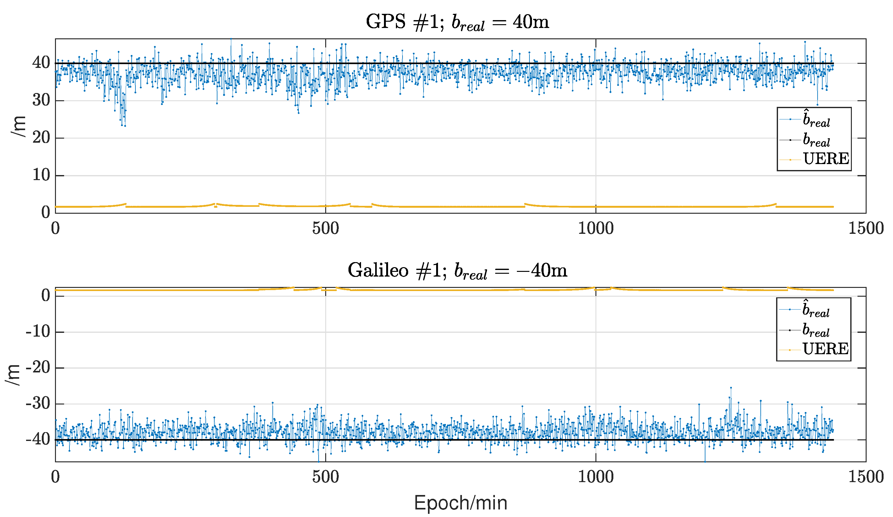
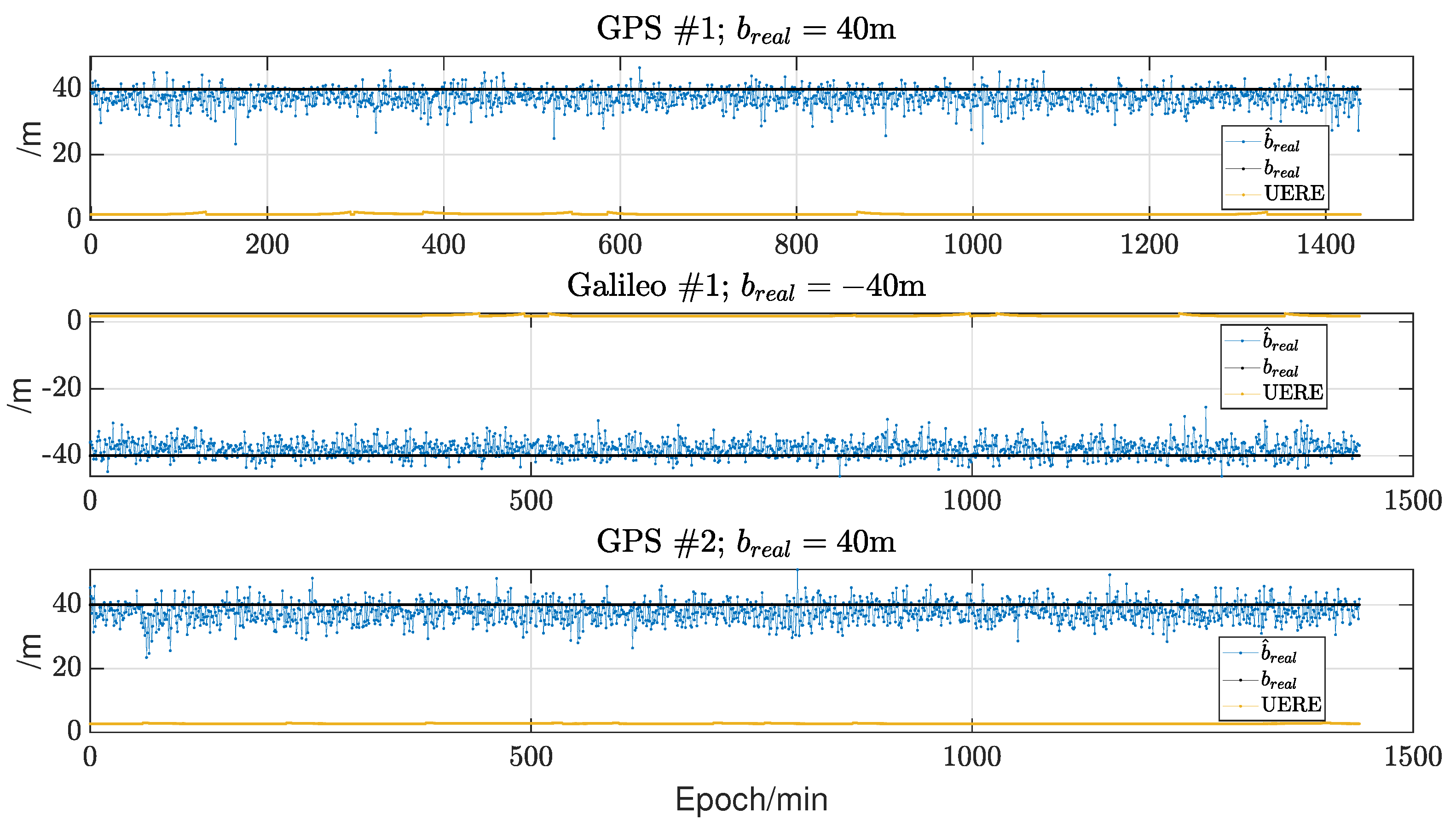
The larger the UERE of a pseudorange, the more the deviation in that pseudorange should favor the nominal error rather than the fault bias . In other words, the higher the UERE for a pseudorange, the closer the estimated value for should be to zero. Therefore, a covariance matrix consisting of the square of the UERE is a suitable weight matrix.
For the specific algorithm design, the crux is to transform the estimation of
into the standard LASSO, according to Equation (
29). According to Equations (
2), (
31), and (
32), we can initially formulate the problem of sparsely estimating
as follows.
Equation (
33) is our core model for estimating
, which is derived via reweighted-
LASSO. In order to make Equation (
33) exclusively comprise the unknown variable
,
is converted into
Equation (
34) can be obtained from Equation (
2) using least squares, which reflects the consistency of the fault-free pseudorange. It can also use weighted least squares. However, to simplify the variable transformation and because the weights already constrain
, additional weighting for Equation (
34) does not significantly improve the results. Therefore, using simple least squares is appropriate.
Substituting Equation (
34) into Equation (
33), we have
After performing variable replacement, Equation (
35) is transformed into
where
and
is the
identity matrix.
Equation (
36) is precisely the standard LASSO problem. At this point, estimating
becomes straightforward. We solve Equation (
36) to obtain solution
and yield the estimated bias vector
:
Equation (
36) has efficient solution methods, such as coordinate descent (CD) [
25] and the least angle regression method [
26]. We choose the classical CD method for solving LASSO, which iteratively progresses along the coordinate axes’ directions until convergence is reached.
Appendix A describes how to solve Equation (
36) and illustrates that its computational load is typically low.
In addition, there is no need for extensive tuning of the regularization parameter
. This is because the primary focus is identifying which elements of the estimated vector
are non-zero rather than precisely quantifying the magnitude of these non-zero values. We have selected the commonly used value of
= 1 for simplicity, and research using sparse estimation for GNSSs suggests that
= 1 is a robust choice that can effectively ensure the estimation accuracy [
14].
As a summary,
Table 1 presents the algorithm for directly estimating faults using reweighted-
LASSO. This algorithm is quite simple: it involves “variable substitution to form a standard LASSO” followed by “solving the LASSO”. The proposed algorithm serves as a solid complement to the existing normalized solution separation statistic method, and both methods can be applied sequentially. Considering the advantages of sparse estimation principles and the experimental results discussed in
Section 5, we recommend initially employing our method for rapid, one-time identification of the exclusion candidates. If this approach fails to identify the candidates, the normalized solution separation statistic method can then be applied. This recommendation is further explained in
Section 6.
6. Conclusions
Finding exclusion candidates is crucial for the swift and successful execution of the ARAIM process. The existing methods infer the likelihood of specific fault modes being actual faults through normalized solution separation statistics, guiding the search for exclusion candidates. However, our qualitative analysis and experimental results indicate that solution separation statistics are not reliable indicators in scenarios involving multiple faults.
This work presents an alternative supplementary method for identifying possible exclusion candidates. Considering the sparsity of GNSS faults and the consistency of normal observations, we propose using sparse estimation to find faulty pseudoranges directly, thus rapidly and efficiently determining the exclusion candidates in a single run without the need for sorting and sequential searching.
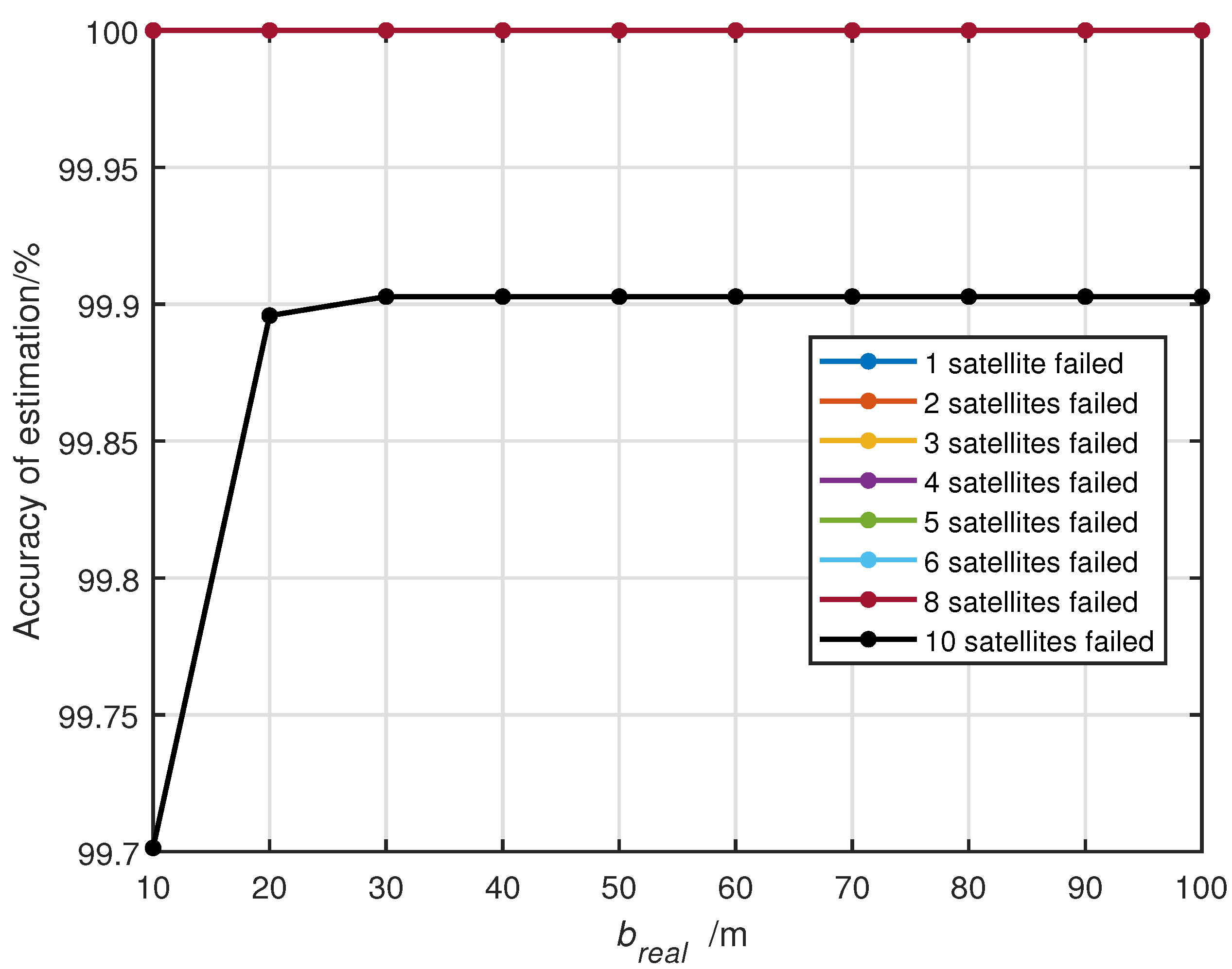
Our experiments demonstrate that the proposed method performs exceptionally well under sparse conditions, being fast and accurate. However, it must be acknowledged that while the sparsity requirements are relatively lenient (e.g., in a dual constellation, it can identify faults among five satellites, and in a quad constellation, it can make estimations for up to ten satellites), this method may struggle with wide faults affecting entire constellations, as such faults are rarely sparse. Therefore, we recommend combining our proposed method with the existing approaches: first, execute our method due to its rapidity. If the exclusion candidates cannot be verified, only the resources for one MHSS test have been expended. Subsequently, the existing approach can be employed, especially focusing on constellation-wide faults. Indeed, the method proposed in this paper is a strong complement to the existing normalized solution separation statistic methods.


