
On a Correlation Model for Laser Scanners: A Large Eddy Simulation Experiment


Institute for Meteorology and Climatology, Leibniz Universität Hanover, 30167 Hanover, Germany
Remote Sens. 2024, 16(19), 3545; https://doi.org/10.3390/rs16193545
Submission received: 20 June 2024
/
Revised: 11 September 2024
/
Accepted: 20 September 2024
/
Published: 24 September 2024
Abstract
:Large Eddy Simulations (LES) allow the generation of spatio-temporal fields of the refractivity index for various meteorological conditions and provide a unique way to simulate turbulence-distorted phase measurements as those from geodetic sensors. This approach enables a statistical quantification of the von Kármán model’s adequacy in describing the phase spectrum and the assessment of the validity of common assumptions such as isotropy or the Taylor frozen hypothesis. This contribution shows that the outer scale length, defined using the Taylor frozen hypothesis as the saturation frequency of the phase spectrum, can be statistically estimated, along with an error fit factor between the model and its estimation. It is found that this parameter strongly varies with height and meteorological conditions (convective or wind-driven boundary layer). The simulations further highlight the linear dependency with the variance of the turbulent phase fluctuations but no dependency on the local outer scale length as defined by Tatarskii. An application of these results within a geodetic context is proposed, where an understanding and solid estimation of the outer scale length is mandatory in avoiding biased decisions during statistical deformation analysis. The LES presented in this contribution support derivations for an improved stochastic model of terrestrial laser scanners.
1. Introduction
Atmospheric turbulence limits the performance of many laser applications by introducing beam wander, beam spreading, loss of spatial coherence, or irradiance fluctuations [1,2,3]. Variations of the detection range, decreased tracking accuracy, or blurring of the image contrasts occur as a consequence. A good understanding of how turbulence affects optical propagation helps reduce these deteriorating effects and offers estimates of the performance degradation that can be imputed to turbulence. In this context, significant turbulent structures generated by buoyancy or shear [4] play a crucial role, being accountable for phase noise at lower frequencies and influencing various optical systems [5,6]. These structures correspond to the end of the Kolmogorov inertial range, i.e., the so-called outer scale length where, most probably, isotropy starts to weaken. plays an important role as the size of telescopes increases [6,7], but also for geodetic sensors for which the stochastic model needs to account for correlations to avoid biased and overoptimistic statistical test decisions in deformation analysis [8]. As is linked with the long-range dependencies of the observations, any improvement in its characterization will be favorable to the setup of a stochastic model without relying on an iterative procedure based, e.g., on residual analysis from surface fitting [8]. This outer scale length, called cutoff frequency in the temporal domain, is the focus of the present contribution.
In this article, is defined as the “scale for determining the transition between inertial and buoyancy ranges” as in [9,10]. This way, Ref. [11] is followed, for whom is “the spatial coherence outer scale of the perturbed wavefront”, in opposition to the local outer scale length as derived from Tatarskii’s definition relative to temperature measurements [7]. has been measured using interferometric or Shack-Hartmann and dedicated instruments such as the Generalized Seeing Monitor and the Monitor of Outer Scale Profile. Table 1 in [6] presents a comparison between various studies highlighting the large range of values depending on the site under consideration (meteorological and topographical conditions), and the measurements (data rate, accuracy). A lack of homogeneity regarding the retrieval of combined with a problem of definition (local or not) may have caused discrepancies. In this context, the present contribution aims (i) to address the challenge of defining and analyzing by comparing it with , and (ii) to derive an approximate atmospheric correlation model for terrestrial laser scanners (horizontal propagation). To achieve this, I propose a statistically-based method to estimate from the spectrum of simulated phase fluctuations using advanced atmospheric simulations with Large Eddy Simulations (LES). To the best of the author’s knowledge, this is the first time such high-fidelity simulations have been employed to model the atmosphere in a geodetic context. LES offer a controlled and reproducible approach to resolving most turbulent motions, enabling the study of the dependence of (and ) on height under various atmospheric conditions. These profiles are crucial for a more comprehensive understanding and quantification of the influence of turbulence on optical wave propagation. They can be used for deriving improved stochastic models that are mandatory in, e.g., statistical deformation testing in geodesy, as proposed in [12], but also for wavefront slope and scintillation correlations recorded with a Shack–Hartmann wavefront sensor [13], or for GEO-feeder link optimization [14] and the references inside. This study has, thus, a wide range of applications.
Phase screens are usually employed for modeling scalar waves in a variety of contexts, such as atmospheric propagation [15]. They can be generated by the subharmonic complemented discrete Fourier transformation, randomized spectral sampling techniques, and optimization-based method [16]. The Zernike series method is widely used; It allows determining the outer scale length and the structure constant based upon sequential analysis of normalized correlation functions of Zernike coefficients [15,17,18]. Because measured fields of the refractive index are often not available along the whole propagation path, the phase screening approach often uses the assumption that the refractivity index spectrum should follow a given model [17]. The von Kármán spectrum and its variations are popular choices but the Hill spectrum can also be used, see [19] for a comparison of the spectra. In this contribution, a methodology as proposed [20] for electromagnetic wave propagation is followed: LES output (gridded temperature, pressure) will be used to relax the assumption about the refractivity index spectrum and generate temporal phase measurements from the LES-simulated 4D refractivity index field itself. Thus, virtual (plane) waves are simulated corresponding to propagation in a simulated yet highly realistic atmosphere. The advantage of this method is to manage and manipulate the experiment effectively. I refer, e.g., to [2,3] who investigate the effects of intermittency on laser propagation. In this contribution, the Rytov approximation is assumed for a plane wave corresponding to a LiDar sensor as, e.g., a laser scanner with a wavelength around 900 nm. I focus on horizontal propagation in this contribution regarding the targeted applications (terrestrial laser scanner) and reduce the general wave propagation equation to a first-order parabolic equation [1,21]. The turbulent parameters and the phase variance are estimated using an improved and dedicated statistical method called the debiased Whittle Maximum Likelihood Estimation (WMLE) [22], which was adapted to the context of estimating the outer scale length. Other methods are based on, e.g., upon sequential analysis of normalized correlation functions of Zernike coefficients as proposed in [23]. The main advantage of the WMLE is that it does not rely on visual inspection or regression on the spectrum as in [24] or some comparison with typical spectra [11]. It is assumed only that the spectrum should follow a Matérn model with a given power law (e.g., the Kolmogorov one) to estimate statistically the parameters and their uncertainty [25]. Whether this model is accurate is still an open question and beyond the scope of this contribution: Its main advantage is to avoid an infinite growth of the variance at low frequencies. Through this contribution, the Taylor frozen hypothesis is supposed to be valid to switch from a spatial to a temporal representation [26]. A significant degree of error fit between the true (or assumed) model and the estimate can be associated with deviations from this assumption, in the case of anisotropy [27] or non-Gaussianity. The proposed statistical method allows such investigations.
To investigate various turbulent conditions encountered in real propagation cases, three different turbulent regimes are simulated: buoyancy or shear dominantly, and a combination of both. These setups mimic different solar and thermal forcings or geostropic wind. The dependency of and with height is investigated, and how is empirically related to the strength of turbulence in the inertial range following the goal to derive a simple correlation model. Through a nesting procedure in LES, the estimation of these quantities near the ground is made possible.
This study is based on simulations and:
- estimates from simulated phase spectra for various meteorological conditions with a statistically based method rather than an empirical one,
- provides new insights into and its variability with height depending on the turbulent conditions (wind shear, buoyancy) to derive an atmospheric correlation model for terrestrial laser scanners,
- allows gaining a better understanding of its relationship to the local as derived by Tatarskii and measured by radiosondes to avoid confusion.
The remainder of this contribution is as follows: in Section 2, the principles used to generate phase measurements and how the parameters of the von Kármán spectrum can be statistically estimated are introduced. I further discuss the LES setup and the various atmospheres simulated in the Section 2.6. Section 3 and Section 4 are dedicated to the presentation and discussion of the results.
2. Methods: Wave Propagation and Large Eddy Simulation
The first part of this section introduces the propagation through a simulated atmosphere and derives the spectrum of phase measurements. The estimation of the spectrum parameters (outer scale length, variance, slope) with the WMLE is developed and the LES setup to simulate realistic atmospheres in which the signals can propagate, described.
2.1. Wave Propagation through Simulated Atmosphere
Atmospheric turbulence generates refractivity index fluctuations which in turn causes amplitude and phase fluctuations of propagating electromagnetic waves. In this contribution, I restrict myself to plane waves from a scanner (wavelength approximately 900 nm, high coherence length for long propagation distance [28]) as an example and without lack of generality regarding other sensors. The impact of humidity is further neglected [29,30]. The far-field condition is met for the setups as distances of propagation greater than 40 m for a target having a radius of 1cm are considered. The extension to spherical waves is straightforward and the reader should refer to Chapter 17 in [21].
The principle of the three-step methodology is summarized in a flowchart form in Figure 1:
- Simulation of a spatio-temporal 4D field of temperature and pressure using LES as described in Section 2.6.
- Generation of phases starting from the Rytov approximation. More specifically, I make use of the Rytov first iteration solution for the phase. This latter is known to be valid also in the strong fluctuation regions [31]. Its exponential representation is favorable to represent a wave propagating through a random medium.
- Statistical estimation of the parameters of the power spectrum from the generated phases propagating in the simulated atmosphere (from the first step). I fully exploit the potential of LES to determine the temporal refractivity index fluctuations at any location along the propagation path using virtual measurements [32]. Thus, I do not rely on any apriori model as in [33], and the references inside.
The derivation for the phase expression starts with the Maxwell’s equation for a fluctuating medium:
corresponds to twice the refractivity index fluctuations for a weakly turbulent medium and we skip the temporal dependencies in the following derivations for the sake of readability. is the y-component of the electric field assuming a wave propagation in the direction of the x-axis. k is the wavenumber. The wavelength in the optical region is considered to be much smaller than the scale size (correlation length of the refractive index fluctuation) of the random medium. is expanded in a series and express as a solution of the first order Riccati equation: . A plane wave propagation over a distance (distance target/receiver) is considered, as graphically explained in Figure 1b with the example of a geodetic laser tracker. Under these assumptions, is expressed as
is decomposed into with representing the log-amplitude fluctuations and the phase fluctuations. An expression for the phase follows:
with being the imaginary part of
Equation (3) simplifies for the chosen setup to . This derivation assumes that the major contribution to comes from the region and which is justifiable if one considers a small pipe along the propagation line of sight as the integration region. Homogeneity of the medium along the propagation path is here mandatory and given from the LES setup. It can be relaxed by dividing the integral into homogeneous domains for real cases (with heterogeneous surfaces).
2.2. Refractivity Index
The phase at is a time-dependent variable through . Following [21] or [34], the refractivity index n is expressed as . is a function that depends on the optical wavelength and is often approximated to . An adiabatic process with no loss or gain of heat to a volume of air is assumed. Under these assumptions, the refractivity index fluctuations simplify to with . is the ratio of the specific heat at constant pressure to constant pressure for the atmosphere. These quantities can be estimated from the LES at each time step and grid point. corresponds to variations of around the temporal mean at a given location.
The integral in Equation (3) is replaced by a sum and I perform the numerical integration using the trapezoidal rule [35]. To that aim, the horizontal path at each height step is divided into regular segments. Above 100 m, 50 segments of 20 m and a height step of 50 m are chosen to save computational time. Below 100 m, a height step of 2 m using nesting in LES is considered, i.e., a “zoom” in the main domain. is computed from the LES at those specific grid points as illustrated in Figure 1a where 5 points are depicted to ease visualization. The value of at one point is considered to be valid in the entire integration volume , as for the phase screening method. The elongation of along the y- and z-axis should be much smaller than along the x-axis. I have chosen and tested that small variations around this value did not affect the results significantly (variations within the 1 rule).
Under these assumptions, we get a temporal expression for the phase at the target after horizontal propagation at a given height expressed as . The power spectrum of the phase is expressed as:
where is the average operator. The horizontal propagation was chosen to derive height profiles of the quantity of interest following the investigations in, e.g., [29]. An oblique path can be easily considered thanks to virtual measurements in LES.
2.3. Theoretical Power Spectrum of Phase Fluctuations
The statistical properties of turbulence can be expressed with the spatial structure function of any passive tracer , as the potential temperature or the index of refractivity n as follows
where x is a position vector, r a spatial displacement. Using the Kolmogorov assumption for isotropic turbulence, I have , which is valid in the inertial subrange. is called the structure constant for the scalar . Tatarskii [36] showed that this parameter can be related to a scale of turbulence called here as follows with the gradient of the mean of . [37] proposed a formulation for the local which reads:
with g the gravity acceleration, the turbulent kinetic energy, a quantitative measure of the intensity of turbulence for a given flow, and the virtual potential temperature. does not correspond to : These are two parameters with different derivations. An improved formulation of Tatarskii’s scale lengths was proposed in [10], depending solely on certain variances and mean gradients. For simplicity, the most common option was chosen, as the focus of this contribution is on the outer scale length of turbulence , rather than the local scale [7].
From the preceding equations, it is possible to derive a spatial structure function for the phase, as outlined in Chapter 5 of [38], which details the statistical properties of phase differences measured between spaced receivers [39]. In this contribution, the statistical properties of the temporal phase variations at the target are the main focus, a quantity that can be measured, see Equation (3). Therefore, the same approach employed for the spatial case can be utilized to formulate a temporal phase structure function, i.e., , with a time increment [38] (Chapter 6.2.2).
The phase spectrum is preferably used for real case applications. It is linked to the temporal covariance by the Wiener-Khinchine theorem as in Equation (5). Assuming isotropy of the medium and wind blowing horizontally at a constant speed with a direction orthogonal to the propagation, it can be shown that where is the Bessel function of 0th order and the geostropic horizontal wind speed. Using the von Kármán model of turbulence and the Taylor frozen hypothesis [26], an expression of the phase covariance can be derived, followed by the theoretical phase power spectrum. To that aim, a simple coordinate translation is performed to replace the distance scaled by the velocity of the irregularities by the time, i.e., phase covariance between adjacent time is considered to be identical to the spatial correlation between parallel rays separated by a vector . This approximation involves two assumptions: (i) the medium is frozen during the measurement interval, which is justifiable due to the high scanning rate of most devices (below 1 s) and (ii) the variable component of the wind velocity is neglected. In the case of spatial measurements, this corresponds to a constant velocity along the path at each location. This assumption leads to an expression for the temporal phase spectrum as derived in Chapter 6 of [38]:
with . A discussion on the validity of this assumption is provided in [40]. Here, I follow [9,41,42] and define as “the scale for determining the transition region between the inertial and buoyancy ranges”, which corresponds to the saturation or cutoff frequency of the temporal power spectrum, with . This scale was related to the Brunt-Vaisala frequency of the atmosphere at the height of the measurement and the rate of dissipation of the turbulent kinetic energy . For shear-driven turbulence, Ref. [9] shows that . This formula is case-related and its validity is not investigated in this contribution. However, it lets us think, intuitively, that could be linked with the variance of the phase turbulent fluctuations defined below.
Equation (8) corresponds to a Matérn spectrum in statistics [25] which can be written in a simplified form as
with . This spectrum is described by three parameters: the variance , the slope , and the transition or cutoff frequency . Here the growth induced by turbulence is symbolized by the forcing parameter, which corresponds to the slope of the power spectrum density (psd) denoted as . From physical considerations, some resistance should be put on that growth, which is modeled by the damping parameter . According to the Kolmogorov theory, the slope is predetermined to , leaving two parameters to estimate which are the transition frequency (associated with the outer scale length of turbulence and the mean wind ), and the variance of the turbulent phase fluctuations . The reader should refer, e.g., to [43] for a discussion on the Kolmogorov assumption.
Using Equation (8), the relationship
can be derived. This expression allows computing the popular using a mean value of the wind velocity from the LES at a given height and the estimated . This topic falls outside the scope of the current study.
2.4. Whittle Maximum Likelihood Estimation (WMLE)
The Debiased WMLE
The estimation of turbulence parameters [, , ] from the empirical temporal spectrum of observations relies often on iterative regressions as described in [24], or on the covariance function, either spatial or temporal [11]. In this contribution, I propose an alternative method based on the theoretical knowledge that the spectrum follows the one of a Matérn process as described in Equation (9) [25,44]. The transition frequency as well as the variance and the slope can be estimated using a debiased version of the WMLE [22]. This procedure has been demonstrated to be suitable for small sample sizes which is particularly advantageous given that the stationarity of phase fluctuations is only valid for 30 min (1800 samples at a data rate of 1 s).
Exact maximum likelihood inference can be performed for Gaussian data [45] by evaluating the log-likelihood , means the covariance matrix of the observations and the residuals vector after the least-squares approximation. Matrix inversions can be avoided using the Whittle estimator, which aims to provide faster estimation with only a slight inaccuracy. In that case, the log-likelihood is simply approximated in the frequency domain. Unfortunately, the formulation is based on the periodogram which is known to be a biased measure of the continuous-time process’s spectral density for finite samples and real data due to additional blurring and aliasing effects. To face that challenge the debiased Whittle likelihood was introduced, and is given in its discretized form by , with the set of discrete Fourier frequencies, the expected periodogram, given by the convolution of the true modelled spectrum with the Fejér kernel and is the periodogram with . E is the expectation operator. A white noise component can be estimated conjointly, which may be interesting for real data applications in the presence of additional sensor noise [11,46].
Please further refer to [22] for more details on tapered WMLE to reduce data blurring. This method consists of pre-multiplying the data sequence with a weighting function known as a data taper. I have chosen the widely used Slepian taper in this contribution following the proposal of [25].
The main limitation of this method is the Gaussian assumption of the phase measurements, potentially untrustworthy as shown in [29]. I prevent myself from such a deviation by (i) using simulated time series that are long enough, and (ii) computing a statistical model error. This global measure called in the following, is the degree of error fit between the natural log of the periodogram and that of the fitted spectrum. It can be estimated by computing the mean squared error between the two quantities. The helps detect challenging cases where the Kolmogorov assumption may fail due, e.g., to anisotropy [47]. The debiased WMLE is less sensitive to deviations from normality compared to the maximum likelihood estimator, and it should enable the estimation of the outer scale length even under conditions of significant fluctuations.
In this contribution, is estimated from the cutoff frequency and the variance of the process by fixing the slope to during the estimation process. The slope may not follow exactly the Kolmogorov assumption for some cases or due to numerical dissipation in LES. To face that challenge, the slope is allowed to be fixed as a constraint within a given interval (+/−10% of ) during the estimation. To avoid several minima in the WMLE, is also restricted from physical considerations knowing that should be between 50 and 6000 m following [38] for a geostropic wind velocity between 1–10 ms−1. This corresponds to the ranges of values chosen for our LES setups (Section 2.6, Table 1).
I emphasize that an increase of indicates that either (i) the von Kármán spectrum may not be the best one to describe the turbulence fluctuations of the refractivity index, (ii) the Gaussian assumption may be strongly violated, or (iii) the Taylor frozen hypothesis is inadequate [48]. Numerical dissipation may also come into play, although this risk is strongly limited by our LES setup Section 2.6. Thus, the length of the simulated time series should be long enough to allow for the saturation of the psd in the low-frequency region, whose occurrence depends on the LES input parameters (shear-driven or convective turbulence). The length in the LES is fixed to at least 6000 samples to allow for saturation. If this one does not occur, will strongly increase as a diagnostic. The variance defined as the variance of the underlying Mátern process is linked but not directly proportional to the structure constant of the refractivity index as specified in Equation (10).
2.5. LES: Principle
The present investigations are based on simulated turbulent atmospheres, for which input parameters such as the geostropic wind velocity or the surface heat flux can be controlled. This enables the simulation of dynamics in boundary layers driven by shear, moderate convection, or free convection. In this contribution, the PArallelized Large Eddy Simulation model (PALM [49]) is used. The model solves the governing prognostic equations on a Cartesian grid using finite differences. Spatial discretization is performed by the default fifth-order advection scheme [50]. The spatially filtered Navier-Stokes equations governing the atmosphere can be solved down to scales in the inertial-convective range. The flow is treated as incompressible but allows for variations in density due to buoyancy. Consecutively, the pressure P is approximated as , where are the LES pressure fluctuations. The temporal discretization is achieved by a third-order Runge–Kutta time-stepping scheme as described in [39]. An additional prognostic equation for the subgrid-scale turbulence kinetic energy uses the 1.5-order subgrid closure after [51].
For the whole area, cyclic boundary conditions were chosen at all edges. A constant flow layer was assumed as a boundary condition after Monin-Obukhov similarity theory between the surface and the first lattice level [4]. Further boundary conditions were set as far as necessary and included following the default selection of the model. The boundary layer was topped with an inversion with a potential temperature gradient of 1 K per 100 m above 800 m. To avoid strong variations of the boundary layer height constant for the duration of the simulation, a large-scale subsidence of −0.015 ms−1 was applied at 1000 m and above, which decreased linearly to zero between 1000 and 0 m. Scalar quantities such as temperature or pressure are defined at the center of the grid volumes and are not further interpolated. For this study, PALM in version 22.10 is used, and the facility of the Norddeutsche Verbund für Hoch- und Höchstleistungsrechnen (HRLN).
2.6. LES: Simulation Setup
Horizontal wave propagation along the x-axis is simulated, as described in Section 2.1. The distance between the virtual target and the receiver, such as a laser scanner, is set to 1000 m. The virtual measurement module of PALM is used to extract the temperature, pressure, and wind velocity at 51 points (50 segments) separated by 20 m along the virtual path. I recall that the temporal phase fluctuations at the target after propagation through the random medium (no double-path propagation) are of interest in this contribution.
Three cases corresponding to various geostropic forcing and surface heating were chosen to generate different types of flow regimes, from buoyancy-driven (case 2) to shear-driven (case 3) flows. A moderately convective situation with a geostropic wind of 5 ms−1 and surface heat flux of 0.05 Kms−1 is chosen as an intermediate case (case 1). Further, the geostropic wind was set to blow along the y-axis so that 0 ms−1. Following [41], should vary depending on the buoyancy characteristic of the boundary layer as shown in real cases with generalized seeing monitor [11]. Table 1 summarizes the LES setups.
For all simulations, a domain size of 10 × 10 × 3 km3 was chosen following [52] and [29] and a size of 1 × 1 × 0.2 km3 for the nested domain. The development of large turbulent structures is given through a sufficiently large horizontal extension of the parent domain, which is used to initialize the nested domain [53]. All simulations are carried out over a homogeneous and flat surface with a roughness length of 0.05 m (grass). I start the virtual measurements at a height of 100 m every 50 m and in the nested domain at a height of 0.5 m every 2 m.
Comment on the grid spacing A grid spacing of 5 m was chosen, respectively 2 m in the nested domain. Regarding the high coherence length of a geodetic laser scanner -necessary to ensure a long propagation through the atmosphere-, I consider the grid spacing as appropriate. To account for numerical dissipation, the effective grid spacing is considered to be 5 times higher (worth case) than the real grid spacing which corresponds to 25 m in our case (10 m in the nested domain, respectively). The internal time step from PALM with this configuration was 0.1 s (0.05 s in the nested domain). Assuming the Taylor frozen hypothesis to hold (which is highly plausible at that rate), this corresponds to a minimum or effective frequency that can be resolved in PALM of 10/5 = 2 Hz; Thus, for a low wind velocity of 1 ms−1 (convective case as described in Table 1), can go down to 1/2 = 0.5 m with the proposed configuration. Decreasing the grid size is associated with a high computational burden and energy resources. The smallest (and somehow controversial) values found in the literature [7] are around the chosen grid size, and more realistic values are around the effective grid size of the non-nested domain. I further conducted a simulation run for a selected case, reducing the grid size to 0.5 m. This adjustment (not presented for the sake of conciseness) did not affect the results nor the conclusions of this study.
Boundary conditions are set to be cyclic in all lateral directions. To prevent gravity waves from being reflected at the top boundary, a Rayleigh damping is applied to all prognostic variables from 1450 m [54], i.e., within the free atmosphere.
The onset of turbulence is triggered by random perturbations with small amplitudes imposed onto the horizontal wind field during the initial stage. A spin-up period of 5000 s was chosen after which quasi-stationary is reached. The simulations started from that point and lasted 6000 s in total to ensure the aforementioned saturation of the psd at low frequencies. The time step from PALM was averaged for each setup but did not vary significantly around the mean to affect the estimated parameters. I have output the LES values every 0.1 s resulting in a sample frequency of 10 Hz. I acknowledge that geodetic laser scanners have a much higher scanning frequency. However, increasing the scanning frequency necessitates decreasing the grid size and will mainly introduce power at high frequency (white noise), thus not affecting the low-frequency region of the spectrum.
For each of the three cases, 10 simulations were carried out by changing the random initial conditions to save computational resources. The values were averaged and their standard deviation was computed [32]. For the nested cases, only one simulation was carried out to save computational time and resources but a spatial average was performed within the simulated atmosphere, i.e., 10 paths were considered and averaged.
3. Results
3.1. Presentation of the Results
To investigate the extent to which and vary with the simulated turbulent conditions, the methodology presented in Section 2 is followed. More specifically I:
- generate three turbulent atmospheres following Table 1 using LES as described in Section 2.6,
- simulate an optical wave propagating along the x-axis, perpendicular to the geostropic wind component [38] and set m,
- estimate statistically the cutoff frequency , the parameter and the variance using the debiased WMLE,
- compute for the inertial subrange following Equation (7). I compare this value to the one found in step 3.
The steps from 2–4 are repeated by varying the height of the horizontal path to generate height profiles. The objective is to measure the degree to which the values change with height along an oblique trajectory through a turbulent atmosphere. The LES profiles are averaged when the boundary layer has reached a quasi-steady state. Here I investigate spatially average profiles of , the wind velocity v (norm of the wind vector), the total vertical turbulent sensible heat flux , (the sum of the variance of the resolved u- and v-velocity components), and , the variance of the vertical w-velocity component. Ref. [55] is followed to define the anisotropy ratio as . For isotropic turbulence, whereas for weakly stable regime, 5–8 [56].
The investigations are empirical and do not aim to derive a general formulation at that point; This latter may not cover all possible cases of turbulent conditions.
For each case under consideration, the average profiles are described before commenting on , , , and the ratio . This latter indicates if the variance of the turbulent phase fluctuations is related to the outer scale length by a simple mathematical relationship, which would grandly simplify the setup of an improved correlation model for terrestrial laser scanners. All first subsections are devoted to the height profiles starting from 100 m. In the last subsection, the nesting cases are investigated separately.
3.2. Case 1: Mixed Turbulence
We start the investigations with case 1 of Table 1, which corresponds to a mixed shear- and buoyancy-driven turbulence.
Average profiles
The validity of the LES is checked using the average profiles. The wind velocity v reaches the expected value of 5 ms−1 at the first LES grid point (Figure 2b). starts increasing with height from the boundary layer height (800 m), as expected from the LES setup (Figure 2a left). (Figure 2a middle) decreases with height until the boundary layer height. The variance of the horizontal velocity component (Figure 2a right) decreases with height until it reaches a minimum value at 400 m and a maximum at 800 m. (Figure 2b left) reaches a maximum at 300–350 m (first inflection point of the curve), slightly lower. increases from the height of 400 m to 800 m similarly, which is a coherent shape compared to the other profiles.
α and
The cutoff as presented in Figure 3b can be thought of as a temporal “outer scale”, i.e., non-scaled by the horizontal wind velocity. It decreases with height up to the boundary layer height but does not present an inflection point at a lower height (refer to the average profiles such as the vertical velocity component as an example). The profile of (red line in Figure 3a) follows the one of the horizontal wind velocity. can be considered as nearly constant with height, having only a weak infection point around 300 m. follows the profile of well from 100 m up to 800 m and could also be used as an alternative to quantifying anisotropy. Further, strongly increases from 700 m, as increases. Conversely, the profile of with height exhibits similarities with that of the variance of the vertical wind velocity, a relationship strongly supported by Equation (7) [7]. The mean value is slightly higher than and around 30 m but no linear relationship between the two quantities can be deduced as in [57], which is most probably due to the different strategies used to compute the quantities (statistical/empirical). As aforementioned, is nearly constant with height. The range of values found validates the chosen grid spacing.
The sampling frequency is Hz, resulting in a mean value of of 25 m between 100 and 800 m height. The values from 850 m (as the LES results in general above the boundary layer height) are less trustworthy but show a strong increase of , which stays, however, plausible as the horizontal elongation of the eddies may be more pronounced. From this comparison, could be linked with the size of turbulent structure for mixed turbulence, see [38].
The ratio R of is constant with height (Figure 3c), highlighting that a direct scaling could be deduced from the outer scale length and the strength of turbulence in that case.
Figure 3d highlights that the error between the model and the simulated observations increases linearly with height, which could be related to a deviation from the Gaussian assumption as stated in [52]. For a deeper investigation, the probability density function of are plotted in Figure 4a. Here the increase of kurtosis with height is evident up to 600 m. The high kurtosis is probably due to strong low-frequency fluctuations and not to outliers as shown in Figure 4a,b. A log-normal probability distribution is more adequate to describe the simulated observations as confirmed in real case [7].
Thus, I would tend to interpret the as a difficulty in simulating optimally the turbulence in LES as the height increases. The spread of value of both and is small, which highlights the high trustworthiness of the height profile, considering that only ten LES were averaged.
3.3. Case 2: Convective-Driven Turbulence
The LES simulations were repeated for case 2, which corresponds to convective-driven turbulence (free convection) as in [52].
Figure 5 highlights that the boundary layer height is slightly higher than for case 1 (850 m compared to 800 m). Here the strong buoyancy due to the low wind shear is associated with well-developed convective structures, responsible for a higher boundary layer. This effect is damped by our LES setups as described in Section 2.6. The variance of the horizontal wind component is low, decreases linearly with height, and has no inflection point. On the contrary, the vertical wind component reaches a maximum at 350 m, similar to the profile of in Figure 3b (red line with circles). is lower than for case 1 (in mean 15 m) and gets smaller as the height increases. Thus, the convective plumes are admittedly larger but their size decreases with height up to the boundary layer height (850 m). At the same time, (Figure 3d) is constant with height but higher than for case 1 which could be linked with non-Gaussianity, or a challenging estimation due to a non-Kolmogorov turbulence or non-validity of the Taylor frozen hypothesis. The violation of the homogeneity assumption, i.e., when no mean background wind is present is plausible as turbulent structures should be stationary during their life cycle [32]. I intend to think that the turbulent structures are becoming increasingly anisotropic in the inversion layer, which is also linked with an increase of . I note that the transition region between 700 and 900 m, i.e., before increases, is much wider than for case 1, which I attribute to the smoother shape or shallow curvature of (Figure 5b). I repeated the statistical investigations on as in Figure 4 and found similar dependencies. The corresponding figures are not shown for the sake of conciseness.
From Figure 3c, the ratio R is not constant with height and shows an inflection at 700 m, a point where the variance of the horizontal wind component starts to increase slightly (Figure 5a right). A light linear relationship exists below that height highlighting the dependency of the two parameters for given simulated conditions. Unfortunately, no plausible explanation for this finding can be given at that stage. The value of is here difficult to interpret due to the small temperature gradient with height [9].
3.4. Case 3: Shear-Driven Turbulence
Average profiles and outer scale length
Figure 6 shows the average profiles from the LES for case 3, which corresponds to shear-driven turbulence with 10 ms−1 and Kms−1. The variance of the vertical wind velocity has a similar shape compared to cases 1 and 2. The first inflection point is reached at a height of 350 m, slightly higher than in case 2 (convective-driven) and at the same height as . The anisotropy is much stronger (by a factor 2) at the boundary height than for cases 1 and 2. From Figure 3b (dotted red line) I see that increases linearly with height up to 350 m, and stays constant from 400 m up to the boundary layer height. has a mirrored profile, slightly decreasing and increasing again correspondingly. The profile is similar to case 1 although the two conditions are different due to the scaling with the horizontal wind velocity. The small makes us confident about the trustworthiness of the comparison with case 1 (Figure 3d). On average, the value of is slightly higher (30 m), a difference which I won’t overinterpret. varies stronger with height, with a maximum close to 50 m as the vertical wind velocity, thus confirming the adequation between the two parameters and the fundamental differences between and .
The anisotropy increases from 600 m, where the shape of starts having similarities with the one of case 1, which would link with more elongated structures present in both cases at that height. The ratio R has a linear dependency (positive slope) up to that height and shows a negative slope after 600 m, i.e., no direct scaling but a dependency with anisotropy. The smaller value of for case 2 decreases the impact of buoyancy in the lower boundary layer to the benefit of a “shear-driven like” turbulence profile up to 200 m as seen in Figure 3c. The power spectral density (not shown) followed the Mátern spectrum with high confidence, even above the boundary layer height.
Nesting: m
Many optical devices such as geodetic laser scanners operate near the ground both indoors or outdoors, see [58,59,60] as examples. To investigate the variability of at that height more accurately, I perform a nesting (“zoom”) in the main domain as described in Section 2.6. The corresponding results are presented in Figure 7 for the three simulated turbulent atmospheres.
From Figure 7, following conclusions can be drawn:
- similar to the non-nested cases, the variability of of with height is low, particularly for case 2 (convective-driven turbulence). The values found are compatible for all cases with the previous results from m.
- No clear linear dependency neither of nor of with height can be deduced from the analysis but I note that increases linearly with height in the first 10 m above the ground. The slope is the same for cases 2 and 3 and slightly lower for case 1. It cannot be linked to the power laws sometimes found in the literature. increases slightly with height (not shown as similar to the non-nested case) but is higher for the convective case, as in the non-nested simulations. This shape could be related to variations on smaller scales and the stronger impact of the surface layer, i.e., the shorter reorganization rate of the turbulent structure, in that case [52].
4. Discussion and Application
4.1. General Consideration
From the LES results, the convective case shows a different behavior compared to the shear-driven and mixed cases. The value of is 3 times lower (30 versus 10 m) in that case, and linked with a higher . This finding is potentially due to the model assumptions being less valid (gaussianity, Kolmogorov slope, Taylor frozen hypothesis, stronger numerical dissipation in LES). This is reinforced as the shape of the profiles is linked with the one of anisotropy making the Kolmogorov scaling doubtful [43]. The investigation of the reason behind this discrepancy would necessitate additional mathematical tools such as the multifractal spectrum and should be the topic of the next contribution.
The cutoff frequency shows more variability with height compared to as it is not scaled by the wind velocity. Thus, studying sheds light on specific turbulent patterns and atmospheric conditions such as, e.g., the length of the “temporal” inertial range. Further, I found a clear linear dependency with , particularly near the ground in the nested domain, with a slope depending on the simulated atmospheres.
From the analysis of the previous results for the three cases under consideration, it is highly plausible to consider as a constant near the ground (in the first 50 m above the ground), but depending on the meteorological conditions: 15 m for convective conditions (sunny day with low wind velocity with high correlation length) and 30 m for other cases. This finding should allow fixing the parameter as in Equation (9) as a constant depending on the meteorological conditions near the ground. The time of the day (day-night), as well as the surface roughness (e.g., asphalt/grass), or the wind direction, may also play a role although strong deviations from our results are not expected [61]. This is an important finding as it will grandly simplify the setup of a correct stochastic model for geodetic application in deformation analysis [62] or for selecting the best time of the day for measurements.
4.2. Atmospheric Correlation Model
It is known that atmospheric turbulence generates fluctuations that may affect the detection of deformation by correlating the phase measurements [12,63]. A stochastic description of the measurements should include a description of the correlations due to turbulence (variance and outer scale length/cutoff frequency). This study demonstrates that, with a general understanding of atmospheric conditions (such as wind velocity, buoyancy, or shear-driven scenarios), an empirical derivation of the stochastic model is achievable without the need for additional complex meteorological sensors. A computational demanding iterative estimation of the stochastic parameters from residuals (surface fitting) [62] is not mandatory at first to set up the variance-covariance matrices of the measurements [64]. This way, it is possible to improve the uncertainty description of laser scanners to account for correlations. This is indispensable to prevent biased test statistics in highly accurate deformation analysis, such as in bridge or tunnel monitoring and landslide applications [65,66]. For a higher accuracy, the profiles generated in this contribution can be used to setup the atmospheric correlation model and used for oblique paths. I strongly recommend not to deduce the parameter from the local outer scale length from radiosondes, as it does not rely on the same assumptions. This would affect the assumed correlation length accordingly (too high correlation length, underoptimistic test statistics).
5. Conclusions
In numerous applications, including deformation analysis in geodesy and adaptive optics, it is imperative to mitigate the effects of atmospheric turbulence on phase (wave-front) measurements to prevent detrimental impacts. A finite outer scale length (cutoff in the temporal domain respectively) contributes to the long-term dependency of phase measurements, significantly influencing the outcomes of statistical tests [12], and thus, necessitates consideration. The outer scale length is also important within the context of very large telescopes and long-baseline interferometry [6]. To enhance the understanding of this turbulent parameter and its dependency on height and meteorological conditions, LES were used to simulate a full turbulent atmosphere as in real conditions and generate phase fluctuations using the Rytov approximation by varying the surface heat flux and the wind velocity, assuming a wind blowing perpendicular to the wave propagation. A statistically-based method was developed to estimate, from the turbulence theory and with high trustworthiness the frequency from which the Kolmogorov scaling significantly changes (either saturation or slow transition). The Taylor frozen hypothesis was used, which is a plausible approximation in geodesy due to the high data rate of most sensors. We could show that discrepancy from this assumption due, e.g., to anisotropy, manifested itself as a strong misfit between the theoretical spectrum and the measured one which can be statistically assessed with the proposed methodology. The main output of this contribution was to systematically investigate which was found to depend on the LES setups, and, thus, on the meteorological conditions in a real case. Except for convective-driven turbulence for which a value smaller than 30 m was found, reaches 30–50 m (data rate output of 0.1 s). The profiles were nearly constant with height with a departure of a maximum of a few 10 m from the mean so that the cutoff frequency can be easily derived knowing only the horizontal wind velocity at the height under consideration, mostly near the ground. A direct relationship with the local outer scale length from [37] could not be derived. However, a linear dependency of the variance of the turbulence fluctuations versus was found, the slope being case-dependent but similar for shear- and convective-driven turbulence. More simulations are needed to investigate the influence of surface heterogeneities and various roughness [61]. Also, daily variations need to be specifically investigated for permanent laser scanning applications [67]. However, the potential of LES to derive a trustworthy atmospheric correlation model for terrestrial laser scanners from wave propagation in turbulent media was shown, based on simplified yet highly realistic atmospheric conditions. This paves the way for even more realistic simulations, although the proposed simplification based on approximate values of should be sufficient for most applications. This work has demonstrated that an unconventional yet noteworthy use of terrestrial laser scanners could be in assessing turbulence parameters, akin to scintillometers [58], by applying the methodology developed in this study to derive height profiles. An initial attempt in that direction is presented in [68]. Consequently, laser scanners could be used to investigate atmospheric turbulence in the boundary layer (refractivity index fluctuations integrated along the path). Potential applications may be associated with climatological studies, particularly in Alpine terrains where permanent laser scanners are in continuous operation [69,70].
Funding
This study is supported by the Deutsche Forschungsgemeinschaft under the project KE2453/2-1 for correlation analysis within the context of optimal fitting of point clouds recorded by terrestrial laser scanners.
Data Availability Statement
The PALM model system is freely available from http://palm-model.org and distributed under the GNU General Public License v3 (http://www.gnu.org/copyleft/gpl.html). The model source code of version 22.10 described in this article, is also available via https://doi.org/10.25835/0041607. For code management, versioning, and revision control, the PALM group runs an Apache Subversion (http://subversion.apache.org (svn) server). The PALM model system can be downloaded via the svn server, which is also integrated in a web-based project management and bug-tracking system using the software Trac (http://trac.edgewall.org). All time series used in this article are accessible through an open repository hosted at Leibniz University Hannover [71]. All simulation results can be reproduced exactly in Matlab, and the software is freely available at https://github.com/AdamSykulski/SPG.
Acknowledgments
G.K. gratefully thanks the Norddeutsche Verbund für Hoch- und Höchstleistungsrechnen (HRLN) on which all LES computations with PALM were performed. Matthias Sühring is warmly thanked for fruitful discussions, and Pierre Monteyne is acknowledged for his assistance in configuring the simulations.
Conflicts of Interest
The author declares no conflicts of interest.
Abbreviations
The following abbreviations are used in this manuscript:
| LES | Large Eddy Simulation |
| WMLE | Whittle Maximum Likelihood Estimation |
| MDPI | Multidisciplinary Digital Publishing Institute |
| DOAJ | Directory of open access journals |
| TLA | Three letter acronym |
| LD | Linear dichroism |
References
- Andrews, L.C.; Phillips, R.L. Laser Beam Propagation through Random Media; SPIE Optical Engineering Press: San Francisco, CA, USA, 2005. [Google Scholar] [CrossRef]
- Rod, F. Effects of refractive turbulence on coherent laser radar. Appl. Opt. 1993, 32, 2122–2139. [Google Scholar] [CrossRef]
- Rod, F. Effects of global intermittency on laser propagation in the atmosphere. Appl. Opt. 1994, 33, 5764–5769. [Google Scholar] [CrossRef]
- Stull, R. An Introduction to Boundary Layer Meteorology; Atmospheric and Oceanographic Sciences Library; Springer: Dordrecht, The Netherlands, 1988. [Google Scholar]
- Bonnefois, A.M.; Velluet, M.T.; Cissé, M.; Lim, C.B.; Conan, J.M.; Petit, C.; Sauvage, J.F.; Meimon, S.; Perrault, P.; Montri, J.; et al. Feasibility demonstration of AO pre-compensation for GEO feeder links in a relevant environment. Opt. Express 2022, 30, 47179–47198. [Google Scholar] [CrossRef] [PubMed]
- Avila, R.; Ziad, A.; Borgnino, J.; Martin, F.; Agabi, A.; Tokovinin, A. Theoretical spatiotemporal analysis of angle of arrival induced by atmospheric turbulence as observed with the grating scale monitor experiment. J. Opt. Soc. Am. A 1997, 14, 3070–3082. [Google Scholar] [CrossRef]
- Ziad, A. Review of the Outer Scale of the Atmospheric Turbulence. In Proceedings of the Adaptive Optics Systems V, Edinburgh, UK, 26 June–1 July 2016; SPIE: San Francisco, CA, USA, 2016; Volume 9909, p. 99091K. [Google Scholar] [CrossRef]
- Kermarrec, G.; Lösler, M.; Hartmann, J. Analysis of the temporal correlations of TLS range observations from plane fitting residuals. ISPRS J. Photogramm. Remote Sens. 2021, 171, 119–132. [Google Scholar] [CrossRef]
- Weinstock, J. On the Theory of Turbulence in the Buoyancy Subrange of Stably Stratified Flows. J. Atmos. Sci. 1978, 35, 634–649. [Google Scholar] [CrossRef]
- Basu, S.; Holtslag, A.A.M. Revisiting and revising Tatarskii’s formulation for the temperature structure parameter (CT2) in atmospheric flows. Environ. Fluid Mech. 2022, 22, 1107–1119. [Google Scholar] [CrossRef]
- Ziad, A.; Conan, R.; Tokovinin, A.; Martin, F.; Borgnino, J. From the grating scale monitor to the generalized seeing monitor. Appl. Opt. 2000, 39, 5415–5425. [Google Scholar] [CrossRef]
- Kermarrec, G.; Lösler, M.; Guerrier, S.; Schön, S. The variance inflation factor to account for correlations in likelihood ratio tests: Deformation analysis with Terrestrial Laser Scanners. J. Geod. 2022, 96. [Google Scholar] [CrossRef]
- Védrenne, N.; Michau, V.; Robert, C.; Conan, J.M. Cn2 profile measurement from Shack-Hartmann data. Opt. Lett. 2007, 32, 2659–2661. [Google Scholar] [CrossRef]
- Cyril, P.; Aurélie, B.; Jean-Marc, C.; Anne, D.; François, G.; Caroline, L.; Joseph, M.; Laurie, P.; Philippe, P.; Marie-Thérèse, V.; et al. FEELINGS: The ONERA’s optical ground station for Geo Feeder links demonstration. In Proceedings of the 2022 IEEE International Conference on Space Optical Systems and Applications (ICSOS), Virtual, 29–31 March 2022; pp. 255–260. [Google Scholar] [CrossRef]
- Jakobsson, H. Simulations of time series of atmospherically distorted wave fronts. Appl. Opt. 1996, 35, 1561–1565. [Google Scholar] [CrossRef] [PubMed]
- Chen, Z.; Zhang, D.; Xiao, C.; Qin, M. Precision analysis of turbulence phase screens and their influence on the simulation of Gaussian beam propagation in turbulent atmosphere. Appl. Opt. 2020, 59, 3726–3735. [Google Scholar] [CrossRef] [PubMed]
- Mahe, F.; Michau, V.; Rousset, G.; Conan, J.M. Scintillation effects on wavefront sensing in the Rytov regime. In Proceedings of the Propagation and Imaging through the Atmosphere IV, San Diego, CA, USA, 3 August 2000; Roggemann, M.C., Ed.; International Society for Optics and Photonics. SPIE: San Francisco, CA, USA, 2000; Volume 4125, pp. 77–86. [Google Scholar] [CrossRef]
- Winker, D.M. Effect of a finite outer scale on the Zernike decomposition of atmospheric optical turbulence. J. Opt. Soc. Am. A 1991, 8, 1568–1573. [Google Scholar] [CrossRef]
- Rao, R.; Wang, S.; Liu, X.; Gong, Z. Turbulence spectrum effect on wave temporal-frequency spectra for light propagating through the atmosphere. J. Opt. Soc. Am. A 1999, 16, 2755–2762. [Google Scholar] [CrossRef]
- Gilbert, K.E.; Di, X.; Khanna, S.; Otte, M.J.; Wyngaard, J.C. Electromagnetic wave propagation through simulated atmospheric refractivity fields. Radio Sci. 1999, 34, 1413–1435. [Google Scholar] [CrossRef]
- Ishimaru, A. Wave Propagation and Scattering in Random Media; IEEE Press: Piscataway, NJ, USA, 2005. [Google Scholar]
- Sykulski, A.M.; Olhede, S.C.; Guillaumin, A.P.; Lilly, J.M.; Early, J.J. The debiased Whittle likelihood. Biometrika 2019, 106, 251–266. [Google Scholar] [CrossRef]
- Kulikov, V.; Andreeva, M.; Koryabin, A.; Shmalhausen, V. Method of estimation of turbulence characteristic scales. Appl. Opt. 2012, 51, 8505–8515. [Google Scholar] [CrossRef]
- van Dinther, D.; Hartogensis, O.K. Using the Time-Lag Correlation Function of Dual-Aperture Scintillometer Measurements to Obtain the Crosswind. J. Atmos. Ocean. Technol. 2014, 31, 62–78. [Google Scholar] [CrossRef]
- Lilly, J.M.; Sykulski, A.M.; Early, J.J.; Olhede, S.C. Fractional Brownian motion, the Matérn process, and stochastic modeling of turbulent dispersion. Nonlinear Process. Geophys. 2017, 24, 481–514. [Google Scholar] [CrossRef]
- Taylor, G.I. The Spectrum of Turbulence. Proc. R. Soc. London. Ser. A-Math. Phys. Sci. 1938, 164, 476–490. [Google Scholar] [CrossRef]
- Cui, L.; Xue, B.; Zhou, F. Generalized anisotropic turbulence spectra and applications in the optical waves’ propagation through anisotropic turbulence. Opt. Express 2015, 23, 30088–30103. [Google Scholar] [CrossRef] [PubMed]
- Weichel, H. Laser Beam Propagation in the Atmosphere; SPIE Press: San Francisco, CA, USA, 1990; Volume TT03, p. 108. [Google Scholar]
- Cheinet, S.; Cumin, P. Local Structure Parameters of Temperature and Humidity in the Entrainment-Drying Convective Boundary Layer: A Large-Eddy Simulation Analysis. J. Appl. Meteorol. Climatol. 2011, 50, 472–481. [Google Scholar] [CrossRef]
- Moene, A. Effects of water vapour on the structure parameter of the refractive index for near-infrared radiation. Bound.-Layer Meteorol. 2003, 107, 635–653. [Google Scholar] [CrossRef]
- Barabanenkov, Y.N.; Kravtsov, Y.A.; Ozrin, V.; Saichev, A. II Enhanced Backscattering in Optics. Prog. Opt. 1991, 29, 65–197. [Google Scholar] [CrossRef]
- Rahlves, C.; Beyrich, F.; Raasch, S. Scan strategies for wind profiling with Doppler lidar – an large-eddy simulation (LES)-based evaluation. Atmos. Meas. Tech. 2022, 15, 2839–2856. [Google Scholar] [CrossRef]
- Jia, P.; Cai, D.; Wang, D.; Basden, A. Simulation of atmospheric turbulence phase screen for large telescope and optical interferometer. Mon. Not. R. Astron. Soc. 2015, 447, 3467–3474. [Google Scholar] [CrossRef]
- Andreas, E.L. Estimating Cn2 over snow and sea ice from meteorological data. J. Opt. Soc. Am. A 1988, 5, 481–495. [Google Scholar] [CrossRef]
- Arthur, D.W.; Davis, P.J.; Rabinowitz, P. Methods of numerical Integration, 2nd ed.; Davis, P.J., Rabinowitz, P., Eds.; Academic Press: Cambridge, MA, USA, 1984; p. 612. ISBN 0-12-206360-0. [Google Scholar]
- Tatarski, V.I.; Silverman, R.A.; Chako, N. Wave Propagation in a Turbulent Medium. Phys. Today 1961, 14, 46. [Google Scholar] [CrossRef]
- Masciadri, E.; Vernin, J.; Bougeault, P. 3D mapping of optical turbulence using an atmospheric numerical model-I. A useful tool for ground-based astronomy. Astron. Astrophys. Suppl. Ser. 1999, 137, 185–202. [Google Scholar] [CrossRef]
- Wheelon, A.D. Electromagnetic Scintillation; Cambridge University Press: Cambridge, UK, 2001; Volume 1. [Google Scholar] [CrossRef]
- Williamson, J. Low-storage Runge-Kutta schemes. J. Comput. Phys. 1980, 35, 48–56. [Google Scholar] [CrossRef]
- Perez, D.G.; Sepulveda, M.; Farfan, H. Spatiotemporal statistics of optical turbulence beyond Taylor’s frozen turbulence hypothesis. J. Opt. Soc. Am. A 2024, 41, B135–B143. [Google Scholar] [CrossRef] [PubMed]
- Hocking, W.K. Measurement of turbulent energy dissipation rates in the middle atmosphere by radar techniques: A review. Radio Sci. 1985, 20, 1403–1422. [Google Scholar] [CrossRef]
- Klipp, C. Turbulence Anisotropy in the Near-Surface Atmosphere and the Evaluation of Multiple Outer Length Scales. Bound.-Layer Meteorol. 2014, 151. [Google Scholar] [CrossRef]
- Du, W.; Tan, L.; Ma, J.; Jiang, Y. Temporal-frequency spectra for optical wave propagating through non-Kolmogorov turbulence. Opt. Express 2010, 18, 5763–5775. [Google Scholar] [CrossRef]
- Kermarrec, G.; Schön, S. On the Mátern covariance family: A proposal for modeling temporal correlations based on turbulence theory. J. Geod. 2014, 88, 1061–1079. [Google Scholar] [CrossRef]
- Brockwell, P.J.; Davis, R.A. Time Series: Theory and Methods; Springer Series in Statistics; Springer: Berlin/Heidelberg, Germany, 1991. [Google Scholar] [CrossRef]
- Montillet, J.P.; Bos, M.S. Geodetic Time Series Analysis in Earth Sciences; Springer: Berlin/Heidelberg, Germany, 2020. [Google Scholar]
- Davis, J.; Lawson, P.R.; Booth, A.J.; Tango, W.J.; Thorvaldson, E.D. Atmospheric path variations for baselines up to 80 m measured with the Sydney University Stellar Interferometer. Mon. Not. R. Astron. Soc. 1995, 273, L53–L58. [Google Scholar] [CrossRef]
- Pérez, D.G.; González, I.R.; Farfán, H. Beyond Taylor’s frozen turbulence hypothesis in ground-layer turbulence. In Proceedings of the Environmental Effects on Light Propagation and Adaptive Systems VI, Amsterdam, The Netherlands, 5–6 September 2023; Stein, K., Gladysz, S., Eds.; International Society for Optics and Photonics. SPIE: San Francisco, CA, USA, 2023; Volume 12731, p. 127310. [Google Scholar] [CrossRef]
- Maronga, B.; Banzhaf, S.; Burmeister, C.; Esch, T.; Forkel, R.; Fröhlich, D.; Fuka, V.; Gehrke, K.F.; Geletič, J.; Giersch, S.; et al. Overview of the PALM model system 6.0. Geosci. Model Dev. 2020, 13, 1335–1372. [Google Scholar] [CrossRef]
- Wicker, L.J.; Skamarock, W.C. Time-Splitting Methods for Elastic Models Using Forward Time Schemes. Mon. Weather Rev. 2002, 130, 2088–2097. [Google Scholar] [CrossRef]
- Deardorff, J.W. Stratocumulus-capped mixed layers derived from a three-dimensional model. Bound.-Layer Meteorol. 1980, 18, 495–527. [Google Scholar] [CrossRef]
- Cheinet, S.; Siebesma, A.P. The impact of boundary layer turbulence on optical propagation. In Proceedings of the Optics in Atmospheric Propagation and Adaptive Systems X, Warsaw, Poland, 13–14 September 2017; Stein, K., Kohnle, A., Gonglewski, J.D., Eds.; International Society for Optics and Photonics. SPIE: San Francisco, CA, USA, 2007; Volume 6747, p. 67470A. [Google Scholar] [CrossRef]
- Wilson, C.; Fedorovich, E. Direct Evaluation of Refractive-Index Structure Functions from Large-Eddy Simulation Output for Atmospheric Convective Boundary Layers. Acta Geophys. 2012, 60, 1474–1492. [Google Scholar] [CrossRef]
- Klemp, J.; Lilly, D. Numerical Simulation of Hydrostatic Mountain Waves. J. Atmos. Sci. 1978, 35, 78–107. [Google Scholar] [CrossRef]
- Mauritsen, T.; Svensson, G. Observations of Stably Stratified Shear-Driven Atmospheric Turbulence at Low and High Richardson Numbers. J. Atmos. Sci. 2007, 64, 645–655. [Google Scholar] [CrossRef]
- Mahrt, L. Nocturnal boundary-layer regimes. Bound.-Layer Meteorol. 1998, 88, 255–278. [Google Scholar] [CrossRef]
- Abahamid, A.; Jabiri, A.; Vernin, J.; Benkhaldoun, Z.; Azouit, M.; Agabi, A. Optical turbulence modeling in the boundary layer and free atmosphere using instrumented meteorological balloons. Astron. Astrophys. 2004, 416, 1193–1200. [Google Scholar] [CrossRef]
- Sauvage, C.; Robert, C.; Mugnier, L.M.; Conan, J.M.; Cohard, J.M.; Nguyen, K.L.; Irvine, M.; Lagouarde, J.P. Near ground horizontal high resolution Cn2 profiling from Shack–Hartmann slopeand scintillation data. Appl. Opt. 2021, 60, 10499–10519. [Google Scholar] [CrossRef] [PubMed]
- Thiermann, V.; Karipot, A.; Dirmhirn, I.; Poschl, P.; Czekits, C. Optical turbulence over paved surfaces. In Proceedings of the Atmospheric Propagation and Remote Sensing IV, Orlando, FL, USA, 17–19 April 1995; Dainty, J.C., Ed.; International Society for Optics and Photonics. SPIE: San Francisco, CA, USA, 1995; Volume 2471, pp. 197–203. [Google Scholar] [CrossRef]
- Pérez Muñoz, P.; Albajez García, J.A.; Santolaria Mazo, J. Analysis of the initial thermal stabilization and air turbulences effects on Laser Tracker measurements. J. Manuf. Syst. 2016, 41, 277–286. [Google Scholar] [CrossRef]
- Sühring, M.; Maronga, B.; Herbort, F.; Raasch, S. On the effect of surface heat-flux heterogeneities on the mixed-layer-top entrainment. Bound.-Layer Meteorol. 2014, 151, 531–556. [Google Scholar] [CrossRef]
- Kermarrec, G.; Schild, N.; Hartmann, J. Using Least-Squares Residuals to Assess the Stochasticity of Measurements—Example: Terrestrial Laser Scanner and Surface Modeling. In Proceedings of the 7th International conference on Time Series and Forecasting, Gran Canaria, Spain, 19–21 July 2021. [Google Scholar] [CrossRef]
- Brunner, F.K. Modelling of Atmospheric Effects on Terrestrial Geodetic Measurements. In Geodetic Refraction: Effects of Electromagnetic Wave Propagation Through the Atmosphere; Brunner, F.K., Ed.; Springer: Berlin/Heidelberg, Germany, 1984; pp. 143–162. [Google Scholar]
- Teunissen, P. Adjustment Theory; Vol. Series on Mathematical Geodesy and Positioning, DUP Blueprint; 2003. [Google Scholar]
- Wu, C.; Yuan, Y.; Tang, Y.; Tian, B. Application of Terrestrial Laser Scanning (TLS) in the Architecture, Engineering and Construction (AEC) Industry. Sensors 2021, 22, 265. [Google Scholar] [CrossRef]
- Zhao, L.; Ma, X.; Xiang, Z.; Zhang, S.; Hu, C.; Zhou, Y.; Chen, G. Landslide Deformation Extraction from Terrestrial Laser Scanning Data with Weighted Least Squares Regularization Iteration Solution. Remote Sens. 2022, 14, 2897. [Google Scholar] [CrossRef]
- Vos, S.; Kuschnerus, M.; Lindenbergh, R. Assessing the Error Budget for Permanent Laser Scanning in Coastal Areas. In Proceedings of the Proceedings FIG Working Week, Amsterdam, The Netherlands, 10–14 May 2020; International Federation of Surveyors (FIG): Copenhagen, Denmark, 2020. [Google Scholar]
- Kermarrec, G.; Czerwonka-Schröder, D.; Holst, C. Does atmospheric turbulence affect long-range terrestrial laser scanner observations? A case study in alpine region. In Proceedings of the Environmental Effects on Light Propagation and Adaptive Systems VI, Amsterdam, The Netherlands, 5–6 September 2023; Stein, K., Gladysz, S., Eds.; International Society for Optics and Photonics. SPIE: San Francisco, CA, USA, 2023; Volume 12731, p. 127310H. [Google Scholar] [CrossRef]
- Di Biase, V.; Kuschnerus, M.; Lindenbergh, R.C. Permanent Laser Scanner and Synthetic Aperture Radar Data: Correlation Characterisation at a Sandy Beach. Sensors 2022, 22, 2311. [Google Scholar] [CrossRef]
- Schröder, D.; Anders, K.; Winiwarter, L.; Wujanz, D. Permanent Terrestrial Lidar monitoring in mining, natural hazard prevention and Infrastructure Protection—Chances, risks, and challenges: A case study of a rockfall in Tyrol, Austria. In Proceedings of the 5th Joint International Symposium on Deformation Monitoring—JISDM 2022, Valencia, Spain, 20–22 June 2022. [Google Scholar] [CrossRef]
- Kermarrec, G. PALM_AMT_output, 2024. 11:46 PM (UTC+01:00). Available online: https://data.uni-hannover.de/dataset/2a6fe351-5a8a-4c1f-839c-abe8800a2d33 (accessed on 19 September 2024).
Figure 1.
Methodology: (a) wave propagation in LES, (b) flowchart describing the estimation of with WMLE and from LES.
Figure 1.
Methodology: (a) wave propagation in LES, (b) flowchart describing the estimation of with WMLE and from LES.
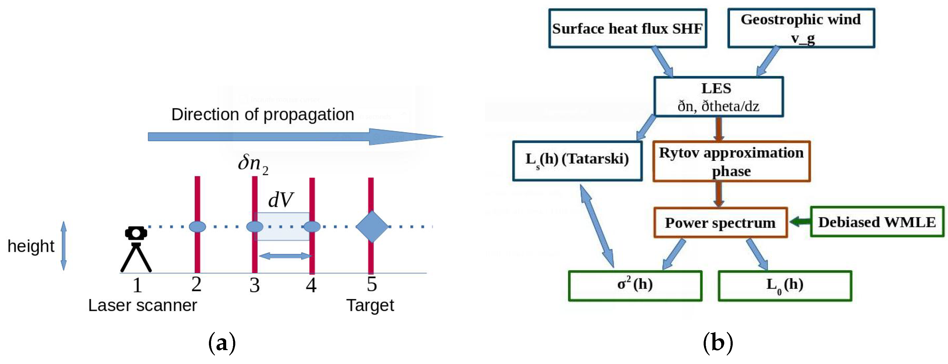
Figure 2.
Average height profiles for case 1: mixed turbulence (a) left: potential temperature in K, middle: resolved vertical turbulent sensible heat flux, right: horizontal momentum flux. (b) left: vertical momentum flux, middle: anisotropy factor, right: v-component of the velocity.
Figure 2.
Average height profiles for case 1: mixed turbulence (a) left: potential temperature in K, middle: resolved vertical turbulent sensible heat flux, right: horizontal momentum flux. (b) left: vertical momentum flux, middle: anisotropy factor, right: v-component of the velocity.
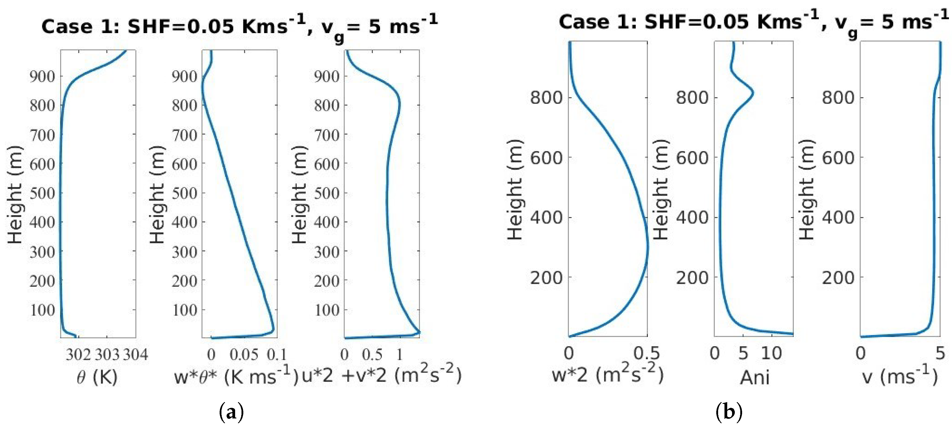
Figure 3.
Profiles of (a) (red) and (Masciadri, blue) with height (m) starting from 100 m for the three cases under consideration, (b) cutoff , (c) R defined as the ratio and (d) , x-axis: log10 plot.
Figure 3.
Profiles of (a) (red) and (Masciadri, blue) with height (m) starting from 100 m for the three cases under consideration, (b) cutoff , (c) R defined as the ratio and (d) , x-axis: log10 plot.
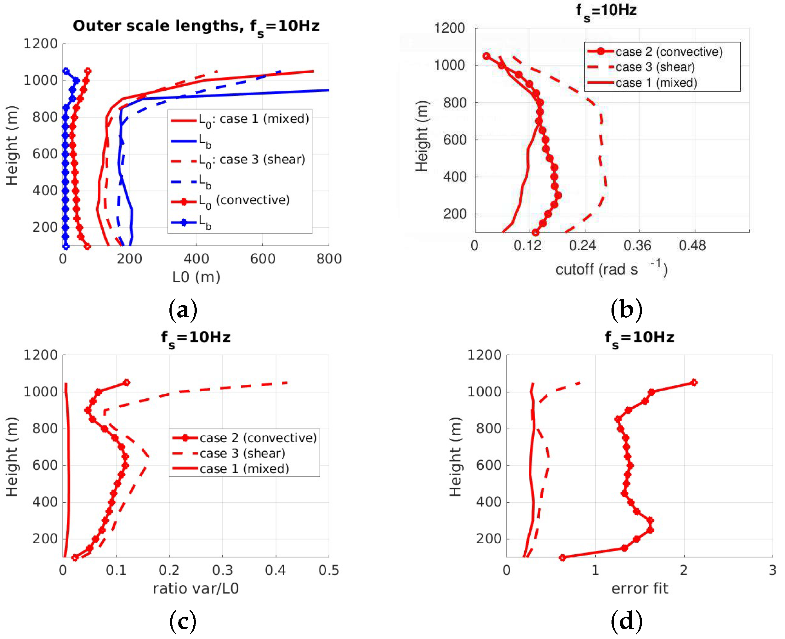
Figure 4.
Phase diagnostic for case 1: (a) probability density function of at different heights (b) the corresponding time series, shifted for the sake of readability.
Figure 4.
Phase diagnostic for case 1: (a) probability density function of at different heights (b) the corresponding time series, shifted for the sake of readability.
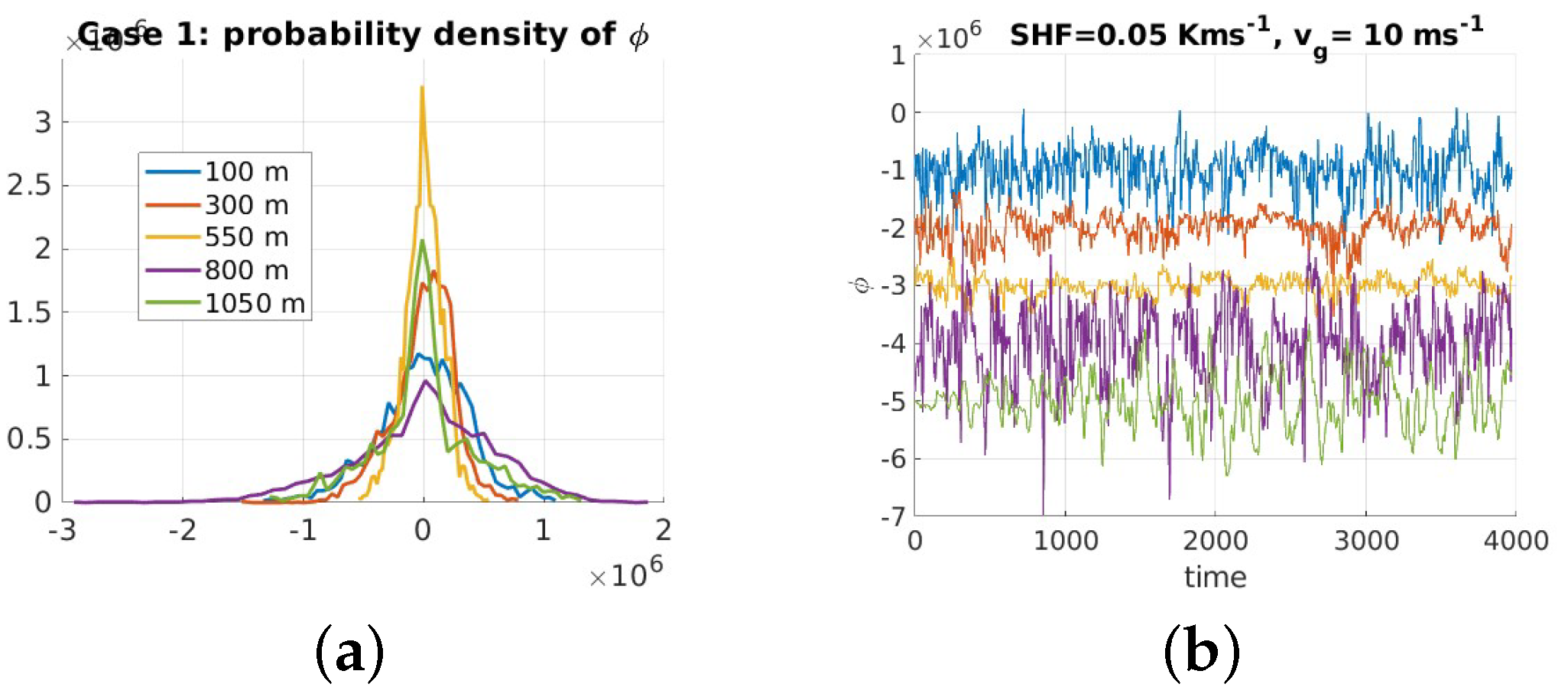
Figure 5.
Average profiles for case 3: shear-driven turbulence, see Figure 2 for caption description.
Figure 5.
Average profiles for case 3: shear-driven turbulence, see Figure 2 for caption description.

Figure 6.
Average profiles for case 3: shear-driven turbulence, see Figure 2 for caption description.
Figure 6.
Average profiles for case 3: shear-driven turbulence, see Figure 2 for caption description.

Figure 7.
Profiles with height of (a), (b) and R (c) for cases 1–3 following the LES setups described in Table 1.
Figure 7.
Profiles with height of (a), (b) and R (c) for cases 1–3 following the LES setups described in Table 1.


Table 1.
LES setups.
| Case | (K m s−1) | (m s−1) | Description |
|---|---|---|---|
| 1 | 0.05 | 5 | mixed: shear + buoyancy |
| 2 | 0.1 | 1 | buoyancy |
| 3 | 0.05 | 10 | shear |
Disclaimer/Publisher’s Note: The statements, opinions and data contained in all publications are solely those of the individual author(s) and contributor(s) and not of MDPI and/or the editor(s). MDPI and/or the editor(s) disclaim responsibility for any injury to people or property resulting from any ideas, methods, instructions or products referred to in the content. |
© 2024 by the author. Licensee MDPI, Basel, Switzerland. This article is an open access article distributed under the terms and conditions of the Creative Commons Attribution (CC BY) license (https://creativecommons.org/licenses/by/4.0/).
Share and Cite
MDPI and ACS Style
Kermarrec, G. On a Correlation Model for Laser Scanners: A Large Eddy Simulation Experiment. Remote Sens. 2024, 16, 3545. https://doi.org/10.3390/rs16193545
AMA Style
Kermarrec G. On a Correlation Model for Laser Scanners: A Large Eddy Simulation Experiment. Remote Sensing. 2024; 16(19):3545. https://doi.org/10.3390/rs16193545
Chicago/Turabian StyleKermarrec, Gaël. 2024. "On a Correlation Model for Laser Scanners: A Large Eddy Simulation Experiment" Remote Sensing 16, no. 19: 3545. https://doi.org/10.3390/rs16193545
Note that from the first issue of 2016, this journal uses article numbers instead of page numbers. See further details here.