Opposing Impacts of Greenspace Fragmentation on Land Surface Temperature in Urban and Surrounding Rural Areas: A Case Study in Changsha, China

Abstract

Managing the amount of greenspace (i.e., increasing or decreasing greenspace coverage) and optimizing greenspace configuration (i.e., increasing or decreasing greenspace fragmentation) are cost-effective approaches to cooling the environment. The spatial variations in their impacts on the thermal environment, as well as their relative importance, are of great importance for greenspace planning and management but are far from thoroughly understood. Taking Changsha, China as an example, this study investigated the spatial variations of the impacts of greenspace amount (measured as a percent of greenspace) and greenspace fragmentation (measured by edge density of greenspace) on the Landsat-derived land surface temperature (LST) using geographically weighted regression (GWR), and also uncovered the spatial pattern of their relative importance. The results indicated that: (1) Greenspace amount showed significantly negative relationships with LST for 91.29% of the study area. (2) Both significantly positive and negative relationships were obtained between greenspace fragmentation and LST, covering 14.90% and 13.99% of the study area, respectively. (3) The negative relationship between greenspace fragmentation and LST is mainly located in the urban areas, while the positive relationship appeared in the rural areas. (4) Greenspace amount made a larger contribution to regulating LST than greenspace fragmentation in 93% of the study area, but the latter had stronger roles in about 6.95% of the study area, mainly in the city center. These findings suggest that spatially varied greenspace planning and management strategies should be adopted to improve the thermal environment.

1. Introduction

Urban and surrounding rural areas are experiencing rapid temperature increases caused by both global warming and the urban heat island effect [1,2,3], and thus are suffering from severe ecological and environmental consequences, such as increasing building cooling energy use [4], threatening biodiversity [5], risking human health [6]. Mitigation of the elevating temperature has attracted increasing attention from both scientific communities and decision-makers, as more than half the global population resides here [7,8]. Several strategies—such as land greening (e.g., increasing greenspace coverage, building green roofs) [9], land evaporation (e.g., increasing water coverage, installing spray fountains) [10], increasing albedo through white rooftops and light-colored pavements [11], and constructing urban ventilation corridors [12]—have been widely suggested and effectively adopted to decrease urban temperature [13]. Greenspace, the landscape that is covered with vegetation in the form of trees, shrubs, and grasses can significantly decrease temperature because: (1) it has strong evapotranspiration, which can absorb solar radiation and transfer sensible heat to latent heat [14,15,16]; (2) it can generate a large amount of shadow, which prevents the surface from direct heating by solar radiation [17,18,19]; and (3) it has a higher albedo compared to the developed impervious surfaces of buildings, for example [20,21]. A proliferation of studies demonstrate a significant negative relationship between temperature and the strategy of planting more trees, and this has been recognized and applied as a cost-effective, nature-based solution to mitigate temperature increase [22,23].

Though expanding greenspace coverage by, for example, planting more trees is theoretically effective in decreasing urban temperature, it is very difficult if not impossible in practice because land for greening is usually limited, especially in highly developed urban areas. Based on the landscape ecology theory, greenspace in any area is formed by several patches with different sizes and shapes, which generate different spatial compositions (i.e., the amount of greenspace) and spatial configuration (i.e., fragmentation, aggregation). Spatial composition and also the spatial configuration of greenspace both significantly impact energy flow and the consequent temperature [24,25,26]. Researchers also found that the spatial configuration of greenspace even had a stronger impact on surface temperature than the spatial composition of greenspace [27,28]. Therefore, optimizing the spatial configuration of the greenspace is another effective approach to mitigate temperature increase in addition to expanding the greenspace area.

Fragmentation is a fundamental characteristic of landscape configuration [29,30,31] and greenspace fragmentation has been widely demonstrated as an important factor impacting surface temperature [27,32,33]. Current studies among different cities showed diverse and even opposite results. For example, some studies reported significant negative relationships between greenspace fragmentation and surface temperature [34,35], while others concluded that there were positive impacts of greenspace fragmentation [24,36]. Many studies showed that greenspace amount has a stronger impact than greenspace fragmentation [32,33,37], but other studies reported a stronger impact of greenspace fragmentation than greenspace amount [27,28]. Furthermore, the impact of greenspace fragmentation on temperature and its relative importance compared to greenspace amount also showed strong intra-city variations. For example, Guo et al. showed that greenspace amount dominated the drivers of LST in Guangzhou and Shenzhen, China, but greenspace fragmentation also explained more variation of LST in some other areas [38].

Previous investigations of the impact of greenspace fragmentation on temperature mostly assume a spatially consistent relationship between them, and the global least squares regression was applied [39,40]. This approach has the limitation of decreasing the prediction power, hindering the spatial variation of the impacts [38,41]. Geographically weighted regression (GWR) is an effective approach and has been widely adopted to investigate the spatial non-stationarity of the relationships between landscape patterns and ecological processes [42]. Some studies have applied GWR to investigate the spatial variations of the relationship between LST and land indicators (such as land cover fraction, vegetation index, land use intensity, etc.) [41,43,44]. However, few studies have uncovered the spatial variations of the impacts of greenspace amount and greenspace fragmentation, as well as their relative importance.

Taking the subtropic city of Changsha, China as an example, this study aims to investigate the spatial variation of greenspace fragmentation impacts on surface temperature. We attempted to answer two questions: (1) How does the relationship between greenspace fragmentation and LST vary spatially? (2) How does the relative contribution of greenspace amount and greenspace fragmentation on LST vary spatially? We built geographically weighted regression (GWR) with Landsat LST as the dependent variable and greenspace fragmentation (i.e., edge density) as well as percent land covers (i.e., cropland, bare land, and greenspace) and elevation as independent variables. Variance partitioning was applied to investigate the relative importance of greenspace amount and greenspace fragmentation to explain the variation of LST. The findings of this study can extend our understanding of the spatial variations of the greenspace fragmentation impacts on LST and aid better urban greenspace planning and management.

2. Materials and Methods

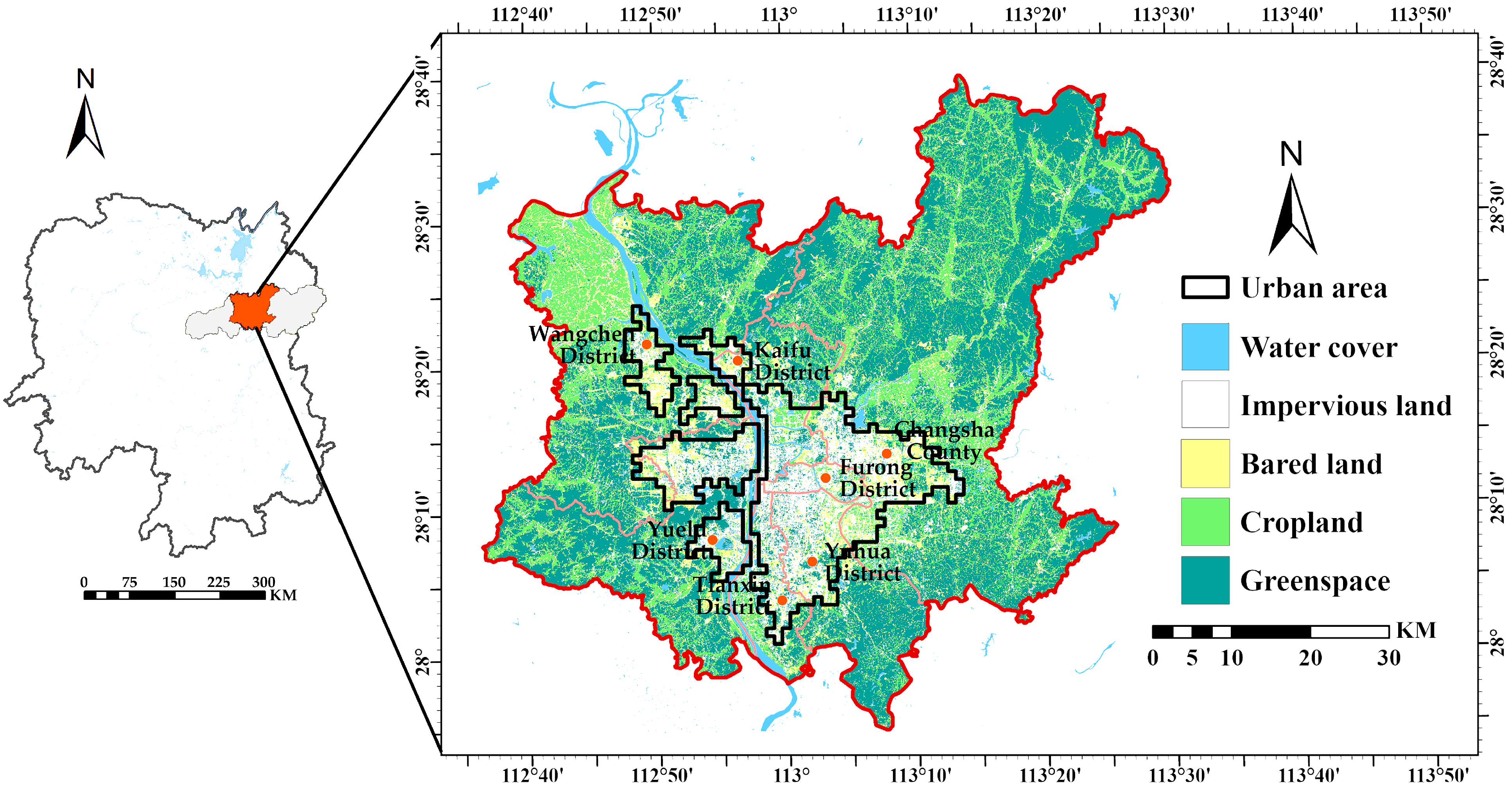
2.1. Study Area

Changsha (111°53′~114°E, 27°51′~28°41′N), the capital city of Hunan Province, is situated in the northeastern part of Hunan Province, China (Figure 1). It lies along the lower reaches of the Xiang River and the western edge of the Changliu Basin. The city has elevations ranging from 23.5 to 1607.9 m. Changsha has a subtropical monsoon climate, characterized by hot summer and cold winter. In 2020, the city recorded an annual average temperature of 18.2 °C [45].

Changsha has experienced rapid urban expansion and socioeconomic development since 1978. The urbanization rate increased from 20.5% to 82.60%, and GDP soared from 16.85 billion RMB to 1214.252 billion RMB [45]. During urbanization, large areas of farmland were transformed into impervious surfaces, as part of urban development, causing the thermal environment in downtown Changsha to heat up each year. The proportion of high-temperature areas has continuously increased, and the urban heat island effect has intensified. Rapid urbanization has also shifted the spatial distribution of heat islands from concentrated urban zones to a more dispersed, multi-center pattern, making the urban heat island effect increasingly prominent. Our study area encompasses seven districts (i.e., Furong District, Yuelu District, Yuhua District, Tianxin District, Kaifu District, Wangcheng District, and Changsha County) (Figure 1). Water was excluded within the study area in later analyses, to avoid its impact on temperature.

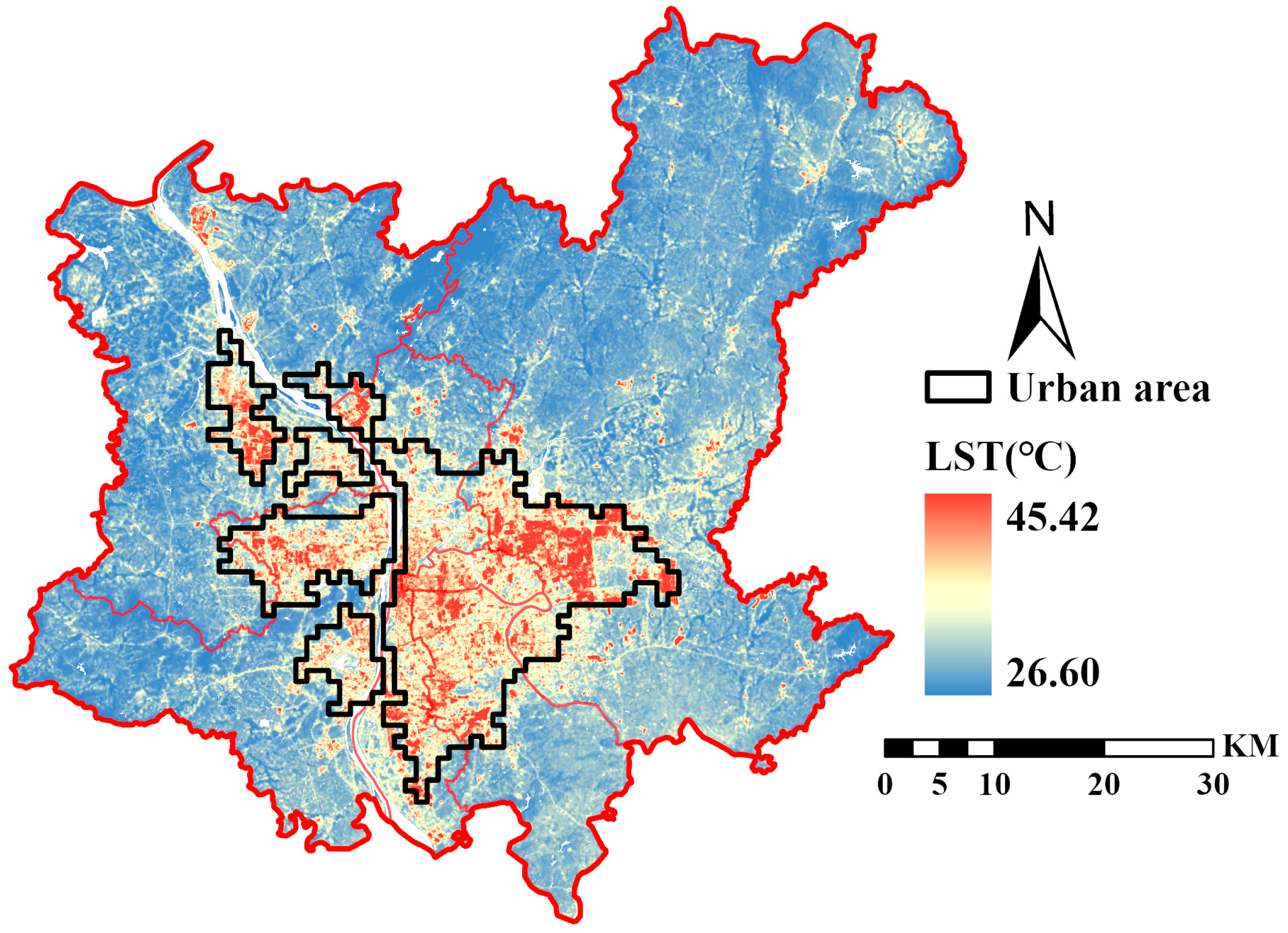
2.2. Land Surface Temperature

We employed Landsat-8 OLI TIRS satellite data (Collection 1, Level 1, LANDSAT/LC08/C01/T1_SR) downloaded from the United States Geological Survey (https://earthexplorer.usgs.gov/, accessed on 20 April 2024) to retrieve LST. Based on data availability, we selected LST data on 17 August 2019, a typical clear sky day in the hot summer with an average temperature of 32.50 °C (29–37 °C), an average wind speed of 1.47 m/s, and an average humidity of 60.13%. The LST was derived using the radiative transfer equation method [46,47,48].

$$\mathrm{LST}={\displaystyle \frac{{\mathrm{T}}_{\mathrm{B}}}{1+\left(\frac{{\mathsf{\lambda }\mathrm{T}}_{\mathrm{B}}}{\rho }\right)\ast \ln \left(\mathsf{\epsilon }\right)}}$$

(1)

where ${\mathrm{T}}_{\mathrm{B}}$ is brightness temperature which is estimated by the following Equation (2) and $\mathsf{\lambda }$ is the central wavelength of the thermal infrared band (i.e., 10.9). $\rho$= 1.438 × 10⁻² mk. ε is the surface emissivity, which is estimated by the following Equation (3).

The radiance of the thermal infrared band (B10) was converted to brightness temperature ${\mathrm{T}}_{\mathrm{B}}$.

$${\mathrm{T}}_{\mathrm{B}}={\displaystyle \frac{{\mathrm{K}}_2}{\ln \left({\mathrm{K}}_1/{\mathrm{L}}_{\mathsf{\lambda }}+1\right)}}$$

(2)

where ${\mathrm{L}}_{\mathsf{\lambda }}$ is the the radiance of the thermal infrared band (B10) and ${\mathrm{K}}_1$ and ${\mathrm{K}}_2$ are preset constants before launch. ${\mathrm{K}}_1$ = 1321.08 and ${\mathrm{K}}_2$ = 774.89.

$$\mathsf{\epsilon }=\left\{\begin{array}{c}0.004\ast {\mathsf{\rho }}_{\mathrm{Red}}+0.979 \left(\mathrm{NDVI}<0.2\right)\\ 0.987 \ast {\mathrm{P}}_{\mathrm{v}}+0.971\ast \left(1-{\mathrm{P}}_{\mathrm{v}}\right) \left(0.2\le NDVI\le 0.5\right)\\ 0.987 \left(0.5<\mathrm{NDVI}\right)\end{array}\right.$$

(3)

where ${\mathrm{P}}_{\mathrm{v}}$ is vegetation fraction and was derived using Equation (4) [49]. ${\mathsf{\rho }}_{\mathrm{Red}}$ is Landsat-8 band 4 (Red).

$${\mathrm{P}}_{\mathrm{v}}={\left({\displaystyle \frac{\mathrm{NDVI}-{\mathrm{NDVI}}_{\min }}{{\mathrm{NDVI}}_{\max }-{\mathrm{NDVI}}_{\min }}}\right)}^2$$

(4)

where NDVI is the normalized difference vegetation index [50] calculated using the surface reflectance of Landsat-8 band 4 (Red) and band 5 (NIR), as shown in Equation (5).

$$\mathrm{NDVI}={\displaystyle \frac{\left({\mathsf{\rho }}_{\mathrm{NIR}}-{\mathsf{\rho }}_{\mathrm{Red}}\right)}{\left({\mathsf{\rho }}_{\mathrm{NIR}}+{\mathsf{\rho }}_{\mathrm{Red}}\right)}}$$

(5)

Figure 2 shows the spatial distribution of LST in the study area. We quantified the average LST for each 1 km grid (the analytical unit), which is used as the dependent variable in later statistical analysis.

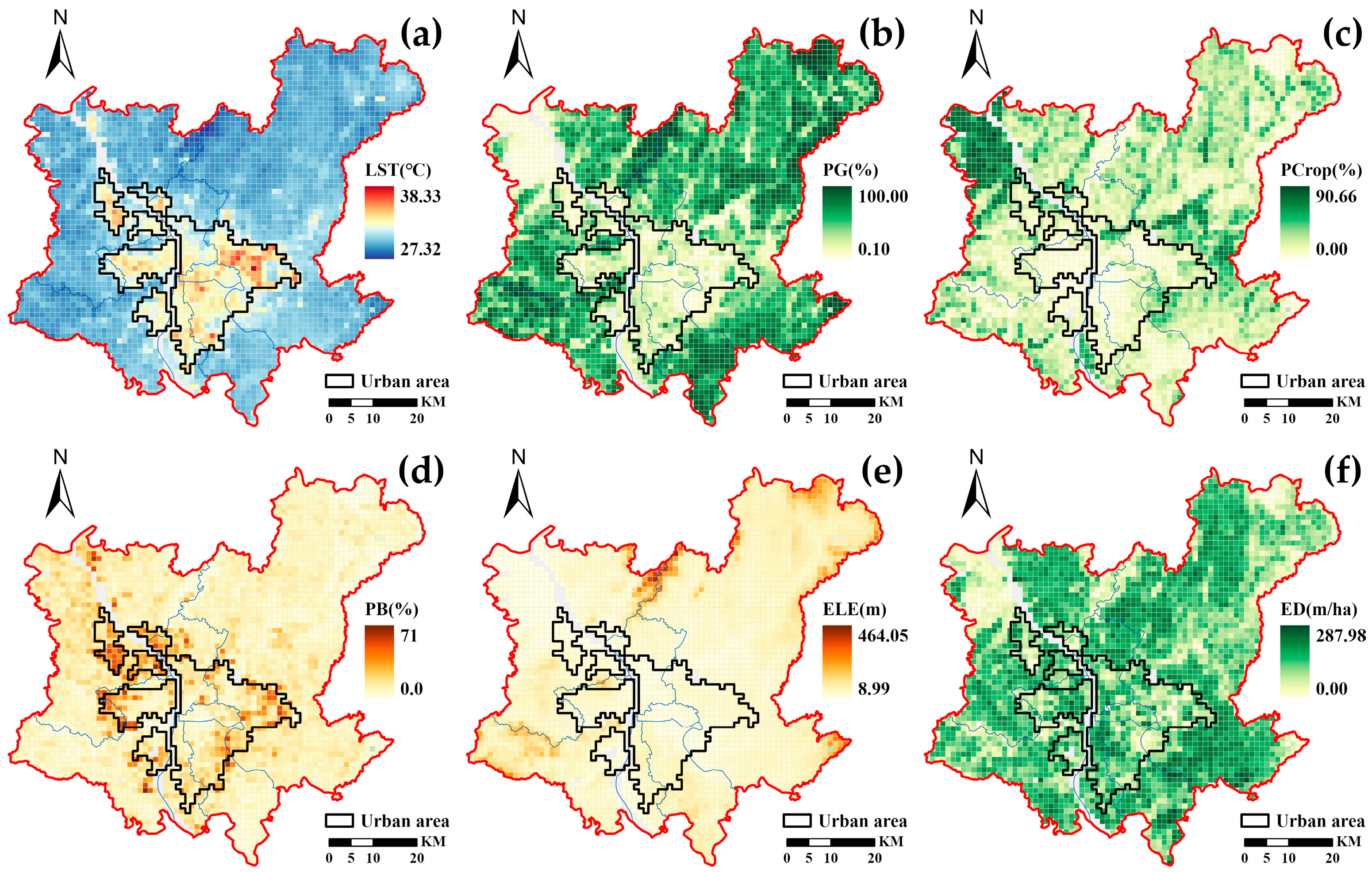
2.3. Quantifying Landscape Composition and Greenspace Fragmentation

We quantified landscape composition (i.e., percent of land cover) for each 1 km grid using Equation (6).

$${\mathrm{P}}_{\mathrm{i}}={\displaystyle \frac{{\mathrm{S}}_{\mathrm{i}}}{\mathrm{A}}}\ast 100\%$$

(6)

where ${\mathrm{P}}_{\mathrm{i}}$ is the percent of land cover i (i.e., greenspace, cropland, and bare land), ${\mathrm{S}}_{\mathrm{i}}$ is the total area of land cover, and $\mathrm{A}$ is the area of the analytical unit (i.e., the 1 km grid).

Following previous studies [33,51], we quantified the edge density of greenspace to measure its fragmentation using Equation (7).

$$\mathrm{E}\mathrm{D}=\frac{\sum _{\mathrm{k}=1}^{\mathrm{m}} {\mathrm{e}}_{\mathrm{k}}}{\mathrm{A}}\ast 10000$$

(7)

where ${\mathrm{e}}_{\mathrm{k}}$ is the edge length of the kth greenspace patch in meters, m is the total number of greenspace patches, and $\mathrm{A}$ is the size of the unit (i.e., the 1 km grid). The increase in edge density is a fundamental process of landscape fragmentation and a higher value indicates a greater degree of fragmentation [52,53,54]. Both landscape composition and greenspace fragmentation were calculated using the “landscapemetrics” package of R 4.4.1 [55].

2.4. Statistical Analysis

We built a multiple linear regression model to investigate the impact of land cover and greenspace fragmentation on LST. The regression model was specified as Equation (8).

$$\mathrm{y}={\mathsf{\beta }}_0+{{\displaystyle \sum }}_{\mathrm{k}=1}^{\mathrm{m}}{\mathsf{\beta }}_{\mathrm{k}}{\mathrm{x}}_{\mathrm{k}}+ϵ$$

(8)

where ${\mathsf{\beta }}_0$ is the intercept, ${\mathsf{\beta }}_{\mathrm{k}}$ are the regression coefficients for explanatory variable k (i.e., percent of greenspace, percent of cropland, percent of bare land, elevation, and greenspace fragmentation), and $\mathsf{ϵ}$ is the random error. These regression coefficients were estimated using the ordinary least squares (OLS) algorithm, which assumes spatially consistent linear relationships between LST and the explanatory variables. Variance inflation factors of the five explanatory variables are lower than 5, suggesting the model is not suffering from multicollinearity.

We applied GWR to investigate the spatial variation of the impacts of these explanatory variables on LST. GWR performs a local regression for each place (grid, site) based on samples surrounding it, so for each grid it generates spatially varied regression coefficients, significance, and R² [41]. The GWR model was specified as Equation (9).

$${\mathrm{y}}_{\mathrm{i}}={\mathsf{\beta }}_0\left({\mathrm{u}}_{\mathrm{i}},{\mathrm{v}}_{\mathrm{i}}\right)+{{\displaystyle \sum }}_{\mathrm{k}=1}^{\mathrm{m}}{\mathsf{\beta }}_{\mathrm{k}}\left({\mathrm{u}}_{\mathrm{i}},{\mathrm{v}}_{\mathrm{i}}\right){\mathrm{x}}_{\mathrm{ik}}+{\mathsf{\epsilon }}_{\mathrm{i}}$$

(9)

where ${\mathrm{y}}_{\mathrm{i}},{ \mathrm{x}}_{\mathrm{ik}},{ \mathsf{\epsilon }}_{\mathrm{i}}$ represent the dependent variable, the independent variables, and random error at location $\mathrm{i}$. ${\mathsf{\beta }}_0\left({\mathrm{u}}_{\mathrm{i}},{\mathrm{v}}_{\mathrm{i}}\right)$ is the geographically varying intercept and ${\mathsf{\beta }}_{\mathrm{k}}\left({\mathrm{u}}_{\mathrm{i}},{\mathrm{v}}_{\mathrm{i}}\right)$ represents the local regression coefficients for the kth explanatory variable at location i.${ \mathsf{\epsilon }}_{\mathrm{i}}$ is the random error at location $\mathrm{i}$. The coordinates $\left(\mathrm{ui},\mathrm{vi}\right)$ indicate the spatial location of location $\mathrm{i}$. We employed an adaptive Gaussian kernel function and selected the optimal bandwidth based on the Cross-Validation [56]. We calculated the coefficient of determination (R²), spatial autocorrelation of the residuals, and Akaike Information Criterion for both OLS and GWR. The “spgwr” package in R was utilized to fit the GWR model.

We applied variance partitioning to assess the relative importance of greenspace amount and greenspace configuration in explaining the variation of LST [32,33]. We categorized the explanatory variables as those included in the GWR model into three groups: greenspace amount (i.e., percent of greenspace), greenspace fragmentation (i.e., edge density of greenspace), and other variables (i.e., percent of cropland, percent of bare land, and elevation). We fitted a series of GWR models with different combinations of these three groups of variables and partitioned the predicted variation of LST (R²) into independent effects and joint effects of these three groups of variables using the variance partitioning method. The details of the variance partitioning process can be found in [32,57].

3. Results

3.1. Descriptive Statistics

The average LST is 30.47 °C (27.32–38.33 °C), with a standard deviation of 1.45 °C (

Table 1. Descriptive statistics of percent land cover, edge density, and LST at the 1 km grid level.

Variables (Unit)	Mean	SD	Min	Max
LST (°C)	30.468	1.448	27.316	38.334
Percent of greensapce (%)	49.073	28.252	0.102	100.00
Percent of cropland (%)	24.161	19.394	0.00	90.658
Percent of bare land (%)	12.085	9.605	0.00	71.092
Elevation (m)	59.478	44.2	8.986	464.05
Edge density of greenspace (m·hm−2)	136.752	59.651	0.00	287.979

). The urban area shows very high LST as a big island compared with the rural areas (Figure 3a). The average percent of greenspace is 49.073% (0.10–100%). The urban area has lower values, with some scattered hotspots such as urban parks; and the rural area has a high coverage of greenspace (Figure 3b). The average percent of cropland is 24.16% (0–90.658%), which is primarily concentrated in the northwestern regions and middle east of the study area (Figure 3c). The average percent of bare land is 12.09% (0–71.09%), mainly distributed in the fringe of the urban areas (Figure 3d). The average edge density of greenspace is 136.75 m·hm⁻² (0–287.98 m·hm⁻²). The spatial distribution of edge density of greenspace did not show a clear urban–rural difference (Figure 3f).

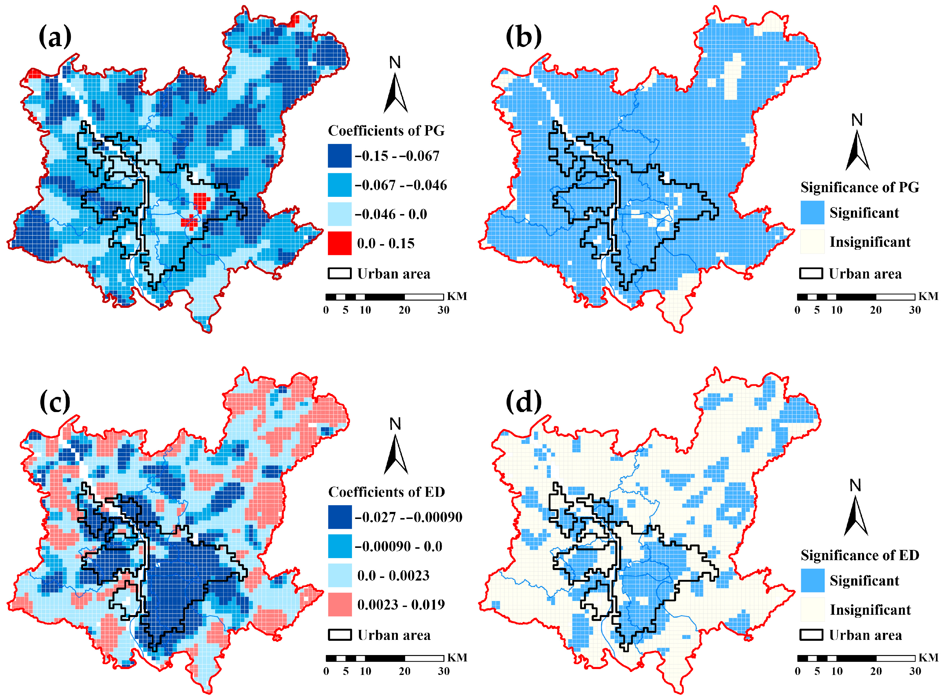
3.2. Spatial Variation of Greenspace Fragmentation Impacts on LST

The OLS model explained 86.79% of the variation of LST (

Table 2. Summary of the OLS model and GWR model.

Factors	OLS				GWR
	Estimate	Std. Error	t Value	VIF	Mean	Min	1st Qu	3rd Qu	Max
(Intercept)	35.17 ***	0.057	617.11	/	35.25	25.84	34.22	36.28	45.77
PG	−0.055 ***	0.00060	−94.28	3.11	−0.056	−0.15	−0.067	−0.046	0.15
PC	−0.021 ***	0.0013	−16.26	1.62	−0.061	−0.16	−0.073	−0.048	0.029
PB	−0.064 ***	0.00060	−104.76	1.72	−0.033	−0.20	−0.047	−0.017	0.090
ED	0.00030	0.00020	1.79	1.37	0.00030	−0.027	−0.00090	0.0023	0.019
ELE	−0.0041 ***	0.00030	−12.21	2.49	0.0011	−0.073	−0.0062	0.0039	0.13
R-squared	0.87				0.98
Diagnostics		OLS			GWR
Residual sum of squares		875.55			139.93
log Lik		−2457.89			1201.22
Classic AIC		4929.79			−12.38
AICc		4929.82			1547.36
Adjusted R-squared:		0.87			0.97
Moran’s I		0.67 ***			0.0047

ED is edge density, ELE is elevation, PG, PC, PB are percent of greenspace, percent of cropland, and percent of bare land, respectively. *** p <= 0.001.

). Percent of greenspace, percent of bare land, percent of cropland, and elevation show a significant negative regression coefficient; while the edge density of greenspace displays an insignificant positive value (Table 2). The residual of the OLS model shows significant spatial autocorrelation with a Moran’s I of 0.67 (p < 0.01). The GWR model explained 96.61% of the variation of LST (Table 2). The local R² showed strong spatial variations ranging from 0.665 to 0.998 (Figure 4a). Only 6.95% of the study area had R² lower than 0.90, mainly located in the northeast, central, and southwest of the rural areas (Figure 4b). The spatial autocorrelation of the residual of the GWR model is not significant with a Moran’s I of 0.0047 (p > 0.05).

Regression coefficients of the percent of greenspace showed an average of −0.056, ranging from −0.151 to 0.152 (Table 2). This indicates that every 10% increase of greenspace coverage in each 1 km grid can averagely decrease LST by 0.56 °C. However, this value had strong spatial variations, with LST decreasing as much as 1.51 °C or increasing as much as 1.52 °C. Expanding greenspace coverage can decrease LST in 98.77% of the study area where the regression coefficient had a negative value (Figure 5a). Specifically, 91.29% of the study area showed significant negative values, demonstrating that expanding greenspace coverage in these areas can effectively decrease LST (Figure 5b). Areas with a strong cooling effect of greenspace expansion (i.e., regression coefficient lower than −0.06) were mainly distributed in the rural areas (Figure 5a).

Regression coefficients of greenspace fragmentation showed an average of 0.0003, ranging from −0.029 to 0.019 (Table 2). This indicates that every unit increase of greenspace fragmentation can, on average, increase LST by 0.003 °C. However, this value had strong spatial variations, with LST decreasing as high as 0.29 °C or increasing as high as 0.19 °C. Greenspace fragmentation can decrease LST in 36.47% of the study area where the regression coefficient had a negative value (Figure 5c). Specifically, 13.99% of the study area showed significant negative values, demonstrating that increasing greenspace fragmentation in these areas can effectively decrease LST (Figure 5d). Greenspace fragmentation will increase LST in 64.53% of the study area, as the regression coefficient is positive (Figure 5c). Specifically, 14.90% of the study areas showed significant positive values, indicating that enhancing greenspace fragmentation in these areas can effectively increase LST (Figure 5d). Almost all the urban areas showed significant negative regression coefficients of greenspace fragmentation, while the positive values were scattered in the rural areas (Figure 5c).

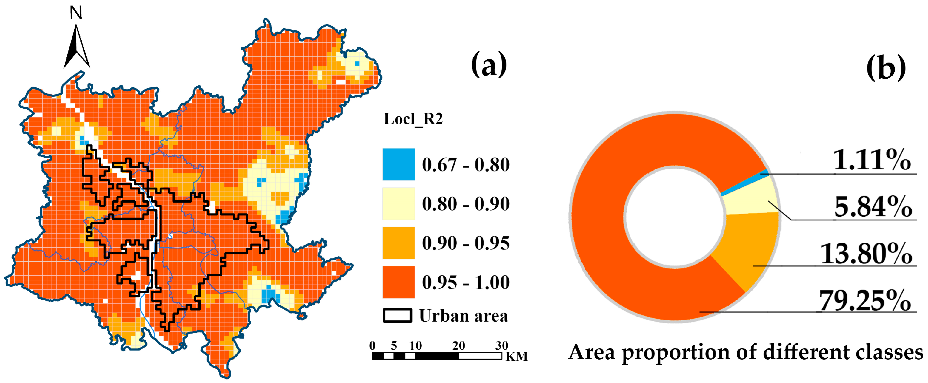
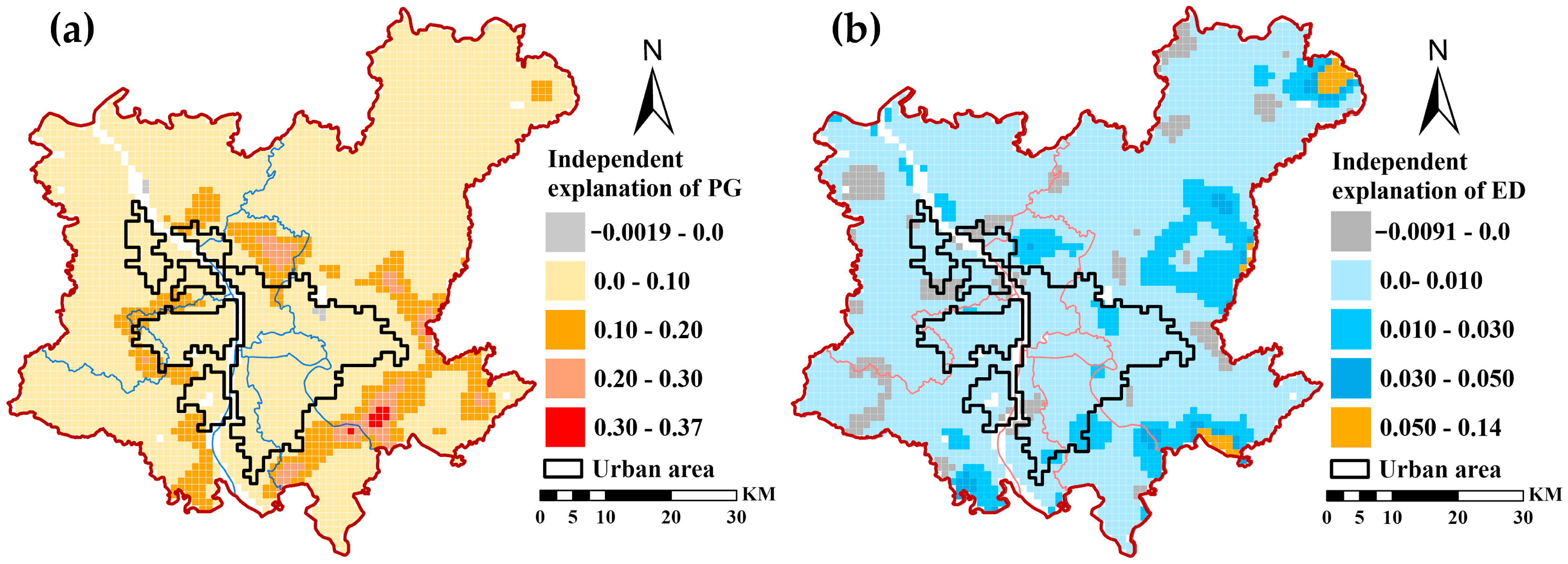
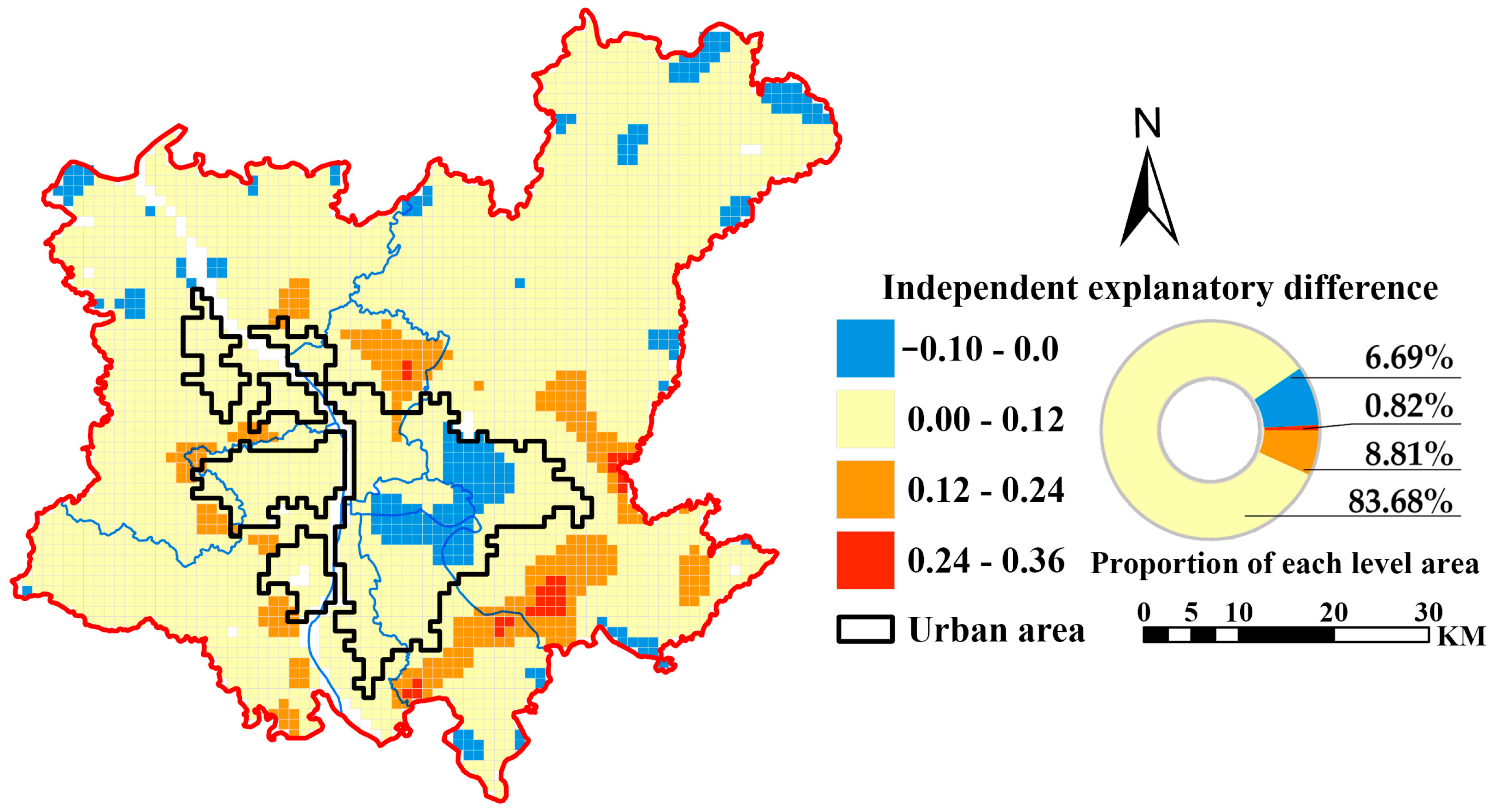
3.3. Spatial Variation of the Relative Importance of Greenspace Coverage and Fragmentation

Greenspace amount independently explained 4.64% of the LST variations, ranging from −0.19% to 37%. The independent explanation of greenspace amount showed strong spatial variations with the high values (i.e., that higher than 10%) located in the suburban area near the urban areas (Figure 6a). Greenspace fragmentation independently explained 0.54% of the LST variations, ranging from −0.91% to 14% (Figure 6b). Most regions show low individual contributions from ED, with a few high values occurring in the northeast and southeast of the city.

Figure 7 shows the difference of the independently explained variance of LST by greenspace amount and greenspace fragmentation. The positive values mean a stronger impact of greenspace amount than greenspace fragmentation and vice versa. Greenspace amount displays stronger impacts on LST than greenspace fragmentation in about 93% of the study area. The city center and sub-center in the east of the study area witnessed a stronger impact of greenspace fragmentation than greenspace amount.

4. Discussion

4.1. Spatial Variation of the Greenspace Fragmentation Impacts on LST

According to previous research, greenspace fragmentation impacts LST through two approaches: altering evapotranspiration and changing the amount of shadow [17,58,59]. Increasing greenspace fragmentation usually decreases evapotranspiration but increases shadow, and thus generates opposite effects on temperature. Therefore, the direction of the greenspace fragmentation impacts on LST is a tradeoff between these two energy processes [28,60,61].

The regression coefficients of greenspace edge density show strong spatial variations with nearly equal areas of significant positive and negative values. Strong spatial variations of the regression coefficient between surface temperature and landscape configuration metrics were also reported in previous studies. For example, LST and land cover diversity measured by Shannon’s diversity showed both significant positive and negative relationships in Austin and San Antonio, Texas, USA [43]. Regression coefficients of patch richness density for different land covers in explaining the variation of LST ranged from negative to positive in Shenzhen, China [41]. The GWR model reported both positive and negative regression coefficients for landscape metrics (i.e., patch density, aggregation index, and largest patch index) using LST as the dependent variable in Dalian, China [44]. The spatial variation of the relationship between surface temperature and landscape configuration metrics was possibly caused by the significant spatial variations in, for example, land use and land cover, landscape structure, development intensity, vegetation type, anthropogenic heat release, and so on [28,37,62,63].

The spatial distribution of the regression coefficients of greenspace edge density shows clear urban and rural differences, with negative values in the almost urban areas and positive values in the almost rural areas. This indicates that fragmented greenspace in the urban areas can decrease LST, while that in the rural areas will increase LST. In highly developed urban areas where impervious surface dominates the landscape, evapotranspiration is reduced [64]. Increasing greenspace edge density generates more shadow to cool the environment, but decreases evapotranspiration. The increased cooling effect from shadow generated by greenspace fragmentation overpasses the lost evapotranspiration cooling effect, and thus a significant negative relationship was observed between LST and greenspace fragmentation [65,66]. In the less developed rural areas where vegetation (i.e., forest and crop) dominantly covers the landscape, strong evapotranspiration dominates the energy process. The shadow-generated cooling can be ignored in the rural area and it may even decrease the evapotranspiration of vegetation in the shadow. Therefore, greenspace fragmentation in rural areas may decrease the cooling effect of the landscape and result in a positive relationship between LST and greenspace fragmentation.

4.2. Management Implementations

Our study showed that greenspace amount has a stronger role in regulating LST than greenspace fragmentation. This suggests that managing greenspace amount (i.e., increasing greenspace coverage) is more effective than optimizing greenspace fragmentation to mitigate temperature increase. Considering the dominance of impervious surfaces in urban areas and the increasing importance of farmland in rural areas, it is not possible to expand greenspace without limitation. Greening impervious surfaces such as roofs and walls can be adopted to increase greenspace amount in highly developed urban areas. In rural areas, farmland shelter belts composed of trees can be well designed to enhance their cooling effects.

The significant but spatially varied impact of greenspace fragmentation on LST suggests that optimizing spatial configuration (i.e., fragmentation) of greenspace can effectively improve the thermal environment. Furthermore, the relationships between LST and greenspace fragmentation were opposite between urban and rural areas. This suggests that the traditional “one-size-fits-all” strategy is not applicable and a spatially explicit greenspace fragmentation optimization strategy should be developed. Specifically in urban areas, increasing greenspace fragmentation besides expanding greenspace coverage should be considered and, in the rural areas, decreasing greenspace fragmentation should be recommended.

5. Conclusions

This study investigated the spatial variations of the impacts of greenspace amount and greenspace fragmentation on LST using geographically weighted regression. Generally, greenspace amount contributed more than greenspace fragmentation to regulating LST. Expanding greenspace coverage can effectively decrease LST for the whole study area, but the impacts of greenspace fragmentation on LST varied spatially and even showed opposite impacts between urban and surrounding rural areas. Specifically, greenspace fragmentation positively impacted LST in rural areas, but negatively impacted LST in urban areas. We also found that in the highly developed urban center, greenspace fragmentation has a stronger role in explaining the variation of LST than greenspace fragmentation. Our study suggests spatially explicit urban greenspace planning and management strategies to improve the thermal environment.

References

1. Yang, M.; Ren, C.; Wang, H.; Wang, J.; Feng, Z.; Kumar, P.; Haghighat, F.; Cao, S.-J. Mitigating urban heat island through neighboring rural land cover. Nat. Cities 2024, 1, 522–532. [Google Scholar] [CrossRef]
2. Chen, J.; Zhan, W.; Du, P.; Li, L.; Li, J.; Liu, Z.; Huang, F.; Lai, J.; Xia, J. Seasonally disparate responses of surface thermal environment to 2D/3D urban morphology. Build. Environ. 2022, 214, 108928. [Google Scholar] [CrossRef]
3. Chen, J.; Zhan, W.; Jin, S.; Han, W.; Du, P.; Xia, J.; Lai, J.; Li, J.; Liu, Z.; Li, L.; et al. Separate and combined impacts of building and tree on urban thermal environment from two- and three-dimensional perspectives. Build. Environ. 2021, 194, 107650. [Google Scholar] [CrossRef]
4. Li, X.; Zhou, Y.; Yu, S.; Jia, G.; Li, H.; Li, W. Urban heat island impacts on building energy consumption: A review of approaches and findings. Energy 2019, 174, 407–419. [Google Scholar] [CrossRef]
5. Habibullah, M.S.; Din, B.H.; Tan, S.-H.; Zahid, H. Impact of climate change on biodiversity loss: Global evidence. Environ. Sci. Pollut. Res. 2021, 29, 1073–1086. [Google Scholar] [CrossRef] [PubMed]
6. Mora, C.; Dousset, B.; Caldwell, I.R.; Powell, F.E.; Geronimo, R.C.; Bielecki, C.R.; Counsell, C.W.W.; Dietrich, B.S.; Johnston, E.T.; Louis, L.V.; et al. Global risk of deadly heat. Nat. Clim. Chang. 2017, 7, 501–506. [Google Scholar] [CrossRef]
7. Yu, Z.; Yao, Y.; Yang, G.; Wang, X.; Vejre, H. Spatiotemporal patterns and characteristics of remotely sensed region heat islands during the rapid urbanization (1995–2015) of Southern China. Sci. Total Environ. 2019, 674, 242–254. [Google Scholar] [CrossRef]
8. Zhou, D.; Bonafoni, S.; Zhang, L.; Wang, R. Remote sensing of the urban heat island effect in a highly populated urban agglomeration area in East China. Sci. Total Environ. 2018, 628, 415–429. [Google Scholar] [CrossRef]
9. Wong, N.H.; Tan, C.L.; Kolokotsa, D.D.; Takebayashi, H. Greenery as a mitigation and adaptation strategy to urban heat. Nat. Rev. Earth Environ. 2021, 2, 166–181. [Google Scholar] [CrossRef]
10. Jay, O.; Capon, A.; Berry, P.; Broderick, C.; de Dear, R.; Havenith, G.; Honda, Y.; Kovats, R.S.; Ma, W.; Malik, A.; et al. Reducing the health effects of hot weather and heat extremes: From personal cooling strategies to green cities. Lancet 2021, 398, 709–724. [Google Scholar] [CrossRef]
11. Akbari, H.; Damon Matthews, H.; Seto, D. The long-term effect of increasing the albedo of urban areas. Environ. Res. Lett. 2012, 7, 024004. [Google Scholar] [CrossRef]
12. Fang, Y.; Zhao, L. Assessing the environmental benefits of urban ventilation corridors: A case study in Hefei, China. Build. Environ. 2022, 212, 108810. [Google Scholar] [CrossRef]
13. Cui, Y.; Yin, M.; Cheng, X.; Tang, J.; He, B.-J. Towards cool cities and communities: Preparing for an increasingly hot future by the development of heat-resilient infrastructure and urban heat management plan. Environ. Technol. Innov. 2024, 34, 103568. [Google Scholar] [CrossRef]
14. Chen, X.; Zhao, P.; Hu, Y.; Ouyang, L.; Zhu, L.; Ni, G. Canopy transpiration and its cooling effect of three urban tree species in a subtropical city- Guangzhou, China. Urban For. Urban Green. 2019, 43, 126368. [Google Scholar] [CrossRef]
15. Qiu, G.Y.; Zou, Z.; Li, X.; Li, H.; Guo, Q.; Yan, C.; Tan, S. Experimental studies on the effects of green space and evapotranspiration on urban heat island in a subtropical megacity in China. Habitat Int. 2017, 68, 30–42. [Google Scholar] [CrossRef]
16. Winbourne, J.B.; Jones, T.S.; Garvey, S.M.; Harrison, J.L.; Wang, L.; Li, D.; Templer, P.H.; Hutyra, L.R. Tree Transpiration and Urban Temperatures: Current Understanding, Implications, and Future Research Directions. BioScience 2020, 70, 576–588. [Google Scholar] [CrossRef]
17. Jiao, M.; Zhou, W.; Zheng, Z.; Wang, J.; Qian, Y. Patch size of trees affects its cooling effectiveness: A perspective from shading and transpiration processes. Agric. For. Meteorol. 2017, 247, 293–299. [Google Scholar] [CrossRef]
18. Kong, F.; Yan, W.; Zheng, G.; Yin, H.; Cavan, G.; Zhan, W.; Zhang, N.; Cheng, L. Retrieval of three-dimensional tree canopy and shade using terrestrial laser scanning (TLS) data to analyze the cooling effect of vegetation. Agric. For. Meteorol. 2016, 217, 22–34. [Google Scholar] [CrossRef]
19. Wang, Z.-H.; Zhao, X.; Yang, J.; Song, J. Cooling and energy saving potentials of shade trees and urban lawns in a desert city. Appl. Energy 2016, 161, 437–444. [Google Scholar] [CrossRef]
20. Schwaab, J.; Meier, R.; Mussetti, G.; Seneviratne, S.; Bürgi, C.; Davin, E.L. The role of urban trees in reducing land surface temperatures in European cities. Nat. Commun. 2021, 12, 6763. [Google Scholar] [CrossRef]
21. Trlica, A.; Hutyra, L.R.; Schaaf, C.L.; Erb, A.; Wang, J.A. Albedo, Land Cover, and Daytime Surface Temperature Variation Across an Urbanized Landscape. Earths Future 2017, 5, 1084–1101. [Google Scholar] [CrossRef]
22. Livesley, S.J.; McPherson, E.G.; Calfapietra, C. The Urban Forest and Ecosystem Services: Impacts on Urban Water, Heat, and Pollution Cycles at the Tree, Street, and City Scale. J. Environ. Qual. 2016, 45, 119–124. [Google Scholar] [CrossRef] [PubMed]
23. Turner-Skoff, J.B.; Cavender, N. The benefits of trees for livable and sustainable communities. Plants People Planet 2019, 1, 323–335. [Google Scholar] [CrossRef]
24. Li, X.; Zhou, W.; Ouyang, Z. Relationship between land surface temperature and spatial pattern of greenspace: What are the effects of spatial resolution? Landsc. Urban Plan. 2013, 114, 1–8. [Google Scholar] [CrossRef]
25. Liao, W.; Guldmann, J.-M.; Hu, L.; Cao, Q.; Gan, D.; Li, X. Linking urban park cool island effects to the landscape patterns inside and outside the park: A simultaneous equation modeling approach. Landsc. Urban Plan. 2023, 232, 104681. [Google Scholar] [CrossRef]
26. Peng, J.; Jia, J.; Liu, Y.; Li, H.; Wu, J. Seasonal contrast of the dominant factors for spatial distribution of land surface temperature in urban areas. Remote Sens. Environ. 2018, 215, 255–267. [Google Scholar] [CrossRef]
27. Zhang, Q.; Wu, Z.; Singh, V.P.; Liu, C. Impacts of Spatial Configuration of Land Surface Features on Land Surface Temperature across Urban Agglomerations, China. Remote Sens. 2021, 13, 4008. [Google Scholar] [CrossRef]
28. Guo, G.; Wu, Z.; Chen, Y. Complex mechanisms linking land surface temperature to greenspace spatial patterns: Evidence from four southeastern Chinese cities. Sci. Total Environ. 2019, 674, 77–87. [Google Scholar] [CrossRef]
29. Maimaitiyiming, M.; Ghulam, A.; Tiyip, T.; Pla, F.; Latorre-Carmona, P.; Halik, U.; Sawut, M.; Caetano, M. Effects of green space spatial pattern on land surface temperature: Implications for sustainable urban planning and climate change adaptation. ISPRS J. Photogramm. Remote Sens. 2014, 89, 59–66. [Google Scholar] [CrossRef]
30. Nastran, M.; Kobal, M.; Eler, K. Urban heat islands in relation to green land use in European cities. Urban For. Urban Green. 2019, 37, 33–41. [Google Scholar] [CrossRef]
31. Basu, T.; Das, A. Urbanization induced degradation of urban green space and its association to the land surface temperature in a medium-class city in India. Sustain. Cities Soc. 2023, 90, 104373. [Google Scholar] [CrossRef]
32. Li, X.; Zhou, W.; Ouyang, Z.; Xu, W.; Zheng, H. Spatial pattern of greenspace affects land surface temperature: Evidence from the heavily urbanized Beijing metropolitan area, China. Landsc. Ecol. 2012, 27, 887–898. [Google Scholar] [CrossRef]
33. Zhou, W.; Wang, J.; Cadenasso, M.L. Effects of the spatial configuration of trees on urban heat mitigation: A comparative study. Remote Sens. Environ. 2017, 195, 1–12. [Google Scholar] [CrossRef]
34. Li, B.; Shi, X.; Wang, H.; Qin, M. Analysis of the relationship between urban landscape patterns and thermal environment: A case study of Zhengzhou City, China. Environ. Monit. Assess. 2020, 192, 540. [Google Scholar] [CrossRef]
35. Yin, J.; Wu, X.; Shen, M.; Zhang, X.; Zhu, C.; Xiang, H.; Shi, C.; Guo, Z.; Li, C. Impact of urban greenspace spatial pattern on land surface temperature: A case study in Beijing metropolitan area, China. Landsc. Ecol. 2019, 34, 2949–2961. [Google Scholar] [CrossRef]
36. Masoudi, M.; Tan, P.Y.; Liew, S.C. Multi-city comparison of the relationships between spatial pattern and cooling effect of urban green spaces in four major Asian cities. Ecol. Indic. 2019, 98, 200–213. [Google Scholar] [CrossRef]
37. Zhou, L.; Hu, F.; Wang, B.; Wei, C.; Sun, D.; Wang, S. Relationship between urban landscape structure and land surface temperature: Spatial hierarchy and interaction effects. Sustain. Cities Soc. 2022, 80, 103795. [Google Scholar] [CrossRef]
38. Guo, G.; Wu, Z.; Cao, Z.; Chen, Y.; Zheng, Z. Location of greenspace matters: A new approach to investigating the effect of the greenspace spatial pattern on urban heat environment. Landsc. Ecol. 2021, 36, 1533–1548. [Google Scholar] [CrossRef]
39. Wu, Y.; Hou, H.; Wang, R.; Murayama, Y.; Wang, L.; Hu, T. Effects of landscape patterns on the morphological evolution of surface urban heat island in Hangzhou during 2000–2020. Sustain. Cities Soc. 2022, 79, 103717. [Google Scholar] [CrossRef]
40. Wang, L.; Hou, H.; Weng, J. Ordinary least squares modelling of urban heat island intensity based on landscape composition and configuration: A comparative study among three megacities along the Yangtze River. Sustain. Cities Soc. 2020, 62, 102381. [Google Scholar] [CrossRef]
41. Li, S.; Zhao, Z.; Xie, M.; Wang, Y. Investigating spatial non-stationary and scale-dependent relationships between urban surface temperature and environmental factors using geographically weighted regression. Environ. Model. Softw. 2010, 25, 1789–1800. [Google Scholar] [CrossRef]
42. Tu, J.; Xia, Z. Examining spatially varying relationships between land use and water quality using geographically weighted regression I: Model design and evaluation. Sci. Total Environ. 2008, 407, 358–378. [Google Scholar] [CrossRef] [PubMed]
43. Zhao, C.; Jensen, J.; Weng, Q.; Weaver, R. A Geographically Weighted Regression Analysis of the Underlying Factors Related to the Surface Urban Heat Island Phenomenon. Remote Sens. 2018, 10, 1428. [Google Scholar] [CrossRef]
44. Guo, A.; Yang, J.; Sun, W.; Xiao, X.; Cecilia, J.X.; Jin, C.; Li, X. Impact of urban morphology and landscape characteristics on spatiotemporal heterogeneity of land surface temperature. Sustain. Cities Soc. 2020, 63, 102443. [Google Scholar] [CrossRef]
45. Changsha Statistics Bureau. Changsha Statistical Yearbook; China Statistic Press: Beijing, China, 2021. [Google Scholar]
46. Yu, X.; Guo, X.; Wu, Z. Land Surface Temperature Retrieval from Landsat 8 TIRS—Comparison between Radiative Transfer Equation-Based Method, Split Window Algorithm and Single Channel Method. Remote Sens. 2014, 6, 9829–9852. [Google Scholar] [CrossRef]
47. Ali, S.A.; Parvin, F.; Ahmad, A. Retrieval of Land Surface Temperature from Landsat 8 OLI and TIRS: A Comparative Analysis Between Radiative Transfer Equation-Based Method and Split-Window Algorithm. Remote Sens. Earth Syst. Sci. 2022, 6, 1–21. [Google Scholar] [CrossRef]
48. Sobrino, J.A.; Jimenez-Munoz, J.C.; Soria, G.; Romaguera, M.; Guanter, L.; Moreno, J.; Plaza, A.; Martinez, P. Land Surface Emissivity Retrieval From Different VNIR and TIR Sensors. IEEE Trans. Geosci. Remote Sens. 2008, 46, 316–327. [Google Scholar] [CrossRef]
49. Carlson, T.N.; Ripley, D.A. On the relation between NDVI, fractional vegetation cover, and leaf area index. Remote Sens. Environ. 1997, 62, 241–252. [Google Scholar] [CrossRef]
50. Rouse, J.W.; Haas, R.H.; Schell, J.A.; Deering, D.W. Monitoring Vegetation Systems in the Great Plains with ERTS; NASA: Washington, DC, USA, 1974; Volume 351, p. 309. [Google Scholar]
51. Chen, J.; Jin, S.; Du, P. Roles of horizontal and vertical tree canopy structure in mitigating daytime and nighttime urban heat island effects. Int. J. Appl. Earth Obs. Geoinf. 2020, 89, 102060. [Google Scholar] [CrossRef]
52. Herse, M.R.; With, K.A.; Boyle, W.A. Grassland fragmentation affects declining tallgrass prairie birds most where large amounts of grassland remain. Landsc. Ecol. 2020, 35, 2791–2804. [Google Scholar] [CrossRef]
53. Fahrig, L. Ecological Responses to Habitat Fragmentation Per Se. Annu. Rev. Ecol. Evol. Syst. 2017, 48, 1–23. [Google Scholar] [CrossRef]
54. Crompton, O.; Correa, D.; Duncan, J.; Thompson, S. Deforestation-induced surface warming is influenced by the fragmentation and spatial extent of forest loss in Maritime Southeast Asia. Environ. Res. Lett. 2021, 16, 114018. [Google Scholar] [CrossRef]
55. Hesselbarth, M.H.; Sciaini, M.; With, K.A.; Wiegand, K.; Nowosad, J. landscapemetrics: An open-source R tool to calculate landscape metrics. Ecography 2019, 42, 1648–1657. [Google Scholar] [CrossRef]
56. Yang, W.; Deng, M.; Tang, J.; Luo, L. Geographically weighted regression with the integration of machine learning for spatial prediction. J. Geogr. Syst. 2023, 25, 213–236. [Google Scholar] [CrossRef]
57. Li, X.; Zhou, W. Optimizing urban greenspace spatial pattern to mitigate urban heat island effects: Extending understanding from local to the city scale. Urban For. Urban Green. 2019, 41, 255–263. [Google Scholar] [CrossRef]
58. Hsieh, C.-M.; Li, J.-J.; Zhang, L.; Schwegler, B. Effects of tree shading and transpiration on building cooling energy use. Energy Build. 2018, 159, 382–397. [Google Scholar] [CrossRef]
59. Rahman, M.A.; Stratopoulos, L.M.; Moser-Reischl, A.; Zölch, T.; Häberle, K.-H.; Rötzer, T.; Pretzsch, H.; Pauleit, S. Traits of trees for cooling urban heat islands: A meta-analysis. Build. Environ. 2020, 170, 106606. [Google Scholar] [CrossRef]
60. Huang, X.; Wang, Y. Investigating the effects of 3D urban morphology on the surface urban heat island effect in urban functional zones by using high-resolution remote sensing data: A case study of Wuhan, Central China. ISPRS J. Photogramm. Remote Sens. 2019, 152, 119–131. [Google Scholar] [CrossRef]
61. Wang, J.; Zhou, W.; Zheng, Z.; Jiao, M.; Qian, Y. Interactions among spatial configuration aspects of urban tree canopy significantly affect its cooling effects. Sci. Total Environ. 2023, 864, 160929. [Google Scholar] [CrossRef]
62. Yu, Z.; Guo, X.; Jørgensen, G.; Vejre, H. How can urban green spaces be planned for climate adaptation in subtropical cities? Ecol. Indic. 2017, 82, 152–162. [Google Scholar] [CrossRef]
63. Soltanifard, H.; Kashki, A.; Karami, M. Analysis of spatially varying relationships between urban environment factors and land surface temperature in Mashhad city, Iran. Egypt. J. Remote Sens. Space Sci. 2022, 25, 987–999. [Google Scholar] [CrossRef]
64. Scalenghe, R.; Marsan, F.A. The anthropogenic sealing of soils in urban areas. Landsc. Urban Plan. 2009, 90, 1–10. [Google Scholar] [CrossRef]
65. Yang, C.; Jiang, T.; Li, X.; Li, X. Effects of percent green cover on the relationship between greenspace fragmentation and land surface temperature: A case study in Changsha. Ecol. Environ. Sci. 2024, 32, 242–248. [Google Scholar] [CrossRef]
66. Jiang, T.; Yang, C.; Liao, W.; Li, H.; Liu, H.; Ren, B.; Li, X. Path analysis of the urban greenspace landscape pattern impacts on land surface temperature: A case study in Changsha. Ecol. Environ. Sci. 2023, 32, 18–25. [Google Scholar] [CrossRef]
Figure 1. Location of the study area and spatial distribution of land covers.
Remotesensing 16 03609 g001
Figure 2. Spatial distribution of LST.
Remotesensing 16 03609 g002
Figure 3. Spatial distribution of LST (a), PG (percent of greenspace) (b), PCrop (percent of cropland) (c), PB (percent of bare land) (d), ELE (elevation) (e), and ED (edge density of urban greenspace) (f) for the 1 km grids.
Remotesensing 16 03609 g003
Figure 4. Spatial distribution of the local R2 of the GWR model (a) and the percent area of different classes of R2 (b).
Remotesensing 16 03609 g004
Figure 5. Spatial distribution of regression coefficients (a,c) and corresponding significance (b,d) for percent of greenspace (a,b) and edge density of greenspace (c,d).
Remotesensing 16 03609 g005
Figure 6. LST variations are independently explained by greenspace amount (a) and greenspace fragmentation (b).
Remotesensing 16 03609 g006
Figure 7. Spatial distribution of the independent explanatory difference of the PG and ED (a), and the percent area of different classes of R2 (b).
Remotesensing 16 03609 g007