Article

Land Use/Cover-Related Ecosystem Service Value in Fragile Ecological Environments: A Case Study in Hexi Region, China

1
Key Laboratory of Ecohydrology of Inland River Basin, Qilian Mountains Eco-Environment Research Center in Gansu Province, Northwest Institute of Eco-Environment and Resources, Chinese Academy of Sciences, Lanzhou 730030, China
2
University of Chinese Academy of Sciences, Beijing 100049, China
*
Author to whom correspondence should be addressed.
Remote Sens. 2024, 16(3), 563; https://doi.org/10.3390/rs16030563
Submission received: 17 December 2023 / Revised: 21 January 2024 / Accepted: 30 January 2024 / Published: 31 January 2024
(This article belongs to the Section Ecological Remote Sensing)

Abstract

:
The monetary value assigned to ecosystems and their essential goods and services is known as ecosystem service value (ESV). Fragile ecological environments, susceptible to climate change and human disturbances, require significant ecological protection. This protection is vital not only for stabilizing socio-economic conditions but also for fostering a positive feedback loop within natural systems. Looking ahead, identifying priority conservation areas and regions of particular concern in fragile environments based on ESV changes is a proactive approach. Until now, current studies on ESV in fragile ecological environments have been insufficient, falling short of adequately serving the purpose of ecological protection in such areas. The Hexi region (HXR), situated in the interlaced area of the Qilian Mountains and the Alxa Plateau in northwest China, possesses a fragile ecological environment. Due to the intricate interactions between humans and the environment, it stands out as a crucial area for studying ecosystem services in fragile habitats. Hence, this study aims to systematically analyze the ESV in the HXR over the past 30 years. Here, the values of 11 ecosystem service categories in HXR during 1990–2020 were calculated, clarifying their spatiotemporal difference and dynamic changes based on land use/cover (LULC) products for years 1990, 1995, 2000, 2005, 2010, 2015, and 2020, using an improved equivalent factors method. The findings revealed that the unit standard equivalent factor is 1.51 × 10⁵ CNY·km−2·a−1, and the total ESV value has grown from CNY 182.50 to 185.48 billion from 1990 to 2020. Hydrologic regulation, climate regulation, and soil conservation service values are the principal single ESV categories across HXR. Over the past three decades, ESV changes in HXR have been primarily driven by water area, grassland, and wetland, with the sensitivity of ESV to LULC generally increasing (0.15~9.10%). Natural forcing and anthropogenic perturbations have combined to cause changes in LULC in HXR, influencing ESV fluctuations. Future ecosystem protection activities in HXR should prioritize the maintenance of grasslands, water regions, and wetlands to ensure the preservation of ESV. This study clarifies the impacts of LULC change on ESV in fragile natural environments and highlights the significance of focusing on ESV changes for the health promotion of natural-social systems. The findings provide a foundation for constructing a sustainable development model that is in harmony with both people and the environment.

1. Introduction

An ecosystem, defined as the intricate interplay of living organisms, their physical environment, and their relationships within a specific space [1], serves a multifaceted role. Not only does it supply essential resources like food, medicine, and raw materials for human production and life, but it also plays a crucial role in creating and maintaining Earth’s life support system, establishing the necessary environmental conditions for human survival. Simultaneously, ecosystems contribute to human life by offering leisure, entertainment, and aesthetic enjoyment. Ecosystem services, representing the benefits people directly or indirectly derive from operational ecosystems, are generally categorized into provisioning, regulating, cultural, and supporting services [2,3]. The monetary value assigned to ecosystems and their key goods and services is termed Ecosystem Service Value (ESV) [4]. However, the rapid variation in ecosystem structure and processes poses a threat to ecosystem stability and biodiversity [5], thereby diminishing the quality of ecosystem services. This decline results from the combined impacts of accelerating natural forcing and increasing the intensity of anthropogenic perturbations. Consequently, the ability of ecosystems to provide benefits for humans is reduced [6].
ESV not only quantifies these services but also characterizes the rewards they provide to mankind [7]. Estimates of ESV provide reliable guidance for the development of ecological conservation schemes [8], contributing significantly to the maintenance of ecological health [9,10]. Consequently, research on ESV has become a prominent and globally recognized subject [11].
The provision of ecosystem services to humanity is intricately tied to the development status of the ecosystem, directly influenced by the dynamics of land use/cover (LULC) [12,13]. Changes in LULC have a significant impact on the types and quantities of ecosystem services available to humans [14]. Specifically, alterations in LULC can decrease ESV, as observed in cases where forests and grasslands are excessively transformed into croplands or deserts [15]. Such transformations lead to issues like deteriorating air quality, water scarcity, and an increase in natural disasters [16]. Conversely, positive changes in LULC can enhance ESV. For instance, executing various ecological recovery efforts such as afforestation, grassland restoration, and lake restoration can contribute to the improvement of ESV [17,18,19].
Fragile ecological environments are often situated in ecotones, transitional areas between different ecosystems [20]. Due to human activities like over-grazing, over-cultivation, excessive exploitation of water resources, and vegetation destruction [21], these environments frequently face ecological issues such as desertification [22,23], soil erosion [22], reduced biodiversity [24], and frequent natural disasters [25]. These challenges severely constrain the sustainable development of the social, economic, and ecological aspects of these areas. Climate change further complicates and sensitizes fragile ecological environments, making the human-land relationship in these ecosystems particularly sensitive [26]. To ensure sustainable development for both humans and nature, it is crucial to conduct ESV research based on LULC changes in these regions. However, existing research on ESV has primarily focused on economically developed locations [27,28] and specific areas such as river headwaters [29]. Moreover, these studies often rely on single ecosystem assessments [30,31,32]. Ecological environment protection requires treating the entire region as a system, coordinating various LULC types, and considering the interplay between natural and economical systems [33]. This research aims to serve the purpose of ecological and environmental protection in such areas.
The Hexi region (HXR) is situated in the interlaced area of the Qilian Mountains and the Alxa Plateau in northwest China, characterized by a fragile ecological environment. The complex interactions between humans and the environment make it a key area for studying ecosystem services in fragile habitats. Over the years, the LULC in the HXR has undergone a succession of complicated alterations due to the combined effects of natural forcing and anthropogenic perturbations [34]. Research indicates that grasslands and deserts in the HXR are undergoing mutual conversion, particularly from desert to grassland. For instance, Han et al. [35] employed remote sensing techniques and observed a reduction in desertification area in the HXR from 2000 to 2010. Li et al. [36] found an increase in grassland area (i.e., 3.78 × 10³ km2) and a decrease in desertified land area (i.e., 3.17 × 10³ km2) from 1980 to 2020. Furthermore, under the influence of climate change, land use changes such as glacier retreat [37] and expansion of lake areas [38,39] in the HXR have become more complex. These changes are expected to have an impact on ESV. In recent years, the HXR has initiated large-scale ecological conservation policies [22,40]. However, the extent of LULC changes in the region under policy influence needs quantification, and the resulting impact on regional ESV remains unclear. Given the differential contributions of LULC to ESV changes, identifying the LULC changes that have a significant impact on local ESV can help determine the key types and regions for future land use protection.
The HXR region holds significant strategic importance as a crucial section for the “Belt and Road” initiative and acts as a key eco-safety barrier in western China [41]. To elucidate the variation in LULC and clarify key areas for future ecological environment protection from the perspective of ESV, this study outlines three research objectives: (1) investigating LULC conversion patterns and their contribution to ESV variations; (2) assessing the sensitivity of ESV to LULC dynamics; and (3) highlighting the LULC types that should be prioritized for ecological protection based on ESV. This study aims to provide insights into global ecological environment protection and sustainable development, extending beyond the scope of the Hexi region. It will contribute to better decision-making in formulating ecological management policies, rational allocation of scarce resources, and achieving long-term goals in healthy ecosystem development.

2. Materials and Methods

2.1. Study Area

HXR (36°46′–42°49′N, 92°44′–104°14′E) is located in northwestern China (Figure 1). The region encompasses various ecosystem categories, including cultivated lands, forests, grasslands, wetlands, glaciers, snow-covered areas, and deserts [42]. HXR experiences a temperate continental climate characterized by limited precipitation, high evaporation rates, hot and dry summers, and cold and freezing winters [43]. The average precipitation, evaporation, and temperature are 178 mm, 2500 mm, and 12–13 °C, respectively [44]. The vegetation types mainly include xerophytic herbs and shrubland [41]. Despite having three inland rivers in the region (Shiyang, Heihe, and Shule rivers), water resources remain scarce [36,41,45,46]. The specific administrative division of HXR includes 7 municipalities and prefectures: Lanzhou, Baiyin, Wuwei, Jinchang, Zhangye, Jiayuguan, and Jiuquan, covering an area of 2.81 × 10⁵ km2. The primary LULC categories are desert, grassland, and cultivated land. The total population is approximately 10.27 million, with a gross domestic product (GDP) of about CNY 567.5 billion in this region by 2020 (CNY: RMB unit).

2.2. Data Sources

The LULC data with a 30m resolution were collected from the Resource and Environment Science Data Center (http://www.resdc.cn/), accessed on 12 July 2023. The temporal resolution is 5 years, covering the years 1990, 1995, 2000, 2005, 2010, 2015, and 2020. The socio-economic data predominantly include information on the sowing area, yield, and net profit of the main grain crops, as well as population data and regional GDP data at the administrative scale. These datasets pertain to the cities of Lanzhou, Baiyin, Wuwei, Jinchang, Zhangye, Jiayuguan, and Jiuquan. The data sources encompass the “Gansu Statistical Yearbook” (renamed “Gansu Development Yearbook” since 2010) from 1990 to 2020 and the “National Compilation of Agricultural Production Data” for the year 2020.

2.3. Data Processing and Study Methods

2.3.1. LULC Reclassification

Xie et al. [47] categorized LULC into six classes to calculate the ESV for each LULC type, specifically including cropland, forest land, grassland, wetland, water body, and desert. In the LULC dataset used in this study, there is a primary classification of “unutilized land”. To maintain consistency with the classification used by Xie et al. [47], it is necessary to reclassify the secondary LULC types under “unutilized land” into cultivated land, forest land, grassland, wetland, water body, and desert. Specifically, we will reclassify swamps within the “unutilized land” as wetlands, and other unutilized land (such as bare rock, tidal flats, etc.) as desert. Additionally, built-up land has also been reclassified as desert in our study [48].

2.3.2. Dynamic Degree and Transfer Matrix of LULC

The comprehensive LULC dynamic degree and the single LULC dynamic degree constitute popular frameworks to analyze temporal change among land categories [31,49]. A single LULC dynamic degree describes the variation rate of a specific LULC type area within a given time period in the study area, while a comprehensive LULC dynamic degree reflects the entire LULC variation rate within the same time frame [50]. The former assesses the annual net change in each single category, while the latter synthesizes measurements across all categories [49]. Furthermore, the direction and quantity of conversion between different LULC types can be described more intuitively and accurately by calculating the transfer matrix [51]. The calculation equations are as follows:
U = U j U i U i × 1 T × 100 %
L C = k = 1 6 L U k g 2 k = 1 6 L U k × 1 T × 100 %
A i j = A 11 A 1 n A n 1 A n n
where U is the dynamic degree of a single LULC category (%). Ui and Uj represent a particular LULC-type area at the beginning and end of the research period (km2). LC is the comprehensive dynamic degree of LULC (%). LUk is the initial research period area of the k type of LULC (km2). ΔLUk−g is the absolute value for conversion from k to g type throughout the research duration (km2). T is the temporal resolution, and it is 5 in this study. Aij is the domain of LULC type i in the beginning period and transforms to LULC type j at the end period (km2).

2.3.3. ESV Estimation Model

Revision of the Standard Equivalent Factor for ESV

The equivalent factor method is based on literature research, expert knowledge, statistical data, remote sensing monitoring, and other data sources, through model operation, geographic information spatial analysis, and other methods, and is suitable for assessing the value of terrestrial ecosystem services in China [47]. Xie et al. [47] selected wheat, corn, and rice as the three major food products to calculate the ESV of a standard equivalent factor. Since rice is not grown in HXR, we replace rice with potato, which is more widely grown in HXR, so as to more accurately obtain the ecosystem service value of the standard equivalent factor in HXR. This correction method has also been proven feasible in the research of other scholars [46]. The calculation formula is as follows:
V e f = l = 1 n S l P l Q l S T
where Vef is the standard equivalent factor for ESV (CNY·km−2). Sl is the planting area of type l crop (km2). Pl is the net profit of type l crop (CNY·km−2). Ql is the production of type l crops (kg·km−2). ST is the area of cultivated crops (km2). l is wheat, corn, and potato, respectively. Based on the 2020 crop prices in Gansu Province and the average yield data of major crops from 1990 to 2020, this study establishes that the unit standard equivalent factor in HXR is 1.51 × 10⁵ CNY·km−2·a−1.

Estimation of ESV Based on the Standard Equivalent Factor

Referring to relevant studies and considering the distribution of LULC throughout HXR [36,47,52]. The adjusted standard equivalent factor of ESV per unit area (efij) is obtained (Table 1). The ESV was calculated as follows:
E S V Y = A i × i = 1 n × j = 1 m ( e f i j × V e f )
where ESVY is the ESV in the period Y (RMB, CNY). Ai is the area of LULC type i (km2). efij is the adjusted standard equivalent factor of ESV per unit area.
The individual ESV of different ecosystem types per unit area in HXR was computed using Vef (Table 2). All of the individual ecosystem services have been categorized into four major groups. The provisioning services group includes food production, material production, and water resource supply. The regulating services group consists of gas regulation, climate regulation, environmental purification, and hydrological regulation. The supporting services group includes soil conservation, maintenance of nutrient cycles, and biodiversity. The cultural services group encompasses aesthetic landscapes [53]. The definition of four major groups and individual ecosystem service indicators is available in Table S1.

2.3.4. Spatial Autocorrelation and Hotspot Analysis of ESV

Spatial autocorrelation, commonly measured by the Moran I index, was employed to explore the spatial agglomeration and heterogeneity of element values [54]. The equation for the Moran I index is given by
M o r a n s : I = n i = 1 n j = 1 n W i j ( X i X ¯ ) ( X j X ¯ ) i = 1 n j = 1 n W i j i = 1 n ( X i X ¯ ) 2
where I is the Moran I index (−1~1). If I > 0, it implies a positive spatial association and an aggregated geographic distribution of the research units; if I < 0, it suggests a negative spatial association and a discontinuous spatial distribution of the study objects. If I = 0, it indicates that the spatial location of study objects is random. Xi and Xj are the attribute values of the location in assessment units i and j, respectively. X ¯ denotes the average ESV of assessment units. Wij is the spatial link matrix.
The Getis-Ord Gi* index is employed in hotspot analysis to ascertain the degree of geographic clustering of ESV changes in the HXR. The statistical significance of Getis-Ord Gi* values ( G i * ) was assessed using z-scores and p-values, with significance determined at a 95% confidence level. The equation is given by:
G i * = j = 1 n W i j x j x ¯ j = 1 n W i j j = 1 n x j 2 n 1 ( x ¯ ) 2 n j = 1 n W i j 2 ( j = 1 n W i j ) 2 n 1
where xj is the ESV for grid j, Wi,j is the spatial weight between grid i and grid j, and n is the grid numbers. X ¯ denotes the average ESV of evaluation units.

2.3.5. Ecological Contribution Rate

The ecological contribution rate represents the percentage of the variation in ESV attributed to a specific LULC type compared to the total ESV variation across all LULC types [50]. This rate serves to elucidate the primary LULC practices influencing ESV changes in the HXR. The equation can be expressed as
C i = E S V i i = 1 6 E S V i × 100 %
where Ci represents the contribution rate of the ESV change for the i-th LULC type to the total ESV change (%). ΔESVi represents the ESV change for the i-th LULC type (CNY).

2.3.6. Elasticity of the ESV Response to LULC Change

The elasticity analysis model is employed to conduct a sensitivity examination of ESV to LULC variations across HXR [55]. The model is written as follows:
S i = E S V j E S V i E S V i × 1 L C × 1 T × 100 %
where Si is the sensitivity index of ESV to LULC change (%). ESVi and ESVj are the ESV at the start and end of the research duration, respectively (CNY). LC is the comprehensive dynamic degree of LULC (%). T is the temporal resolution, which is 5 in this study.

3. Results

3.1. Spatio-Temporal Changes of LULC

Spatio-temporal variations in LULC are closely linked to inter-annual variations in ESV. Figure 2 illustrates the spatial and temporal evolution of LULC from 1990 to 2020, revealing notable regional differences in the distribution within HXR. Compared to 1990, the cultivated land area slightly decreased from 1990 to 1995 but continued to grow until 2020 (increasing from 8.50% to 9.24% as a proportion of the total area). The forest and water areas exhibited a rising trend, with the forest area increasing by just 0.01% (i.e., 17 km2), while the water area expanded by 0.15% (i.e., 422 km2). Desert, grassland, and wetland areas decreased by 0.58%, 0.3%, and 0.02% (i.e., 1711 km2, 857 km2, and 40 km2) during 1990–2020, respectively (Figure 2). Notable regional disparities in the geographical distribution of LULC in HXR were identified. Forests, grasslands, water bodies, and wetlands are predominantly found in the mountainous areas located in the southwest, while cultivated land is primarily concentrated in the oasis areas. Deserts are widespread in the northern part of the region, collectively occupying over 95% of the total area (Figure 2).
LULC dynamic degrees are utilized to indicate the change intensity in a particular LULC type. The comprehensive dynamic degree of LULC in HXR exhibited an overall decreasing trend (−0.18%) (Figure 3). It’s worth mentioning that the comprehensive dynamic degree increased from 2015 to 2020, indicating that LULC changes were in a relatively unstable state following the implementation of environmental preservation efforts in HXR (Figure 3a). The single dynamic degree showed different variation trends during 1990–2020 (Figure 3b). Specifically, the dynamic degree of forest, desert, and grassland declined, while the dynamic degree of wetland and water area increased. These findings suggest that climate change, particularly increased precipitation, contributed to the expansion of water bodies and wetlands in terms of their spatial extent.
The transformation of LULC areas in HXR from 1990 to 2020 serves to characterize the direction of specific LULC changes. Grassland-desert transformation is the dominant mode of LULC change in the HXR and exists in most years (Figure 4). Additionally, transformations involving cultivated land and grassland also occur in certain years. In recent years, a shift from cultivated land to grassland has been observed, indicating the initial effectiveness of environmental preservation strategies and grassland recovery. The area of grassland-desert transformation is larger than the transformation between other LULC types, possibly influenced by climate change. In summary, climate change may have exacerbated LULC conversions in the region, but ecological protection strategies have contributed to positive developments in LULC conversions. In conclusion, the ecological environment of the HXR is generally improving, notably reflected in the reduction of desert area and the increase in water bodies and forests. However, hidden problems persist, such as the expansion of cultivated land encroaching on grassland and the transformation of grassland into desert.

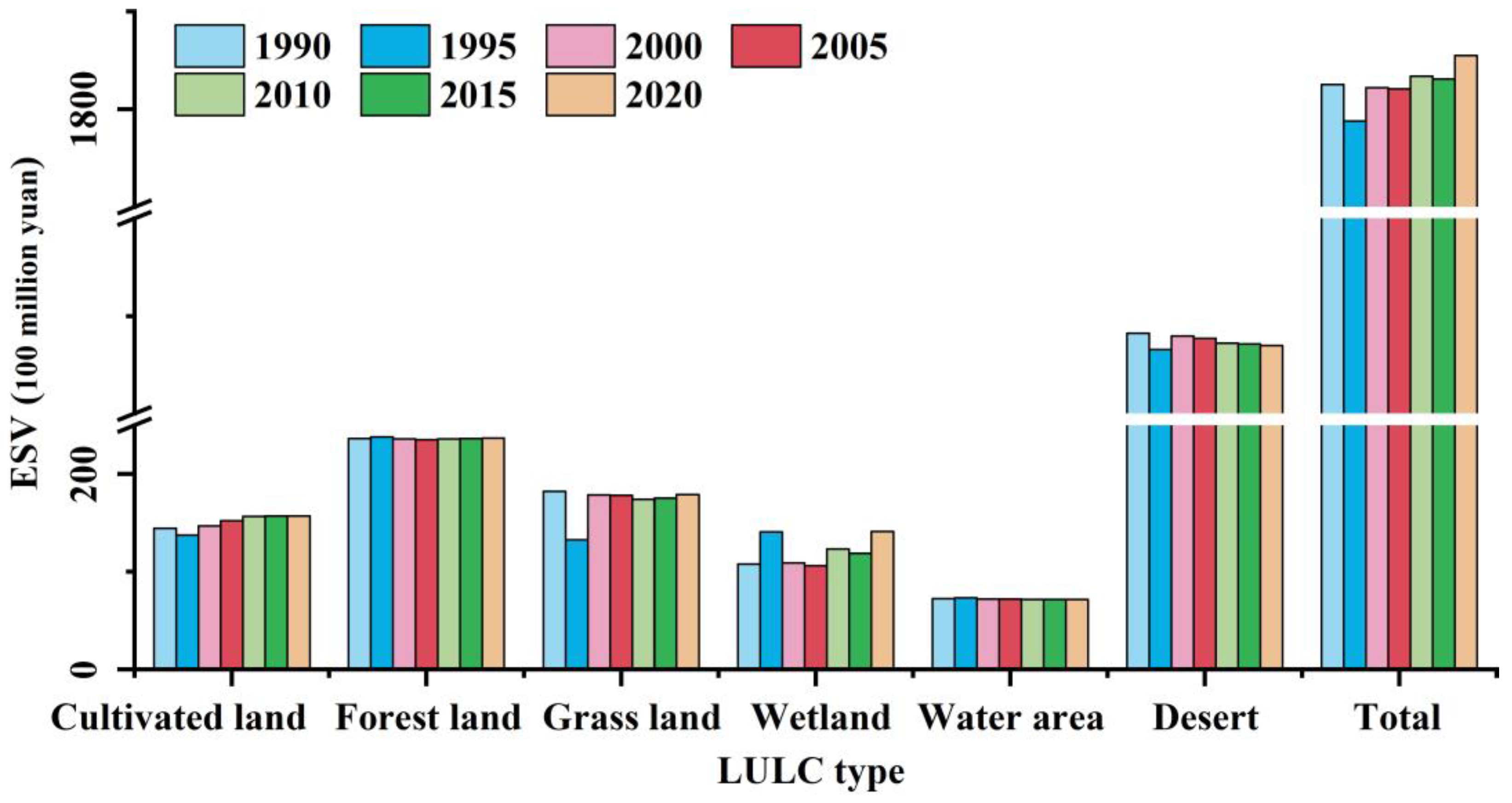
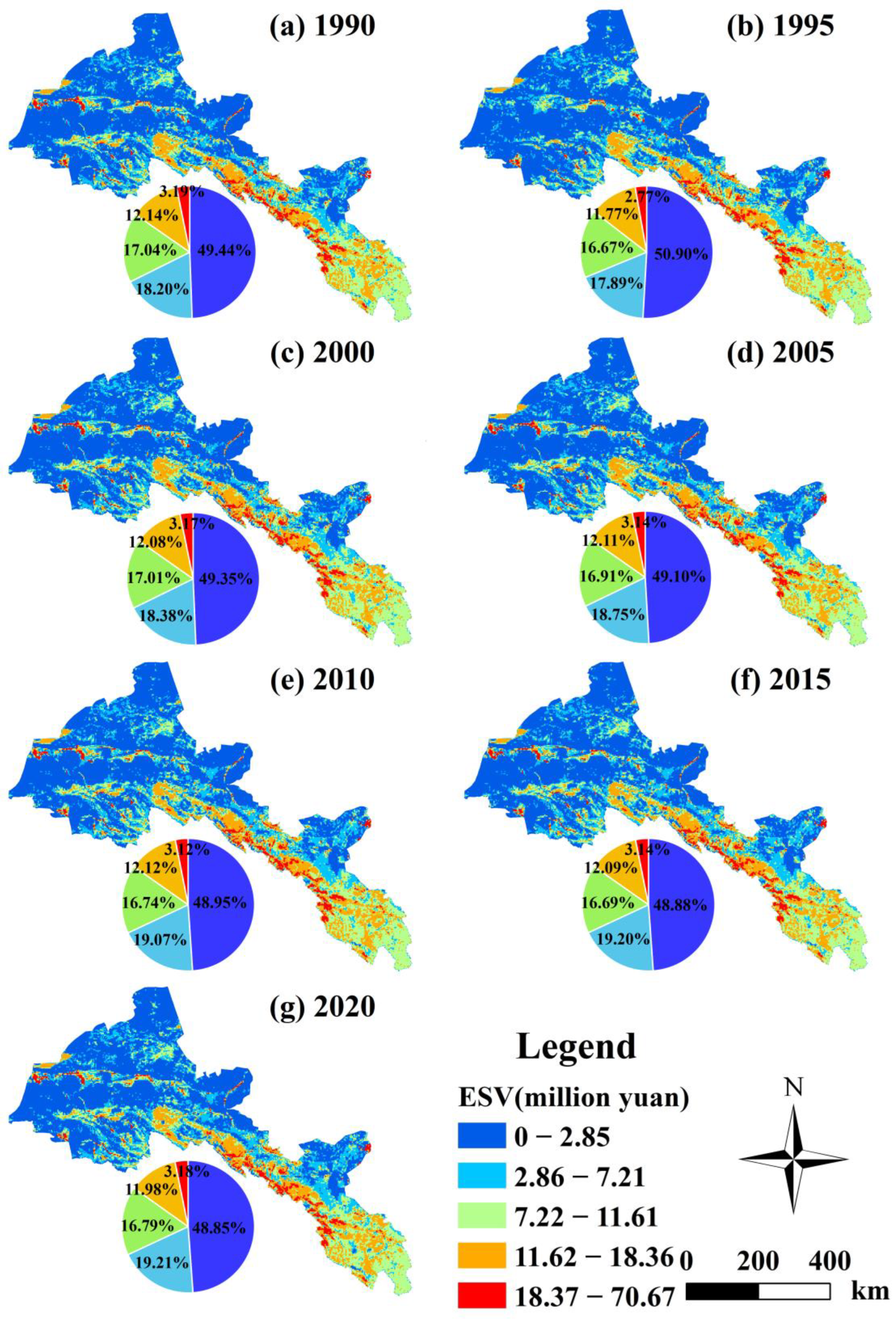
3.2. Spatio-Temporal Variations of ESV

The analysis of ESV variation associated with LULC revealed ESV growth from CNY 182.50 to 185.48 billion between 1990 and 2020 (Figure 5). Distinct variational trends were observed in the ESVs of different LULC types. Cultivated, grassland, forest, and water areas displayed fluctuating upward trends, while wetland and desert ESVs demonstrated fluctuating downward trends. Figure 5 illustrates the proportional contributions of various LULC types to the overall ESV. The proportions of ESV for each LULC type are as follows: grassland (58.85%), forest (12.95%), wetland (9.39%), cultivated land (8.23%), water area (6.63%), and desert (3.95%).
The changes in the value of each type of ecological service vary. Provisioning, regulating, and supporting services all show fluctuating increasing trends, while cultural services exhibit a decreasing trend (Figure 6). Regulating services dominate, representing approximately 64.21% of the total ESV, followed by provisioning (22.74%), support (8.31%), and cultural services (4.74%). Individual ESVs exhibit distinct interannual variation trends (Figure 6). Among them, hydrological regulation, climate regulation, soil conservation, and biodiversity services contribute more than 10% to the total ESV. Hydrological regulation and climate regulation services contribute over 20% to the total ESV. From 2005 to 2020, the single ESV increased significantly in hydrological regulation, water resource supply, and purifying the environment, reflecting remarkable achievements in ecological and environmental protection in HXR.
Over the past 30 years, the total ESV in the HXR has decreased from the southeast to the northwest (Figure 7). This pattern can be attributed to the dominance of deserts with lower ESV in the northwestern part of the HXR, while the southeastern part is characterized by widespread grasslands and forest land with higher ESV. When considering specific urban regions, Jiuquan City boasts the highest ESV, reaching CNY 66.433 billion in 2020, followed by Zhangye City and Wuwei City, while Jiayuguan City has the lowest ESV (Figure 8). The variation in ESV among these cities can be attributed to their total area and LULC types.

3.3. Spatial Autocorrelation of ESV

In addition to examining the spatial and temporal variations of ESV, the degree of spatial aggregation can offer insights into the spatial stability of ESV. A high aggregation degree suggests relative stability and resistance to change, while a low aggregation degree implies greater susceptibility to change. The Moran index is consistently positive in the HXR from 1990 to 2020, indicating non-significant inter-annual variations and reflecting the high spatial clustering of ESV in the region (Table 3). These characteristics are primarily attributed to the considerable spatial aggregation in the LULC structure of the study area. The northwest is primarily occupied by desert, while the southeast is dominated by grasslands, forests, and cultivated land. The areas of high-high value aggregation (HH, hot spot) regions and low-low value aggregation (LL, cold spot) regions undergo varying degrees of transformation, with the hot spot area substantially smaller than the cold spot area (Figure 9). In general, the cities of Zhangye, Wuwei, Lanzhou, and Baiyin host the majority of the hot spot areas in HXR, whereas Jinchang, Jiayuguan, and Jiuquan are home to the majority of the cold spot areas and areas with little reaggregation.

3.4. Contribution of LULC to ESV Change

Frequent transformations of water bodies, cultivated land, grassland, and wetland have resulted in changes in ecological contribution rates (Figure 10). Notably, grassland, wetland, and water bodies have been the major contributors to ESV changes during most periods, with their combined contribution rate exceeding 80%. This indicates that water areas, grasslands, and wetlands are the primary drivers of ESV changes in the HXR over the past 30 years.

3.5. Elasticity Response of the ESV to LULC Changes

The elasticity response of ESV to LULC dynamics reflects the consequences of LULC dynamic transformations on ESV. The overall increase in the ESV sensitivity index from 1990 to 2020 indicates that a 1% change in the comprehensive LULC dynamics degree is associated with changes in ESV of 1.96%, 1.74%, 0.15%, 2.05%, 5.42%, and 9.10%, respectively (Figure 11). This suggests that the influence of LULC dynamics on ESV was significantly enhanced after 2005. The sensitivity index of ESV varies among different service types, with regulating services exhibiting a significantly higher sensitivity index than other service types after 2010. Subsequently, provisioning services demonstrate a relatively lower sensitivity index, followed by supporting services and cultural services, indicating their lower sensitivity to LULC variation (Figure 11b). LULC dynamics have had a substantial impact on hydrological management and water supply since 2005. This is attributed to changes in water and wetland areas, coupled with the stabilization of other LULC patterns through ecological conservation policies. Prior to 2005, services such as food production, material production, and biodiversity were more susceptible to LULC, indicating that during this period, human disturbances predominantly drove changes in LULC, thereby influencing ESV variations in the study area (Figure 11c). In conclusion, the sensitivity of ESV to changes in LULC has been increasing in recent years, especially changes in waters and wetlands that have significantly altered ESV. Based on the high sensitivity of ESV to waters and wetlands, future land management should focus on the protection of waters and wetlands.

4. Discussion

4.1. Driving Factors of LULC Dynamics and Their Impact on the ESV
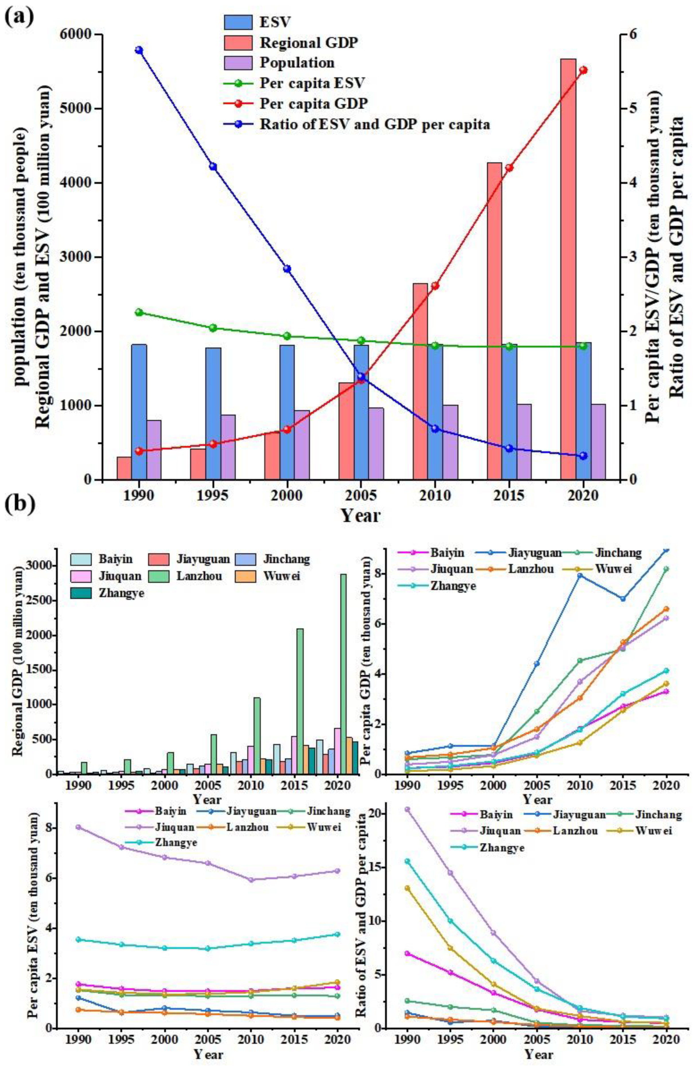
The dynamic interplay between human activities and natural ecology inevitably leads to ecological changes. LULC dynamics are influenced by both social elements (national policies, population, economic development, scientific and technological advancements, etc.) and natural factors (including climate change, natural disasters, and geographical transformations) [56,57]. As LULC changes, the structure and function of ecosystems are inevitably altered to varying degrees [58], which, in turn, affects ESV [59]. Such changes have a more pronounced impact on the ESV [60]. Therefore, given the increasingly pressing ecological and environmental challenges, optimizing LULC structure and formulating or implementing land management policies tailored to local conditions by comparing ESV differences across regions is a promising approach.
The alterations in the HXR’s LULC, which include a decline in desert, grassland, and wetland areas, and a rise in cultivated land, forest, and water areas, are attributed to both natural forcing and human activities acting in combination, as revealed by this study. In the last 50 years, precipitation has increased by 0.14 mm annually [44], mainly in the Qilian Mountains region, leading to an expansion in water area and a gradual conversion of desert to grassland. Human activities such as land reclamation and afforestation are primarily responsible for the spread of forest and agricultural land [38]. Desert and grassland areas are shrinking owing to the joint impacts of natural forcing and human interference. Human intervention has been the dominant driver of LULC changes in the HXR in the recent past, with the establishment of ecological conservation policies, and this effect is not confined to the HXR.
Research has indicated that LULC change is one of the primary driving factors for spatiotemporal variations in ESV [56]. However, during land use planning, the influence of LULC shifts on the natural environment is frequently disregarded. Quantifying and evaluating the effects of LULC variations on ESV can enhance our understanding of land resources and facilitate the formulation of more rational land planning strategies and management policies. In summary, natural forcing and human activities have collectively driven changes in LULC, while the recent implementation of ecological conservation policies has been the dominant factor in the changes of grassland, forest, and cropland. However, it is worth noting that the increase in ESV is primarily contributed by the expansion of water bodies rather than forests, croplands, and grasslands. Therefore, it is imperative to prioritize the conservation of water bodies and wetlands.

4.2. ESV versus GDP

From 1990 to 2020, the HXR experienced a substantial increase in GDP, while the population and ESV exhibited a slower growth rate. The per capita ESV as a percentage of per capita GDP has declined significantly from 5.7914 in 1990 to 0.3268 in 2020 (Figure 12). These findings suggest that despite an overall increase in ESV over the study period, the HXR faces a growing scarcity of ecosystem services due to rapid economic development and limited ecological and environmental resources. This exacerbates the gap between environmental conservation and socioeconomic progress, presenting significant challenges to the continuous promotion of ecological civilization construction [61].
During the period from 1990 to 2020, notable spatial variations were observed in the ESV per capita as a percentage of GDP per capita among cities with different ecosystem structures and levels of economic development (Figure 12). Jiuquan City exhibited the highest ratio, with the largest decline range from 20.43 in 1990 to 1.01 in 2020. This can be attributed to the continuous adjustment and optimization of the industrial structure and rapid economic development. It is also related to the shift in LULC pattern and the relatively slower growth of ESV compared to economic development. Lanzhou had the lowest ratio of per capita ESV to per capita GDP, followed by Jiayuguan, with their ratios decreasing from 1.0898 and 1.4499 in 1990 to 0.0612 and 0.0556 in 2020, respectively. This can be associated with more rapid economic growth and higher levels of development in Lanzhou and Jiayuguan, which resulted in higher population density and limited land area for ecosystem types with higher value coefficients. Consequently, the socioeconomic value gradually caught up with the ESV. Therefore, compared to the socioeconomic value, the ESV exhibited a higher level of scarcity [61]. In summary, the problem of a mismatch between ESV and GDP is widespread in the HXR region, and the rate of economic growth significantly exceeds the rate of increase of ESV. In the future, we should focus on the changes in ESV in Lanzhou, Jiayuguan, and other places to achieve both ecological protection and economic development.

4.3. Comparison ESV with Other Regions

Affected by the interaction of climate and the ecosystem, ESV presents different spatial variations, as indicated by prior investigations [62,63]. Our findings reveal greater ESV in the southern and northeastern regions, while lower in the northwestern regions, which is consistent with previous research. Comparisons with similar areas and ecosystem types reveal that the ESV per unit area in our study (1509 CNY/hm2) is relatively close to values calculated in other studies (1654 CNY/hm2) [61]. Our study also confirms the increasing trend of ESV in the HXR, consistent with research conducted in the south of the Qilian Mountain [64]. Furthermore, we noticed that ecosystem regulation services have the highest value, which is consistent with research conducted in Qilian Mountain National Park [65]. However, our results for forest and grassland ESV differ from those of other studies, particularly in regard to forest ESV per unit area and the long-term variation trend of total grassland ESV [55,66]. These differences can be attributed to variations in methods, indicators, and research periods employed in our study. Additionally, they may also reflect the impact of recent ecological protection governance policies, indirectly indicating the positive influence of anthropogenic activities on ESV improvement.
The estimation of ESV in the HXR may contain uncertainties arising from factors such as research methods, index selection, and parameter setting. For instance, in the reclassification process of LULC types, all urban and rural construction land is grouped into the desert category. This oversimplification overlooks the ESV provided by urban and rural greening initiatives, as well as eco-parks, and fails to account for the negative impact of artificial land surfaces on ESV [67,68]. Consequently, the results may not fully and accurately reflect the ecosystem service status of each city in the HXR. Nonetheless, the findings can serve as a guide for land classification management and environmental preservation in the region.

4.4. Implications of ESV Research for Sustainable Development of Natural-Social Systems

The findings of this study reveal that the three primary land types contributing to ESV changes are water bodies, grasslands, and wetlands. These LULC types are also vulnerable to the impacts of climate change, underscoring the importance of their conservation in the region. Among all LULC types, the conversion between grasslands and deserts emerges as the most frequent transformation in the HXR, significantly influencing ESV variation. Consequently, it is crucial to identify key land types that impact ESV and scrutinize the conversion patterns of these LULC types. For instance, in this study, the conversion from desert to grassland and from cultivated to grassland were identified as the main drivers of grassland expansion. Consequently, interventions can be implemented to increase the area of conversion from desert and cultivated land to grassland, thereby enhancing ESV in the region. This strategic approach has the potential to support the region’s long-term development by providing a theoretical basis for regional environmental protection and land resource management.
Nevertheless, it is crucial to highlight that the HXR grapples with water scarcity [69]. Undertaking large-scale afforestation may not be prudent, as it could escalate water demand and potentially jeopardize the regular water supply to downstream areas [70]. To strike a harmonious balance between ecological enhancement and socio-economic development, future research endeavors should seamlessly integrate ecosystem service value and delve into the optimal trajectory for the sustainable development of both natural and social systems. This objective stands as a pivotal goal in the exploration of ESV.

5. Conclusions

Combined with the unit area equivalent factor method, we conducted an analysis using LULC data and socio-economic data from 1990 to 2020 in the Hexi Corridor Region (HXR). Our study focused on the dynamic changes of LULC types, spatial-temporal variations of Ecosystem Services Value (ESV), and the impact of LULC changes on ESV. Additionally, we developed a sensitivity assessment model to quantify the sensitivity of ESV to LULC changes.
Key findings include the dominance of cultivated land, grassland, and desert as the primary LULC types in the HXR, collectively covering over 95% of the total area. Over the period from 1990 to 2020, the notable characteristics of LULC change involved mutual transformations between grassland and cultivated land, as well as between grassland and desert, occurring at an accelerated rate. During the same period, the ESV in the HXR increased from CNY 182.495 to 185.483 billion, reflecting a total increase of 1.637%. High ESV tends to be concentrated in the southeastern corner, representing the primary geographic area for LULC categories such as grassland, forest, and water bodies. The primary drivers of ESV variation in the HXR over the last 30 years have been water bodies, grassland, and wetland, collectively accounting for 96% of the ecological contribution rate. Notably, the sensitivity of ESV to LULC changes has increased.
Guided by China’s ecological governance regulations, the HXR has experienced gradual improvement in its eco-environmental quality through ecological environment restoration projects. These projects include the conversion of cropland to forests (grasslands) and the management of desertification. However, despite these efforts, the growth of ESV remains relatively slow compared to GDP, leading to a declining ratio of ESV per capita to GDP per capita year by year. This highlights the ongoing conflict between environmental conservation and economic growth. Future research should prioritize the identification of key regions and critical LULC types for ecological protection, aiming to develop a scientifically coordinated development model that balances economic and social development with environmental protection. This approach aims to foster the long-term sustainability of the local economy, society, and natural environment.

Supplementary Materials

The following supporting information can be downloaded at: https://www.mdpi.com/article/10.3390/rs16030563/s1, Table S1: Definition of groups and individual indicators for ecosystem service.

Author Contributions

Conceptualization, B.Z. (Baiting Zhang) and Q.F.; methodology, B.Z. (Baiting Zhang); software, B.Z. (Baiting Zhang); validation, B.Z. (Baiting Zhang), Z.L. (Zongxing Li) and Z.L. (Zhixiang Lu); formal analysis, B.Z. (Baiting Zhang); investigation, W.C.; writing—original draft preparation, B.Z. (Baiting Zhang); writing—review and editing, B.Z. (Baijuan Zhang); funding acquisition, Q.F. and Z.L. (Zhixiang Lu). All authors have read and agreed to the published version of the manuscript.

Funding

This study was supported by the National Natural Science Foundation of China (52179026); the National Key Research and Development Program of China (2022YFF1302600); the “Light of West China” Program of Chinese Academy of Sciences (23JR6KA008) and the major science and technology projects of Gansu Province (23ZDFA018).

Data Availability Statement

The data supporting the findings of this study are available from the corresponding authors under reasonable requirements.

Conflicts of Interest

The authors declare no conflicts of interest.

References

  1. Granstrand, O.; Holgersson, M. Innovation ecosystems: A conceptual review and a new definition. Technovation 2020, 90–91, 102098. [Google Scholar] [CrossRef]
  2. Díaz, S.; Demissew, S.; Carabias, J.; Joly, C.; Lonsdale, M.; Ash, N.; Larigauderie, A.; Adhikari, J.R.; Arico, S.; Báldi, A.; et al. The IPBES Conceptual Framework—Connecting nature and people. Curr. Opin. Environ. Sustain. 2015, 14, 1–16. [Google Scholar] [CrossRef]
  3. Cimatti, M.; Chaplin-Kramer, R.; di Marco, M. The role of high-biodiversity regions in preserving Nature’s Contributions to People. Nat. Sustain. 2023, 6, 1385–1393. [Google Scholar] [CrossRef]
  4. Sannigrahi, S.; Chakraborti, S.; Kumar Joshi, P.; Keesstra, S.; Sen, S.; Paul, S.K.; Kreuter, U.; Sutton, P.C.; Jha, S.; Dang, K.B. Ecosystem service value assessment of a natural reserve region for strengthening protection and conservation. J. Environ. Manag. 2019, 244, 208–227. [Google Scholar] [CrossRef] [PubMed]
  5. Chen, S.; Liu, X.; Yang, L.; Zhu, Z. Variations in Ecosystem Service Value and Its Driving Factors in the Nanjing Metropolitan Area of China. Forests 2023, 14, 113. [Google Scholar] [CrossRef]
  6. Tolessa, T.; Senbeta, F.; Abebe, T. Land use/land cover analysis and ecosystem services valuation in the central highlands of Ethiopia. For. Trees Livelihoods 2017, 26, 111–123. [Google Scholar] [CrossRef]
  7. Ouyang, Z.; Song, C.; Zheng, H.; Polasky, S.; Xiao, Y.; Bateman, I.J.; Liu, J.; Ruckelshaus, M.; Shi, F.; Xiao, Y.; et al. Using gross ecosystem product (GEP) to value nature in decision making. Proc. Natl. Acad. Sci. USA 2020, 117, 14593–14601. [Google Scholar] [CrossRef] [PubMed]
  8. Bateman, I.J.; Harwood, A.R.; Mace, G.M.; Watson, R.T.; Abson, D.J.; Andrews, B.; Binner, A.; Crowe, A.; Day, B.H.; Dugdale, S.; et al. Bringing ecosystem services into economic decision-making: Land use in the United Kingdom. Science 2013, 341, 45–50. [Google Scholar] [CrossRef]
  9. Butler, J.R.A.; Wong, G.Y.; Metcalfe, D.J.; Honzák, M.; Pert, P.L.; Rao, N.; van Grieken, M.E.; Lawson, T.; Bruce, C.; Kroon, F.J.; et al. An analysis of trade-offs between multiple ecosystem services and stakeholders linked to land use and water quality management in the Great Barrier Reef, Australia. Agric. Ecosyst. Environ. 2013, 180, 176–191. [Google Scholar] [CrossRef]
  10. Xu, Y.; Xie, Y.; Wu, X.; Xie, Y.; Zhang, T.; Zou, Z.; Zhang, R.; Zhang, Z. Evaluating temporal-spatial variations of wetland ecosystem service value in China during 1990–2020 from the donor side based on cosmic exergy. J. Clean. Prod. 2023, 414, 137485. [Google Scholar] [CrossRef]
  11. Costanza, R.; de Groot, R.; Braat, L.; Kubiszewski, I.; Fioramonti, L.; Sutton, P.; Farber, S.; Grasso, M. Twenty years of ecosystem services: How far have we come and how far do we still need to go? Ecosyst. Serv. 2017, 28, 1–16. [Google Scholar] [CrossRef]
  12. Zorrilla-Miras, P.; Palomo, I.; Gómez-Baggethun, E.; Martín-López, B.; Lomas, P.L.; Montes, C. Effects of land-use change on wetland ecosystem services: A case study in the Doñana marshes (SW Spain). Landsc. Urban Plan. 2014, 122, 160–174. [Google Scholar] [CrossRef]
  13. Karki, S.; Thandar, A.M.; Uddin, K.; Tun, S.; Aye, W.M.; Aryal, K.; Kandel, P.; Chettri, N. Impact of land use land cover change on ecosystem services: A comparative analysis on observed data and people’s perception in Inle Lake, Myanmar. Environ. Syst. Res. 2018, 7, 25. [Google Scholar] [CrossRef]
  14. Gashaw, T.; Tulu, T.; Argaw, M.; Worqlul, A.W.; Tolessa, T.; Kindu, M. Estimating the impacts of land use/land cover changes on Ecosystem Service Values: The case of the Andassa watershed in the Upper Blue Nile basin of Ethiopia. Ecosyst. Serv. 2018, 31, 219–228. [Google Scholar] [CrossRef]
  15. Li, R.Q.; Dong, M.; Cui, J.Y.; Zhang, L.L.; Cui, Q.G.; He, W.M. Quantification of the impact of land-use changes on ecosystem services: A case study in Pingbian County, China. Environ. Monit. Assess. 2007, 128, 503–510. [Google Scholar] [CrossRef]
  16. Costanza, R.; de Groot, R.; Sutton, P.; van der Ploeg, S.; Anderson, S.J.; Kubiszewski, I.; Farber, S.; Turner, R.K. Changes in the global value of ecosystem services. Glob. Environ. Chang. 2014, 26, 152–158. [Google Scholar] [CrossRef]
  17. Zhang, N.; Dou, S.Q.; Xu, Y.; Jing, J.L.; Zhang, H.B. Temporal spatial changes of ecosystem health in Guangxi in the past 14 years. J. Guilin Univ. Technol. 2021, 41, 370–378. [Google Scholar]
  18. Wang, S.; Zhong, R.; Liu, L.; Zhang, J. Ecological effect of ecological engineering projects on low-temperature forest cover in Great Khingan Mountain, China. Int. J. Environ. Res. Public Health 2021, 18, 10625. [Google Scholar] [CrossRef]
  19. Huang, L.; Qin, X.; Hu, B.; Huang, S.M.; Wei, W.W.; Chen, S.Q. Analysis of Spatial and Temporal Changes in Ecosystem Health and Its Drivers in Southwest Guangxi in the Last 20 Years. J. Guangxi Acad. Sci. 2023, 39, 268–279. [Google Scholar]
  20. Kark, S. Ecotones and Ecological Gradients. In Ecological Systems: Selected Entries from the Encyclopedia of Sustainability Science and Technology; Leemans, R., Ed.; Springer: New York, NY, USA, 2013; pp. 147–160. [Google Scholar]
  21. Huang, Q.; Zhang, F.; Zhang, Q.; Jin, Y.; Lu, X.; Li, X.; Liu, J. Assessing the Effects of Human Activities on Terrestrial Net Primary Productivity of Grasslands in Typical Ecologically Fragile Areas. Biology 2023, 12, 38. [Google Scholar] [CrossRef] [PubMed]
  22. Li, C.; Fu, B.; Wang, S.; Stringer, L.C.; Wang, Y.; Li, Z.; Liu, Y.; Zhou, W. Drivers and impacts of changes in China’s drylands. Nat. Rev. Earth Environ. 2021, 2, 858–873. [Google Scholar] [CrossRef]
  23. Zhang, Z.; Huisingh, D. Combating desertification in China: Monitoring, control, management and revegetation. J. Clean. Prod. 2018, 182, 765–775. [Google Scholar] [CrossRef]
  24. Xie, Y.; Zhang, L.; Gong, X.; Liu, J.; Liao, X.; Dong, Y. Empirical study of the coupling relationship between biodiversity and environmental geology under different ecological status: Evidence from five typical areas in Guizhou, China. Environ. Sci. Pollut. Res. 2022, 29, 51398–51410. [Google Scholar] [CrossRef] [PubMed]
  25. Zhao, B.; Zhao, Y.Q. Investigation and analysis of the Xiangning landslide in Shanxi Province, China. Nat. Hazards 2020, 103, 3837–3845. [Google Scholar] [CrossRef]
  26. Tan, W.; Li, X. Guidance of the coordination theory of man-land relationship to land exploitation and utilization. In Proceedings of the 2017 4th International Conference on Industrial Economics System and Industrial Security Engineering (IEIS), Kyoto, Japan, 24–27 July 2017. [Google Scholar] [CrossRef]
  27. Xie, W.; Huang, Q.; He, C.; Zhao, X. Projecting the impacts of urban expansion on simultaneous losses of ecosystem services: A case study in Beijing, China. Ecol. Indic. 2018, 84, 183–193. [Google Scholar] [CrossRef]
  28. Jiang, C.; Nath, R.; Labzovskii, L.; Wang, D. Integrating ecosystem services into effectiveness assessment of ecological restoration program in northern China’s arid areas: Insights from the Beijing-Tianjin Sandstorm Source Region. Land Use Policy 2018, 75, 201–214. [Google Scholar] [CrossRef]
  29. Wang, Z.J.; Liu, S.J.; Li, J.H.; Pan, C.; Wu, J.L.; Ran, J.; Su, Y. Remarkable improvement of ecosystem service values promoted by land use/land cover changes on the Yungui Plateau of China during 2001–2020. Ecol. Indic. 2022, 142, 109303. [Google Scholar] [CrossRef]
  30. Wang, S.D.; Zhang, H.B.; Wang, X.C. Analysis on the dynamic changes in a regional ecosystem and evaluation of its service values based on remote sensing. Int. Arch. Photogramm. Remote Sens. Spat. Inf. Sci.-ISPRS Arch. 2015, 47, 169–174. [Google Scholar] [CrossRef]
  31. Pan, N.; Guan, Q.; Wang, Q.; Sun, Y.; Li, H.; Ma, Y. Spatial Differentiation and Driving Mechanisms in Ecosystem Service Value of Arid Region: A case study in the middle and lower reaches of Shule River Basin, NW China. J. Clean. Prod. 2021, 319, 128718. [Google Scholar] [CrossRef]
  32. Cheng, W.; Shen, B.; Xin, X.; Gu, Q.; Guo, T. Spatiotemporal Variations of Grassland Ecosystem Service Value and Its Influencing Factors in Inner Mongolia, China. Agronomy 2022, 12, 2090. [Google Scholar] [CrossRef]
  33. Zhang, S.; Chen, C.; Yang, Y.; Huang, C.; Wang, M.; Tan, W. Coordination of economic development and ecological conservation during spatiotemporal evolution of land use/cover in eco-fragile areas. Catena 2023, 226, 107097. [Google Scholar] [CrossRef]
  34. Li, X.; Yang, L.; Tian, W.; Xu, X.F.; He, C.S. Land use and land cover change in agro-pastoral ecotone in Northern China: A review. Chin. J. Appl. Ecol. 2018, 29, 3487–3495. [Google Scholar]
  35. Han, L.; Zhang, Z.; Zhang, Q.; Wan, X. Desertification assessments in the Hexi corridor of northern China’s Gansu Province by remote sensing. Nat. Hazards 2015, 75, 2715–2731. [Google Scholar] [CrossRef]
  36. Li, T.; Zhang, Q.; Singh, V.P.; Zhao, J.; Song, J.; Sun, S.; Wang, G.; Shen, Z.; Wu, W. Identification of Degradation Areas of Ecological Environment and Degradation Intensity Assessment in the Yellow River Basin. Front. Earth Sci. 2022, 10, 922013. [Google Scholar] [CrossRef]
  37. Du, X.; Qin, Y.; Huang, C. Status and Prospect of Ecological Environment in the Belt and Road Initiative Regions. Int. J. Environ. Res. Public Health 2022, 19, 17091. [Google Scholar] [CrossRef] [PubMed]
  38. Li, K.; Zhang, B. Spatial-temporal Change Characteristics and Driving Factors of Land Use in Hexi corridor. Geomat. Spat. Inf. Technol. 2023, 46, 75–81. [Google Scholar]
  39. Pan, N.; Du, Q.; Guan, Q.; Tan, Z.; Sun, Y.; Wang, Q. Ecological security assessment and pattern construction in arid and semi-arid areas: A case study of the Hexi Region, NW China. Ecol. Indic. 2022, 138, 108797. [Google Scholar] [CrossRef]
  40. Wei, W.; Liu, C.; Liu, C.; Xie, B.; Zhou, J.; Nan, S. Spatio-temporal analysis of ecological vulnerability in arid region: A case study of hexi corridor, northwest China. Hum. Ecol. Risk Assess. Int. J. 2022, 28, 564–593. [Google Scholar] [CrossRef]
  41. Xue, J.; Li, Z.X.; Chen, X.J.; Zhou, H.L.; Gui, J. Spatial and temporal variation of ecosystem service functions in the Hexi region from 2000 to 2020 and its influence factors analysis. Environ. Ecol. 2023, 5, 1–12. [Google Scholar]
  42. Wang, G.; Cheng, G.; Shen, Y. Features of eco-environmental changes in Hexi Corridor Region in the last 50 years and comprehensive control strategies. J. Nat. Resour. 2002, 17, 78–86. [Google Scholar]
  43. Cheng, W.; Feng, Q.; Xi, H.; Yin, X.; Sindikubwabo, C.; Habiyakare, T.; Chen, Y.; Zhao, X. Spatiotemporal variability and controlling factors of groundwater depletion in endorheic basins of Northwest China. J. Environ. Manag. 2023, 344, 118468. [Google Scholar] [CrossRef]
  44. Feng, Q.; Li, Z.; Liu, W.; Li, J.; Guo, X.; Wang, T. Relationship between large scale atmospheric circulation, temperature and precipitation in the Extensive HXR, China, 1960–2011. Quat. Int. 2016, 392, 187–196. [Google Scholar] [CrossRef]
  45. Fan, D.; Ni, L.; Jiang, X.; Fang, S.; Wu, H.; Zhang, X. Spatiotemporal Analysis of Vegetation Changes along the Belt and Road Initiative Region from 1982 to 2015. IEEE Access 2020, 8, 122579–122588. [Google Scholar] [CrossRef]
  46. Han, X.; Yu, J.; Shi, L.; Zhao, X.; Wang, J. Spatiotemporal evolution of ecosystem service values in an area dominated by vegetation restoration: Quantification and mechanisms. Ecol. Indic. 2021, 131, 108191. [Google Scholar] [CrossRef]
  47. Xie, G.; Zhang, C.; Zhang, L.; Chen, W.H.; Li, S.M. Improvement of the evaluation method for ecosystem service value based on per unit area. J. Nat. Resour. 2015, 30, 1243–1254. [Google Scholar]
  48. Zheng, D.F.; Hao, S.; Lv, L.T.; Xu, W.J.; Wang, Y.Y.; Wang, H. Spatial-temporal change and trade-off/synergy relationships among multiple ecosystem services in Three-River-Source National Park. Geogr. Res. 2020, 39, 64–78. [Google Scholar]
  49. Huang, B.; Huang, J.; Pontius, R.G.; Tu, Z. Comparison of Intensity Analysis and the land use dynamic degrees to measure land changes outside versus inside the coastal zone of Longhai, China. Ecol. Indic. 2018, 89, 336–347. [Google Scholar] [CrossRef]
  50. Qiu, H.; Hu, B.; Zhang, Z. Study on ecosystem service value of Guangxi in the past 20 years based on land use change. J. Environ. Eng. Technol. 2022, 12, 1455–1465. [Google Scholar]
  51. Liu, Z.; Wang, S.; Fang, C. Spatiotemporal evolution and influencing mechanism of ecosystem service value in the Guangdong-Hong Kong-Macao Greater Bay Area. J. Geogr. Sci. 2021, 33, 1226–1244. [Google Scholar] [CrossRef]
  52. Li, Y.; Liu, W.; Feng, Q.; Zhu, M.; Yang, L.; Zhang, J.; Yin, X. The role of land use change in affecting ecosystem services and the ecological security pattern of the Hexi Regions, Northwest China. Sci. Total Environ. 2023, 855, 158940. [Google Scholar] [CrossRef]
  53. Mengist, W.; Soromessa, T.; Feyisa, G.L. Estimating the total ecosystem services value of Eastern Afromontane Biodiversity Hotspots in response to landscape dynamics. Environ. Sustain. Indic. 2022, 14, 100178. [Google Scholar] [CrossRef]
  54. Chen, W.; Liu, Z.; Li, J.; Ran, D.; Zeng, J. Mapping the spatial relationship between ecosystem services and urbanization in the middle reaches of the Yangtze River Urban Agglomerations. Acta Ecol. Sin. 2020, 40, 5137–5150. [Google Scholar] [CrossRef]
  55. Zhang, X.B.; Luo, J.; Shi, P.J.; Zhou, L. Spatial-temporal evolution pattern and terrain gradient differentiation of ecosystem service value in Zhangye, Northwest China at the grid scale. Chin. J. Appl. Ecol. 2020, 31, 543–553. [Google Scholar]
  56. Lambin, E.F.; Meyfroidt, P. Global land use change, economic globalization, and the looming land scarcity. Proc. Natl. Acad. Sci. USA 2011, 108, 3465–3472. [Google Scholar] [CrossRef]
  57. Qiu, L.; Pan, Y.; Zhu, J.; Amable, G.S.; Xu, B. Integrated analysis of urbanization-triggered land use change trajectory and implications for ecological land management: A case study in Fuyang, China. Sci. Total Environ. 2019, 660, 209–217. [Google Scholar] [CrossRef]
  58. Wu, C.; Chen, B.; Huang, X.; Dennis Wei, Y.H. Effect of land-use change and optimization on the ecosystem service values of Jiangsu province, China. Ecol. Indic. 2020, 117, 106507. [Google Scholar] [CrossRef]
  59. Polasky, S.; Nelson, E.; Pennington, D.; Johnson, K.A. The impact of land-use change on ecosystem services, biodiversity and returns to landowners: A case study in the state of Minnesota. Environ. Resour. Econ. 2011, 48, 219–242. [Google Scholar] [CrossRef]
  60. Shiferaw, H.; Bewket, W.; Alamirew, T.; Zeleke, G.; Teketay, D.; Bekele, K.; Schaffner, U.; Eckert, S. Implications of land use/land cover dynamics and Prosopis invasion on ecosystem service values in Afar Region, Ethiopia. Sci. Total Environ. 2019, 675, 354–366. [Google Scholar] [CrossRef]
  61. Xu, Q.; Wang, Y.; Yang, Y. Spatio-temporal evaluation of ecosystem service value in Gansu Province based on optimization model. J. Desert Res. 2023, 43, 53–64. [Google Scholar]
  62. Xie, G.; Zhang, C.; Zhen, L.; Zhang, L. Dynamic changes in the value of China’s ecosystem services. Ecosyst. Serv. 2017, 26, 146–154. [Google Scholar] [CrossRef]
  63. Zeng, Q.; Ye, X.; Cao, Y.; Chuai, X.; Xu, H. Impact of expanded built-up land on ecosystem service value by considering regional interactions. Ecol. Indic. 2023, 153, 110397. [Google Scholar] [CrossRef]
  64. Qian, D.; Cao, G.; Du, Y.; Li, Q.; Guo, X.W. Spatio-temporal dynamics of ecosystem service value in the southern slope of Qilian Mountain from 2000 to 2015. Acta Ecol. Sin. 2020, 40, 1392–1404. [Google Scholar]
  65. Fan, Z.; Li, N.; Li, W. Evaluation of the ecosystem service value of the Qilian Mountain National Park in Gansu Province. Contemp. Econ. 2021, 12, 70–77. [Google Scholar]
  66. Shao, M.; Ma, L.; Wang, X.; Che, X.H.; Wang, F.; Lu, J.F.; Luo, W.Y. The valuation of ecosystem service value of desertification grassland from 2004 to 2014 in Hexi Corridor, China. J. Desert Res. 2022, 42, 63–73. [Google Scholar]
  67. Liu, H.; Wu, J.; Chen, X. Study on spatial-temporal change andtrade-off/synergy relationships of ecosystem services in the Danjiangkou water source area. Acta Ecol. Sin. 2018, 38, 4609–4624. [Google Scholar]
  68. Zhao, Y.F.; Han, Z.B.; Xu, Y.Q. Impact of Land Use/Cover Change on Ecosystem Service Value in Guangxi. Sustainability 2022, 14, 10867. [Google Scholar] [CrossRef]
  69. Wang, S.; Liu, H.; Yu, Y.; Zhao, W.; Yang, Q.; Liu, J. Evaluation of groundwater sustainability in the arid Hexi Corridor of Northwestern China, using GRACE, GLDAS and measured groundwater data products. Sci. Total Environ. 2020, 705, 135829. [Google Scholar] [CrossRef]
  70. Lim, C.H.; Song, C.; Choi, Y.; Jeon, S.W.; Lee, W.K. Decoupling of forest water supply and agricultural water demand attributable to deforestation in North Korea. J. Environ. Manag. 2019, 248, 109256. [Google Scholar] [CrossRef]
Figure 1. The location and basic information of study area. (a) is the LULC spatial distribution of HXR, and (b) is the remote sensing image of HXR. The red line in subplot (b) is study boundary.
Remotesensing 16 00563 g001
Figure 2. Spatio-temporal variation of each LULC category area from 1990 to 2020. The pie chart represents the proportion of the area of each LULC area to the total area from 1990 to 2020.
Remotesensing 16 00563 g002
Figure 3. Comprehensive and single dynamic degree changes of LULC in HXR during 1990–2020. (a) is the comprehensive dynamic degree of LULC; (b) is the single dynamic degree of each LULC-type.
Remotesensing 16 00563 g003
Figure 4. Transformation of the LULC area of six study periods in HXR.
Remotesensing 16 00563 g004
Figure 5. Temporal variation of ESV for the total and each LULC type in HXR during 1990–2020.
Remotesensing 16 00563 g005
Figure 6. Temporal variation of ESV for 4 service groups and 11 individual service indicators in HXR during 1990–2020. (ad) represents time changes in the value of provisioning services, regulating services, supporting services and cultural services, respectively. (eo) represents time changes in the value of food production, material production, water resources supply, gas regulation, climate regulation, purify environment, hydrological regulation, soil conservation, maintain nutrient cycle, biodiversity and aesthetic landscape, respectively.
Remotesensing 16 00563 g006
Figure 7. Geographical distribution of total ESV on a grid scale during 1990–2020. The pie chart represents the proportion of the area of ESV within each interval relative to the total area.
Remotesensing 16 00563 g007
Figure 8. ESV variation for each administrative region and the proportion of ESV for each administrative region to the total ESV. subplots (ag) represent the temporal variation of ESV in the municipalities of Baiyin, Jiayuguan, Jinchang, Jiuquan, Lanzhou, Wuwei, and Zhangye, respectively.
Remotesensing 16 00563 g008
Figure 9. Hotspot analysis of ESV in HXR during 1990–2020.
Remotesensing 16 00563 g009
Figure 10. Change rate in ESV for each LULC and its contribution to total ESV change in HXR.
Remotesensing 16 00563 g010
Figure 11. Change rate of ESV and its sensitivity to LULC changes. (a) is the total ESV change rate and its sensitivity to LULC variations, (b) is the dynamic rate of each ESV type and its sensitivity to LULC variations, and (c) is the dynamic rate of individual ESV and its sensitivity to LULC variations.
Remotesensing 16 00563 g011
Figure 12. The temporal dynamic of GDP, ESV, population, per capita ESV/GDP, ratio of ESV and GDP per capita from 1990 to 2020. (a) is the change in these indicators over time across the entire HXR; (b) is the change in these indicators for each municipality.
Remotesensing 16 00563 g012
Table 1. The adjusted standard equivalent factor of ESV per unit area.
Ecosystem Service TypeEcosystem Type
GroupsIndicatorsCultivated LandForest LandGrasslandWetlandWater AreaDesert
Provisioning servicesFood production0.85000.23000.19000.51000.29000.0001
Material production0.40000.53000.27000.50000.08000.0001
Water resources supply0.02000.27000.15002.59004.39000.0001
Regulating servicesGas regulation0.67001.74000.97001.90000.39000.0300
Climate regulation0.36005.21002.57003.60001.18000.0100
Purify environment0.10001.53000.85003.60002.12000.1200
Hydrological regulation0.27003.39001.880024.230041.78000.0500
Supporting servicesSoil conservation1.03002.12001.18002.31000.34000.0300
Maintain nutrient cycle0.12000.16000.09000.18000.03000.0001
Biodiversity0.13001.93001.07007.87000.94000.0300
Cultural servicesAesthetic landscape0.06000.85000.48004.73000.75000.0100
Total4.009917.96009.700052.020052.29000.2804
Table 2. The individual ESV of different ecosystem types per unit area in the HXR.
Ecosystem Service TypeEcosystem Type
GroupsIndicatorsCultivated LandForest LandGrasslandWetlandWater AreaDesert
Provisioning servicesFood production1.2830.34720.28680.76980.43770.0002
Material production0.60380.80000.40760.75470.12080.0002
Water resources supply0.03020.40760.22643.90956.62650.0002
Regulating servicesGas regulation1.01132.62651.46422.86800.58870.0453
Climate regulation0.54347.86433.87935.43411.78120.0151
Purify environment0.15092.30951.28305.43413.20010.1811
Hydrological regulation0.40765.11712.837836.574263.06520.0755
Supporting servicesSoil conservation1.55473.20011.78123.48690.51320.0453
Maintain nutrient cycle0.18110.24150.13590.27170.04530.0002
Biodiversity0.19622.91331.615111.87951.41890.0453
Cultural servicesAesthetic landscape0.09061.28300.72457.13971.13210.0151
Total6.052927.109914.641878.522178.92970.4233
Note: unit: 105 CNY·km−2·a−1.
Table 3. Moran’s index and Z-scores of the spatial distribution of ESV in different periods in HXR.
1990199520002005201020152020
Moran’s Index0.75020.77420.75210.75280.75140.75200.7511
z-score169.95175.38170.37170.54170.19170.35170.11
Note: The Moran’s Index for each year has passed a significance test with a p-value < 0.01.
Disclaimer/Publisher’s Note: The statements, opinions and data contained in all publications are solely those of the individual author(s) and contributor(s) and not of MDPI and/or the editor(s). MDPI and/or the editor(s) disclaim responsibility for any injury to people or property resulting from any ideas, methods, instructions or products referred to in the content.

