Multi-Frequency Polarimetric SAR Classification Based on Riemannian Manifold and Simultaneous Sparse Representation

Abstract

Normally, polarimetric SAR classification is a high-dimensional nonlinear mapping problem. In the realm of pattern recognition, sparse representation is a very efficacious and powerful approach. As classical descriptors of polarimetric SAR, covariance and coherency matrices are Hermitian semidefinite and form a Riemannian manifold. Conventional Euclidean metrics are not suitable for a Riemannian manifold, and hence, normal sparse representation classification cannot be applied to polarimetric SAR directly. This paper proposes a new land cover classification approach for polarimetric SAR. There are two principal novelties in this paper. First, a Stein kernel on a Riemannian manifold instead of Euclidean metrics, combined with sparse representation, is employed for polarimetric SAR land cover classification. This approach is named Stein-sparse representation-based classification (SRC). Second, using simultaneous sparse representation and reasonable assumptions of the correlation of representation among different frequency bands, Stein-SRC is generalized to simultaneous Stein-SRC for multi-frequency polarimetric SAR classification. These classifiers are assessed using polarimetric SAR images from the Airborne Synthetic Aperture Radar (AIRSAR) sensor of the Jet Propulsion Laboratory (JPL) and the Electromagnetics Institute Synthetic Aperture Radar (EMISAR) sensor of the Technical University of Denmark (DTU). Experiments on single-band and multi-band data both show that these approaches acquire more accurate classification results in comparison to many conventional and advanced classifiers.

1. Introduction

During recent decades, there have been a number of applications of polarimetric SAR (Synthetic Aperture Radar) for land cover classification in the field of remote sensing. Traditionally, classification approaches based on statistical distribution assumptions are used. Kong [1] and Lim [2] proposed a Bayes classifier based on complex Gaussian distribution for single-look polarimetric SAR, which uses the fully-polarimetric information first. Lee [3] refined their method and developed an optimal classifier for multi-look polarimetric SAR data based on the complex Wishart distribution, named the Wishart classifier. However, only in homogeneous land cover cases does the Wishart distribution assumption hold; that is, it does not hold well in heterogeneous land cover cases, like high-resolution images [4], leading to the weak performance of the classification based on this assumption. To solve this problem, many complicated distribution models for heterogeneous land cover are proposed, such as the work by Vasile [5] and the KummerU model by Bombrun [6]. These classification approaches based on distribution assumptions often have common disadvantages of complex parameter estimation and limited model suitability. As the number of the parameters increases, it is difficult to estimate these parameters accurately with a small group of training samples. Meanwhile, it is difficult to adjust a distribution model to all of the complex land covers. The mixed Gaussian model by Gao [7] is a well-designed novel heterogeneous model, but still faces the problem of complex parameter estimations, especially when training samples are inadequate.

Other choices are classification approaches based on regions, which exploit spatial correlations between neighboring pixels [8]. Images are first segmented into small regions containing pixels with similar properties, and then, the class label to a region is determined jointly as a whole. For instance, Wu [9] projected such a method, which employs the Markov random field (MRF). Despite more classification accuracy due to additional information of spatial correlations, it also induces extra complication in modeling and computation. Therefore, pixel-based classification approaches attaining comparable accuracy are still preferable, and hence, this paper still discusses pixel-based classification schemes.

Alternatively, this paper explores another classification approach without complicated distribution assumptions and neighborhood modeling. Theoretically, covariance matrices and coherency matrices of polarimetric SAR are Hermitian symmetric positive semi-definite, and experiments show that almost all of the polarimetric SAR data follow that rule. Hermitian symmetric positive semi-definite matrices can be regarded as tensors, which form a Riemannian manifold. Hence, some metrics in Riemannian manifolds can be introduced to measure the similarities and distances between polarimetric SAR data in feature space, which are expected to induce new classification methods. The new methods do not rely on certain distribution assumptions and are flexible and suitable for more polarimetric SAR data in different land cover cases. A few researchers have utilized Riemannian manifolds for polarimetric SAR segmentation [10] and classification [11]. A common and effective metric on Riemannian manifolds is geodesic distance, but it is difficult to calculate [12], which involves lots of matrix eigenvalue decompositions. To reduce the computing complexity, the log-Euclidean metric [13] and Stein divergence [14] are employed. The former also involves eigenvalue decomposition, while the latter only contains the calculation of matrix determinants, which is more desirable.

In the realm of pattern recognition, sparse representation is a very efficacious and powerful approach, which has been used in diverse application from image denoising to target classification. According to these methods, a target signal is approximated using a sparse linear combination of elementary signals called “atoms” from a large candidate set named “dictionary”. For example, Wright proposed SRC (sparse representation-based classification) [15] for classification and recognition of objects, such as faces. In the field of polarimetric SAR, Xu [16] introduced sparse representation to filtering and reducing speckles and achieved good performance. Zhang [17] used sparse methods to represent polarimetric SAR features, such as entropy, and applied them to land cover classification. However, these features do not form a Euclidean space and may be not compatible with SRC on a Euclidean space. Harandi [18] tackles the problem of sparse coding and dictionary learning in the space of a Riemannian manifold. With the help of the aforementioned Stein divergence [14], Harandi [18] performs sparse coding by embedding Riemannian manifolds into kernel Hilbert spaces. This engenders an unconstrained minimization least-squares with a penalty term of the one-norm of the parameter vector. This is a convex and kernel version of Lasso problem [25], which can be solved using quadratic programming or more general convex optimization approaches, as well as by specific algorithms, such as the least angle regression algorithm. The l1-norm regularized formulation is useful, owing to its tendency to choose solutions with fewer nonzero parameter values. Additionally, for this reason, the Lasso and its variants are fundamental to the field of compressed sensing. Based on SRC [15] and Stein kernel sparse representation on Riemannian manifolds [18], this paper propose a polarimetric SAR land cover classification approach.

There are several frequency bands for SAR radar, including the P band, L band, C band, and so on. Land cover exhibits different scattering properties corresponding to different bands. In the field of polarimetric SAR classification, multi-band information merging can markedly enhance the accuracy of classification. This is similar to the situations in sensor networks, in which the same physical information is transmitted through different channels or detected by different sensors. Simultaneous sparse representation [19,20] is often exploited to describe such phenomena. Enlightened by these methods, this paper proposes a pixel-level merging approach. Based on the reasonable assumption of sparse representative correlation among different bands, we merge data from several bands naturally through simultaneous sparse representation. Therefore, our approach can be generalized successfully to multi-band polarimetric SAR classification.

Two innovative points are involved in our research. One, SRC based on a Stein kernel on a Riemannian manifold, is firstly introduced into polarimetric SAR. Wang [10] combines a Riemannian manifold with mean-shift in segmentation applications, and Song [11] combines a Riemannian manifold with k-means in classification. Both involve the mean calculation of tensor space, which involves iterations and is time consuming. Additionally, the former only discusses the geodesic distance and log-Euclidean distance, which is also complicated. In addition, different from Zhang [17], which also employs SRC, our approach classifies polarimetric SAR data directly rather than artificially extracting several features first, and this circumvents the loss of information. Based on some reasonable assumptions and necessary transformations, this paper first successfully applies simultaneous SRC to multi-frequency polarimetric SAR land cover classification.

The remainder of this paper is organized as follows. Some background research is summarized in Section 2, including basic properties and classifiers of polarimetric SAR data, the introduction of the Riemannian manifold, the Stein kernel and the SRC approach. In Section 3, the Stein-SRC approach, a classification scheme based on sparse representation, is presented in detail and generalized to a multi-band application with simultaneous sparse representation. Experiment results are given in Section 4 with discussions. Finally, the research is concluded in Section 5.

2. Background Research

2.1. Basic Properties and Wishart Classifier of Polarimetric SAR

Fully-polarimetric SAR data usually contain the amplitude and phase of backscattering signals in four combinations of the linear receive and transmit polarizations: HH, HV, VH and VV. Each resolution pixel is described by a 2 × 2 complex scattering matrix S, or the Sinclair matrix, as shown in Equation (1).

$$\mathbf{S}=\left[\begin{array}{cc}\begin{array}{l}{S}_{HH}\\ S_{VH}\end{array}& \begin{array}{l}{S}_{HV}\\ S_{VV}\end{array}\end{array}\right]$$

(1)

In the case of monostatic backscattering in a reciprocal medium, S_HV = S_VH. The lexicographic scattering vector ${\overrightarrow{k}}_l$ and Pauli scattering vector ${\overrightarrow{k}}_p$ are often used to describe the scattering properties of the land cover as follows.

$$\begin{array}{c}{\overrightarrow{k}}_l={\left[S_{HH}\sqrt{2}{S}_{HV}{S}_{VV}\right]}^T\\ {\overrightarrow{k}}_p={\left[\frac{S_{HH}+S_{VV}{S}_{HH}-S_{VV}2S_{HV}}{\sqrt{2}}\right]}^T\end{array}$$

(2)

where superscript T denotes the transpose of the vector. Moreover, for the purpose of speckle reduction, scattering vectors of adjacent resolution units are incoherently spatial averaged or multi-look processed at the expense of the loss of spatial resolution. Therefore, for a complex target, the scattering characteristics should be described by statistic covariance matrix C or coherency matrix T, which can be generated from the outer product of ${\overrightarrow{k}}_l$ and ${\overrightarrow{k}}_p$,

$$\begin{array}{c}\mathbf{C}=\frac{1}{n}{\displaystyle \sum _{i=1}^N{\overrightarrow{k}}_l{\overrightarrow{k}}_l^H}\\ \mathbf{T}=\frac{1}{n}{\displaystyle \sum _{i=1}^N{\overrightarrow{k}}_p{\overrightarrow{k}}_p^H}\end{array}$$

(3)

where H denotes the conjugate transpose of a matrix and n is defined as the number of looks. From the equation above, we can confirm that covariance matrix C and coherency matrix T are both Hermitian positive semidefinite. For ∀x:

$$\begin{array}{c}{\mathbf{x}}^H\mathbf{Cx}={\displaystyle \sum {}_{i=1}^L{\left({\overrightarrow{k}}_l^H\mathbf{x}\right)}^H{\overrightarrow{k}}_l^H\mathbf{x}\ge 0}\\ {\mathbf{x}}^H\mathbf{Tx}={\displaystyle \sum {}_{i=1}^L{\left({\overrightarrow{k}}_p^H\mathbf{x}\right)}^H{\overrightarrow{k}}_p^H\mathbf{x}\ge 0}\end{array}$$

(4)

The coherency covariance matrix and matrix contain the same information and can be transformed by some relative transformations; hence, we will use coherency matrix T as a representative for convenience.

Many statistical models have been proposed for multi-look polarimetric SAR data, among which the Wishart model is fundamental. For homogeneous regions, as demonstrated by Goodman [21], if the scattering vectors ${\overrightarrow{k}}_p$ are independent, then T has a complex Wishart distribution, the probability density function of which is:

$$p(\mathbf{T}|\mathbf{Z})=\frac{n^{nd}{\left|\mathbf{T}\right|}^{n-d}\exp \{-nTr({\mathbf{Z}}^{-1}\mathbf{T})\}}{R(n,d){\left|\mathbf{Z}\right|}^n}$$

(5)

where Z denotes the centroid of the distribution, Tr denotes the trace of a matrix and R(n, d) can be calculated as:

$$R(n,d)={\pi }^{\frac{d(d-1)}{2}}\Gamma (n)\cdots \Gamma (n-d+1)$$

(6)

where Γ (·) represents the gamma function and the parameter d in Equations (5) and (6) is the dimension of the scattering vector. For a fully-polarimetric SAR under the reciprocity assumption, d = 3. Based on the Wishart model above, Lee [3] has proposed an optimal Bayes classifier for multi-look polarimetric SAR data. A distance measure is also derived by Lee [3], representing the distance between a test sample with coherency matrix T and a class ω_m, i.e.,

$$d_W(\mathbf{T},{\omega }_{\mathbf{m}})=\text{log}\left|{\mathbf{Z}}_{\mathbf{m}}\right|+Tr({\mathbf{Z}}_{\mathbf{m}}^{-1}\mathbf{T})$$

(7)

which is minimized among all classes when performing classification for T. Zm represents the ensemble mean of coherency matrices corresponding to the m-th class. For multi-frequency SAR, the merging Wishart classifier assigns the pixel to the class that minimizes the sum of the Wishart distance to the class center of L, P and C bands data. The Wishart classifier is a milestone for polarimetric SAR land cover classification for its effectiveness and low computing complexity.

2.2. Introduction of the Riemannian Manifold and Stein Kernel

The elements in Hermitian positive semidefinite matrices, like C and T in Equations (3) and (4), cannot be endowed any arbitrary values. There exists some intrinsic association between these elements. Mathematically, these matrices form a Riemannian manifold. On a Riemannian manifold, data points are connected by geodesics along the curvature of the manifold. Consequently, conventional l_p norms on Euclidean space are no longer efficacious. Geodesic distance is frequently employed to measure distance between points as an alternative. The geodesic distance between matrix X and matrix Y on the manifold above are defined as follows.

$$d_g=\sqrt{{\Vert {\log }_{\mathbf{X}}\left(\mathbf{Y}\right)\Vert }_{\mathbf{X}}^2}=T_r\{{\log }^2({\mathbf{X}}^{-1/2}\mathbf{Y}{\mathbf{X}}^{-1/2})\}$$

(8)

In the Equation (8), the logarithm of a Hermitian positive semidefinite matrix W, which can be diagonalized as W = UDU^H, is defined as:

$$\text{log}\left(\mathbf{W}\right)=\mathbf{U}(DIAG(\text{log}(d_i))){\mathbf{U}}^H$$

(9)

where U is a unitary matrix and DIAG (log (d_i)) forms a diagonal matrix whose diagonal elements are the logarithm of the diagonal elements of the diagonal matrix D. From the equation above, we can find that the calculation of the matrix logarithm necessitates eigenvalue decomposition first, which leads to high computational complexity. To reduce the computational complexity, Sra [14] introduce Stein divergence as Equation (10), which is based on symmetric Bregman divergence, to approximate the geodesic distance.

$$Stein(\mathbf{X},\mathbf{Y})=log\left|\frac{\mathbf{X}+\mathbf{Y}}{2}\right|-\frac{\log \left|\mathbf{X}\mathbf{Y}\right|}{2}$$

(10)

It is noteworthy that Stein divergence is also named Jensen–Bregman logdet divergence in [22] and introduced by Song [11] to polarimetric SAR classification. In addition, it has the same mathematical form as Bartlett distance, and it is consistent with the logarithm of likelihood-ratio test statistic Q proposed by Conradsen [23], which is defined to measure the similarity between two regions in polarimetric SAR image. Compared with Equations (8) and (10), which only require a matrix determinant operation instead of an eigenvalue decomposition operation, which means low computational complexity, it has been widely accepted as a similarity measure of polarimetric SAR data.

Because Euclidean distance is not suitable for a Riemannian manifold, many pattern recognition approaches based on Euclidean metrics cannot be directly used. A solution to this dilemma is the kernel method. The Riemannian manifold can be embedded into a high-dimensional Hilbert space, and for example, matrix X can be mapped to φ(X). It is not necessary to define the exact form of φ(), and the only matter we are concerned with is the inner product between every two points in the high-dimensional space. Then, we can use the kernel function on the Riemannian manifold to represent the inner product on a high-dimensional Hilbert space, as follows,

$$k(\mathbf{X},\mathbf{Y})=\langle \varphi (\mathbf{X}),\varphi (\mathbf{Y})\rangle$$

(11)

where 〈〉 denotes the inner product.

Based on Equation (10), Sra [14] introduce the Stein kernel measure to represent the inner product between matrix X and Y on the Riemannian manifold.

$$k(\mathbf{X},\mathbf{Y})=2^{d\sigma }\frac{\sqrt{{\left|\mathbf{X}\right|}^{\sigma }{\left|\mathbf{Y}\right|}^{\sigma }}}{{\left|\mathbf{X}+\mathbf{Y}\right|}^{\sigma }}$$

(12)

In the equation above, d denotes dimension, while in the field of polarimetric SAR, normally, d = 3. Moreover, Sra [14] demonstrated that under certain selection of σ as Equation (13), the Stein kernel is positive definite.

$$\sigma \in \left\{\frac{1}{2},\frac{2}{2},\cdots ,\frac{d-1}{2}\right\}\cup \left\{\tau \in R:\tau >\frac{d-1}{2}\right\}$$

(13)

2.3. Introduction of Sparse Representation and SRC

Sparse representation was employed by Wright [15] for face recognition, which was termed the SRC approach. The approach first assumes that the training samples from a single class do lie on a subspace. Additionally, any new (test) sample from the same class will approximately lie in the sparse linear combination of training samples. That is equivalent to solving the following optimization problem,

$$\stackrel{⌢}{\mathbf{v}}=\text{argmin}{\Vert \mathbf{v}\Vert }_{0}subjectto{\Vert \mathbf{D}\mathbf{v}-\mathbf{x}\Vert }_2\le \epsilon$$

(14)

where the method tries to represent test sample x by the sparsest entries of v with bounded error. ${\Vert \cdot \Vert }_0$ denotes the zero-norm, which equals the number of non-zero entries in the vector. Similarly, ${\Vert \cdot \Vert }_1$ denotes the one-norm while ${\Vert \cdot \Vert }_2$ and $\Vert \cdot \Vert$ denotes the two-norm from here on.

However, the problem of finding the sparsest solution of this zero-norm problem is NP-hard. Frequently, it can be slackened to a one-norm problem as follows, which is convex and can be solved by second order cone programming [24].

$$\stackrel{⌢}{\mathbf{v}}=\text{argmin}{\Vert \mathbf{v}\Vert }_{1}subjectto{\Vert \mathbf{D}\mathbf{v}-\mathbf{x}\Vert }_2\le \epsilon$$

(15)

This optimization problem can be transformed to another form, which can be solved by the Lasso algorithm [25].

$$\stackrel{⌢}{\mathbf{v}}=\text{argmin}{\Vert \mathbf{D}\mathbf{v}-\mathbf{x}\Vert }_2+\lambda {\left|\mathbf{v}\right|}_1$$

(16)

For v, γ_i(v) is a new vector whose nonzero entries equal the entries in v that are corresponding to class i, and other entries are assigned to zero. Using only the coefficients associated with the i-th class, one can approximate the given test sample x as x_i = Dγ_i(v). Then, x is classified based on these approximations by assigning it to the object class that minimizes the residual between x and x_i:

$$\underset{i}{min}{r}_i(\mathbf{x})={\Vert \mathbf{x}-\mathbf{D}\gamma i(\mathbf{v})\Vert }_2={\Vert \mathbf{x}-{\displaystyle \sum {}_{j=1}^N{\mathbf{D}}_j{\mathbf{v}}_j\delta (l(j)-i)}\Vert }_2$$

(17)

in which l(j) means the class to which the j-th atom belongs and δ is the Dirac function.

3. Proposed Methods

3.1. Polarimetric SAR Classification Based on Stein-SRC on Riemannian Manifolds

SRC in Section 2.3 is based on Euclidean space and cannot be directly applied to the covariance or coherency matrices in polarimetric SAR, which form Riemannian manifolds. However, in Section 2.2, the Riemannian manifold space has been embedded into a high-dimensional Hilbert space in which the Euclidean measure is efficacious. In the equations below, X is the test point. D_j is the j-th atom from the training data. That is, for each class, the 9 × 1 real vector from the covariance matrix for each training point is an original atom. Usually, multi-look average preprocess on these original atoms are needed to form the representative atoms for the class, which cannot only reduce the speckle, but also decrease the number of atoms to enhance the efficiency of the algorithms below. All of these atoms from different classes form a matrix named the dictionary, in which each column is a representative atom and a group of neighboring atoms represent a class. ϕ() is the mapping function from a Riemannian manifold to a high-dimensional Hilbert space, as shown in Section 2.2. Therefore, we can establish a sparse representation in the Hilbert space, representing ϕ(X) with linear combination ${\displaystyle \sum {}_{j=1}^N{v}_j\varphi (D_j)}$. We want to achieve two goals, minimizing the representative error and meanwhile making the representation the sparsest. According to [18], that is to minimize the optimization function as follows,

$$\underset{v\in R^N}{\min }\left({\Vert \varphi (\mathbf{X})-{\displaystyle \sum {}_{j=1}^N{\mathbf{v}}_j\varphi {(\mathbf{D})}_j}\Vert }_2^2+\lambda {\Vert \mathbf{v}\Vert }_1\right)$$

(18)

where D_j, which is the j-th column of D, denotes the j-th atom. Each atom comes from a training point, and all these atoms form a dictionary D.

Equation (18) can be transformed into Equation (19):

$$\underset{v\in R^N}{\min }\left(\langle \varphi (\mathbf{X}),\varphi (\mathbf{X})\rangle -2{\displaystyle \sum {}_{j=1}^N{v}_j\langle \varphi (\mathbf{X}),\varphi ({\mathbf{D}}_j)\rangle +{\displaystyle \sum {}_{i=1}^N{\displaystyle \sum {}_{j=1}^N{\mathbf{v}}_i{\mathbf{v}}_j\langle \varphi ({\mathbf{D}}_i),\varphi ({\mathbf{D}}_j)\rangle }+\lambda {\Vert \mathbf{v}\Vert }_1}}\right)$$

(19)

where 〈〉 denotes the inner product. In addition, with the aid of the Stein kernel, Equations (11) and (12) are put into Equation (19). Then, the optimization function becomes,

$$\underset{v\in R^N}{\min }\left(k(\mathbf{X},\mathbf{X})-2{\displaystyle \sum {}_{j=1}^N{\mathbf{v}}_{j}k(\mathbf{X},{\mathbf{D}}_j)+{\displaystyle \sum {}_{i=1}^N{\displaystyle \sum {}_{j=1}^N{\mathbf{v}}_i{\mathbf{v}}_{j}k({\mathbf{D}}_i,{\mathbf{D}}_j)+\lambda {\Vert \mathbf{v}\Vert }_1}}}\right)=\underset{\mathbf{v}\in R^N}{\min }\left(1-2{\mathbf{v}}^T\mathbf{\kappa }+{\mathbf{v}}^{T}K\mathbf{v}+\lambda {\Vert \mathbf{v}\Vert }_1\right)$$

(20)

where K is a matrix recording the Stein kernels among training atoms, which is a positive definite matrix, ${\mathbf{K}}_{ij}=k({\mathbf{D}}_i,{\mathbf{D}}_j)=2^{d\sigma }\frac{\sqrt{{\left|{\mathbf{D}}_i\right|}^{\sigma }{\left|{\mathbf{D}}_j\right|}^{\sigma }}}{{\left|{\mathbf{D}}_i+{\mathbf{D}}_j\right|}^{\sigma }}$ κ is a vector, which records the Stein kernels between the test pixel and all the training atoms, in which ${\kappa }_j=2^{d\sigma }\frac{\sqrt{{\left|\mathbf{X}\right|}^{\sigma }{\left|{\mathbf{D}}_j\right|}^{\sigma }}}{{\left|{\mathbf{X}}_i+{\mathbf{D}}_j\right|}^{\sigma }}$. Then, we can solve Equation (20) with the Lasso algorithm [25].

Then, after the optimized solution v is obtained, similar to Equation (17), one can approximate the given test sample only with the coefficients of v associated with a certain class and calculate the representative residual of each class. The residual square corresponding to class m can be computed by Equation (21).

$${\epsilon }_m(\mathbf{X})={\Vert \varphi (\mathbf{X})-{\displaystyle \sum {}_{j=1}^N{v}_j\varphi {(\mathbf{D})}_j\delta (l(j)-m)}\Vert }_2^2=1-2{\mathbf{v}}_m^T{\kappa }_m+{\mathbf{v}}_m^T{\mathbf{K}}_m{\mathbf{v}}_m$$

(21)

In the equation above, v_m are the representative entries only associated with class m, κ_m and K_m only corresponds to class m, as well. l(j) means the class to which the j-th atom belongs, and δ is the Dirac function. Then, one can assign this test sample to the class associated with the minimum of the residuals.

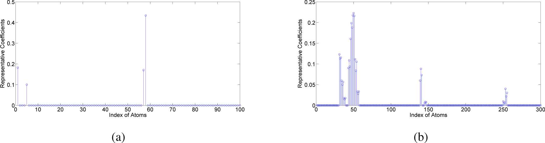
For illustration, typical sparse representative coefficients of a testing sample are shown in Figure 1a. Each class has 10 neighboring atoms as its representative in the dictionary. Four atoms out of 100 atoms are selected to represent the given sample. From Figure 1a, we can find that the largest coefficients belong to the 6th class, so the representative residual of the 6th will be smallest, and the testing sample will be assigned to the 6th class.

The approach above, named Stein-SRC, is able to give accurate classification. However, Lasso is employed for every pixel, and this will raise the computational complexity. Simplified Stein-SRC is proposed as a simplified version of the Stein-SRC above. It is a compromise scheme, in which only one atom is used instead of a group of atoms. Simplified Stein-SRC searches a training sample maximizing the Stein kernel product with the testing sample. It markedly reduces the computational complexity at the expense of a little loss of accuracy, which is appreciated in some real-time applications.

3.2. Multi-Band Merged Polarimetric SAR Classification Based on Simultaneous Sparse Representation

There are two significant directions for SAR remote sensing. One is multi-polarization; the other is multi-frequency band merging. Multi-band polarimetric SAR combines these two important directions and contains abundant information of the target. Information from different bands complements each other. The wavelength of the P, L and C bands is about 68 cm, 24 cm and 5.7 cm, respectively. Because the scattering property depends on the wavelength of the electromagnetic wave, the classification results of these three bands have significant differences. If we merge the information gathered by SAR with these three bands appropriately, it is quite probable to achieve good performance.

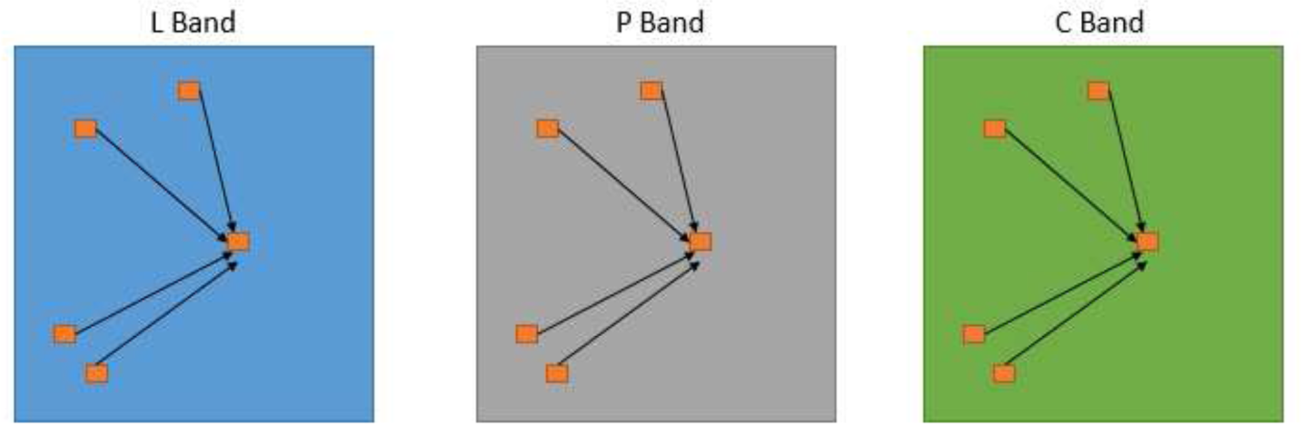
On the basis of Section 3.1, polarimetric SAR classification based on SRC can be generalized to a multi-band scenario. We assume that the representative atoms of a chosen test sample on different bands are inclined to come from the same pixel position, or the same land cover, if the polarimetric SAR image on different bands has been perfectly preprocessed by registration. If, on an L-band image, a test sample chooses the training sample at the j-th position as its atom, this means that this test sample and the j-th position training sample are quite alike. Then, on a P band image, the test sample from the same position is likely to be like the training sample from the j-th position, and it tends to choose that corresponding training sample as its atom. This is illustrated in Figure 2.

Therefore, the representative coefficients v_L on the L band, v_P on the P band, v_C on the C band tend to share the same position of non-zero entries. As mentioned by Lee [3], polarimetric SAR images of different bands can be considered as statistically independent if the radar frequencies are sufficiently separated. Our objective is to minimize the following optimization function Equation (22).

$$\underset{V_L,V_P,V_C}{\arg \min }{\Vert \varphi \left(\left[\begin{array}{l}{\mathbf{X}}_L\\ {\mathbf{X}}_P\\ {\mathbf{X}}_C\end{array}\right]\right)-\varphi \left(\left[\begin{array}{ccc}{\mathbf{D}}_{\mathbf{L}}& 0& 0\\ 0& {\mathbf{D}}_P& 0\\ 0& 0& {\mathbf{D}}_C\end{array}\right]\left[\begin{array}{l}{\mathbf{v}}_L\\ {\mathbf{v}}_P\\ {\mathbf{v}}_C\end{array}\right]\right)\Vert }_2^2+\lambda {\Vert \left[{\mathbf{v}}_L{\mathbf{v}}_P{\mathbf{v}}_C\right]\Vert }_{0-row}$$

(22)

In the equation above, X_L, X_P, X_C stands for L, P and C bands SAR data of the test sample, respectively. D_L, D_P, D_C represent the dictionaries from the training samples of the L, P and C bands, respectively. The pseudo 0-norm ${\Vert \cdot \Vert }_{0-row}$ records the number of the non-zero rows of the matrix, which can be relaxed as follows according to [19]:

$$J_{p,q}(\mathbf{C})={\displaystyle \sum _i{\Vert {\mathbf{C}}_{i,-}\Vert }_q^p}with{\Vert {\mathbf{C}}_{i,-}\Vert }_q={\left({\displaystyle \sum _j{\left|{\mathbf{C}}_{i,j}\right|}^q}\right)}^{1/q}$$

(23)

Normally, p = 1, q = 2. Let v_i represent the i-th row of the matrix, meaning that v_i= [v_Li v_Pi v_Ci]. Then, Equation (22) can be relaxed to a new form as follows.

$$\underset{V_L,V_P,V_C}{\arg \min }{\Vert \varphi \left(\left[\begin{array}{l}{\mathbf{X}}_L\\ {\mathbf{X}}_P\\ {\mathbf{X}}_C\end{array}\right]\right)-\varphi \left(\left[\begin{array}{ccc}{\mathbf{D}}_{\mathbf{L}}& 0& 0\\ 0& {\mathbf{D}}_P& 0\\ 0& 0& {\mathbf{D}}_C\end{array}\right]\left[\begin{array}{l}{\mathbf{v}}_L\\ {\mathbf{v}}_P\\ {\mathbf{v}}_C\end{array}\right]\right)\Vert }_2^2+\lambda {\displaystyle \sum _i{\Vert {\mathbf{v}}_i\Vert }_2}$$

(24)

This equation is equivalent to,

$$\underset{{\mathbf{V}}_L,{\mathbf{V}}_P,{\mathbf{V}}_C}{\arg \min }3-2{\left[\begin{array}{l}{\mathbf{v}}_L\\ {\mathbf{v}}_P\\ {\mathbf{v}}_C\end{array}\right]}^T\left[\begin{array}{l}{\mathbf{K}}_L\\ {\mathbf{K}}_P\\ {\mathbf{K}}_C\end{array}\right]+{\left[\begin{array}{l}{\mathbf{v}}_L\\ {\mathbf{v}}_P\\ {\mathbf{v}}_C\end{array}\right]}^T\left[\begin{array}{ccc}{\mathbf{K}}_L& 0& 0\\ 0& {\mathbf{K}}_P& 0\\ 0& 0& {\mathbf{K}}_C\end{array}\right]\left[\begin{array}{l}{v}_L\\ v_P\\ v_C\end{array}\right]+\lambda {\displaystyle \sum _i{\Vert {\mathbf{v}}_i\Vert }_2}$$

(25)

where κ_L, κ_P, κ_C are the kernels between the given test sample and all of the training sample atoms on the L band, P band and C bands, respectively, and K_L, K_P, K_C are the kernels among the training sample atoms on the L band, P band and C bands, respectively. Some rows and columns are then permuted in transformation as Equations (26) and (27), in which ⊗ denotes the Kronecker product. Letting v_G = [v₁ v₂ ⋯ v_m]^T, in which m denotes the number of atom groups, Equation (25) turns out to be a standard simultaneous sparse representation problem Equation (28), which can be solved by the group-lasso algorithm [19,20].

$${\mathbf{K}}_G={\mathbf{K}}_L\otimes \left[\begin{array}{ccc}1& 0& 0\\ 0& 0& 0\\ 0& 0& 0\end{array}\right]+{\mathbf{K}}_P\otimes \left[\begin{array}{ccc}0& 0& 0\\ 0& 1& 0\\ 0& 0& 0\end{array}\right]+{\mathbf{K}}_L\otimes \left[\begin{array}{ccc}0& 0& 0\\ 0& 0& 0\\ 0& 0& 1\end{array}\right]$$

(26)

$${\kappa }_G={\kappa }_L\otimes \left[\begin{array}{l}1\\ 0\\ 0\end{array}\right]+{\kappa }_P\otimes \left[\begin{array}{l}0\\ 1\\ 0\end{array}\right]+{\kappa }_C\otimes \left[\begin{array}{l}0\\ 0\\ 1\end{array}\right]$$

(27)

$$\underset{v_G}{\arg \min }3-2{\mathbf{v}}_G^T{\kappa }_G+{\mathbf{v}}_G^T{\mathbf{K}}_G{\mathbf{v}}_G+\lambda {\displaystyle \sum _i{\Vert {\mathbf{v}}_i\Vert }_2}$$

(28)

A typical representative coefficient of a testing sample using the above simultaneous Stein-SRC approach is shown in Figure 1b. The indexes of atoms corresponding to the L, P and C bands data of a training sample are neighboring, so 3 consecutive atoms form a simultaneous group. In addition, 10 consecutive groups belong to a certain class. The representative coefficient groups minimizing Equation (25) are selected. In Figure 1b, most of the largest coefficients belong to the 2nd class, which means that the representative residual of the 2nd class is the smallest, and the testing sample is assigned to the 2nd class.

In addition, in view of the computing burden of group lasso on every pixel in simultaneous Stein-SRC, a simplified version of simultaneous Stein-SRC is devised analogous to the simplified Stein-SRC, which pursues algorithm efficiency at the expense of some accuracy. In simplified simultaneous Stein-SRC, only one group of atoms is involved to represent the testing sample, and the group corresponding to the smallest residual is selected. The test sample will be assigned to the class to which the representative atoms belong.

4. Results and Discussion

4.1. Classification of Polarimetric SAR

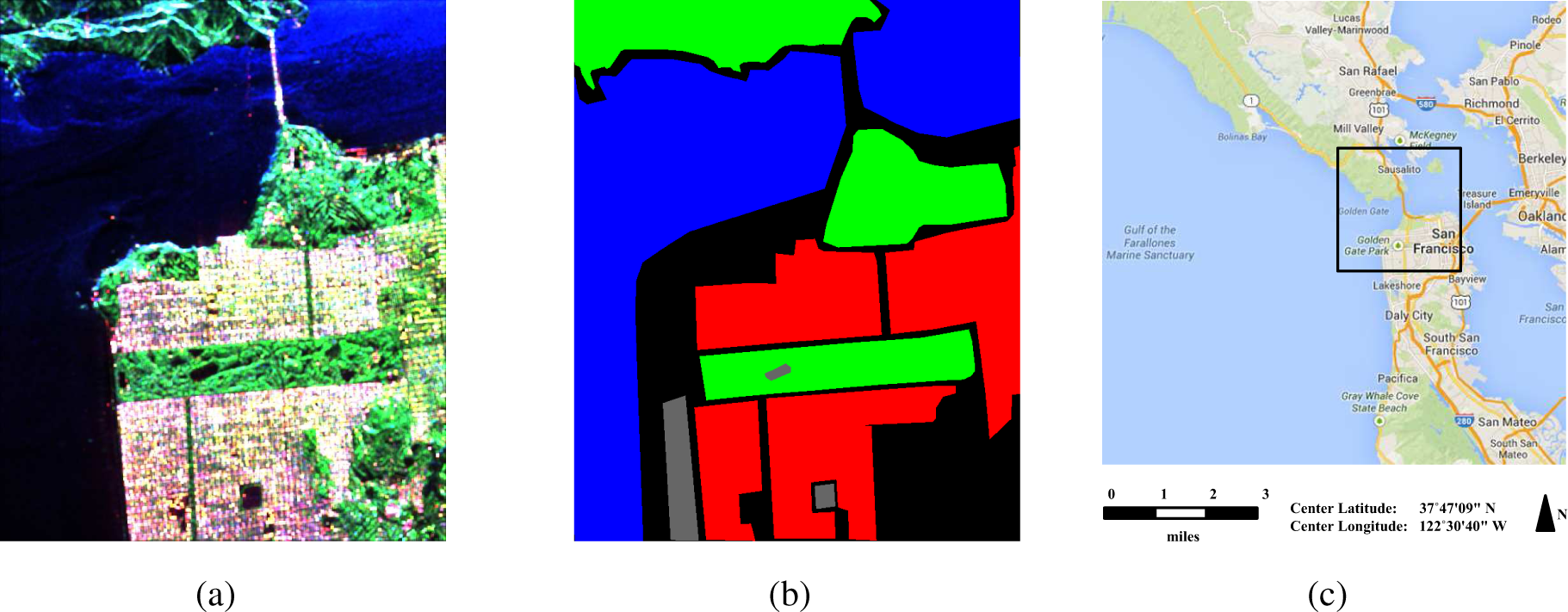
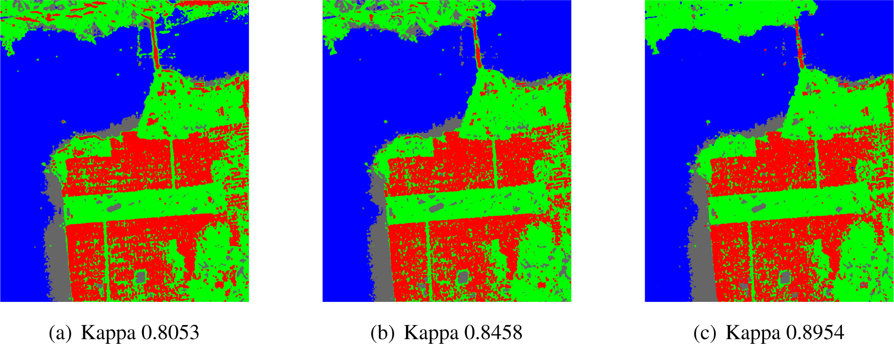
First, the San Francisco data from JPL AIRSAR have been employed for supervised classification. These data are from JPL AIRSAR, and they are in Stokes Multilook Complex (STK-MLC) format. The peuodo-color image, ground truth, and geographic information are shown in Figure 3. The ground truth is observed from the Google Earth map. One can also find the data and ground truth mentioned in a series of articles, such as [26]. There are mainly four types of land cover: sea, urban areas, forests and bare ground. From each type, 1000 pixels are randomly selected as training samples, leaving the remaining data as testing samples. Results of three methods are compared here as illustrated in Figure 4: the traditional Wishart classifier, Stein-SRC and the simplified Stein-SRC approach as proposed in Section 3. From the visualized classification results, we can find that the Wishart classifier does not perform well and confuses the top-right sea area with urban area and forest. That is probably because the Wishart classifier mainly relies on span-related information, and the span of the top-right sea area is closer to that of the urban or forest area than to bottom-left sea area; as is shown in Figure 3a, the top-right sea area is quite brighter than the bottom-left sea area. In contrast, Stein-SRC manages to solve this problem and give more accurate results. The Kappa coefficient is employed to assess the results quantitatively, which confirms the better performance of the Stein-SRC approaches. The Stein-SRC approach obtains the best performance, which is not only indicated by the Kappa coefficient, but also can be seen manually. The top-left forest areas have a wide range of scattering intensity because of the difference of incident angles due to mountainous terrain, some of which is so dark, that they are classified as sea or bare ground by Wishart. On the contrary, Stein-SRC copes with the top-left pixels very well and achieves better performance. In addition, simplified Stein-SRC, which efficiently reduces the computing burden, performs better than the Wishart classifier, as well. The concrete classification result is shown in

Table 1. Comparison of classifiers for the San Francisco image. OA, overall accuracy.

Classifier	Classification Rate (%)				OA (%)
	Ocean	Urban	Forest	Soil
Wishart	94.5	76.0	85.9	95.7	87.0
Simplified Stein SRC	99.6	77.5	87.1	97.4	90.0
Stein SRC	99.7	82.1	95.1	96.8	93.3

, from which we can get the same conclusion.

4.2. Classification of Multi-Frequency Polarimetric SAR

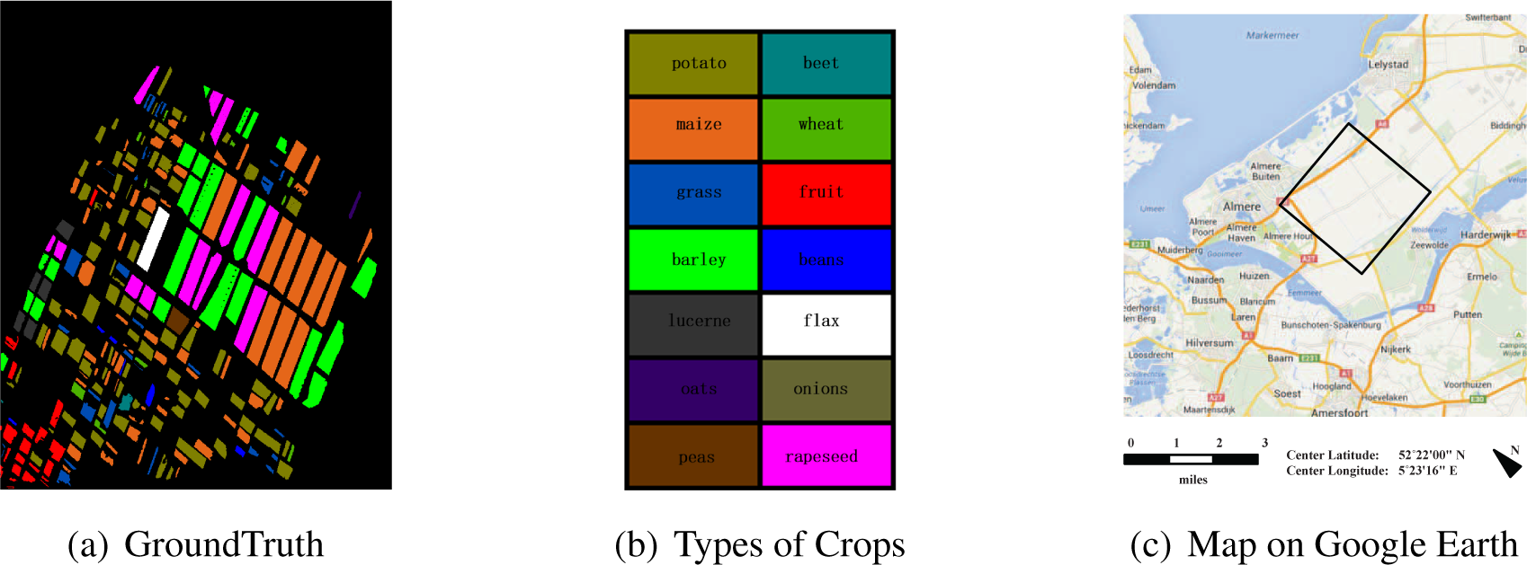
Classification experiments are run on a set of multi-look, multi-frequency polarimetric SAR images in STK-MLC format acquired by the AIRSAR sensor with the P, L and C bands over a cultivated area of Flevoland in the Netherlands in June, 1991. According to the ground-truth data provided by Hoekman [27] and Gao [7], there are mainly 14 types of crops in the scene: potato, beet, maize, wheat, grass, fruit, barley, beans, lucerne, flax, oats, onions, peas and rapeseed. The ground-truth data used in this experiment is visualized in Figure 5. From most types of crops, 1000 pixels are randomly selected as training samples, with the remaining data as testing samples. Because of comparatively less points available in the ground truth, for beet and beans, 500 pixels are randomly chosen; for oats and onions, 200 and 100 pixels are randomly selected, respectively. The Wishart classifier is employed for comparison using various combinations of the P, L and C bands images.

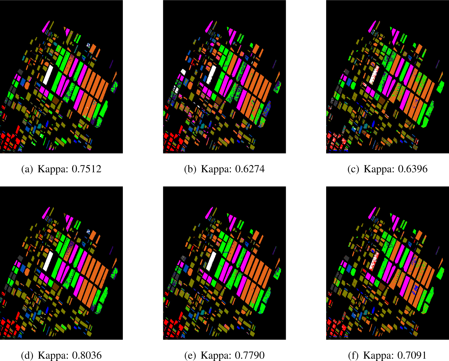
At first, single-band data are used to assess the performance of Stein-SRC and the Wishart classifier. Classification results of the L, P, and C bands data are illustrated in Figure 6. Each experiment exhibits that Stein-SRC possesses an overwhelming advantage over the Wishart classifier. On the P band, overall accurate rates are markedly raised for almost every type of crops, especially for potato, grass, barley and lucerne. On the L band, overall accurate rates are also enhanced for almost every class of crops, particularly for wheat and beans. On the C band, classification performance is improved, as well, especially for potato, wheat, grass and fruit.

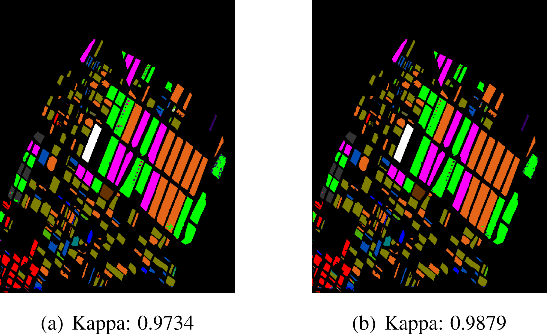
Then, the L, P and C bands data are combined in simultaneous Stein-SRC. The Wishart classifier is employed as a comparison. The classification results are shown in Figure 7.

Quantitative analysis of these approaches is given below. For most types of crops, 1000 pixels are randomly selected as training samples, and another 1000 pixels are randomly selected as testing samples. For beet, beans, oats and onions, the training and testing number of pixels is adjusted to 500, 500, 200 and 100, respectively. An average of 100 realizations is shown in

Table 2. Classification results for the Flevoland image; an average of 100 realizations. BD, band; OA, overall accuracy; Kappa coefficient.

BD	Classification Rate (%)														OA (%)	Kappa (%)
	1	2	3	4	5	6	7	8	9	10	11	12	13	14
	63.8	96.5	89.6	67.0	54.9	98.6	36.3	62.3	33.8	95.4	83.8	90.8	99.3	98.4	76.5	74.7
P	86.8	96.4	88.4	79.8	82.0	96.7	68.0	63.5	90.7	96.2	87.8	95.8	99.3	99.0	87.8	86.8
	94.9	99.7	85.8	36.1	79.7	88.7	83.7	64.5	91.2	99.9	97.9	100	100	92.4	86.7	85.7
L	96.6	99.3	92.1	68.9	94.9	91.5	85.1	76.7	98.9	99.9	98.0	100	100	98.9	92.9	92.4
	77.0	90.7	84.7	43.7	57.4	45.1	63.6	92.6	87.1	77.5	83.9	100	98.5	99.9	78.7	77.0
C	89.2	84.6	83.5	62.2	68.6	67.6	74.7	95.3	98.7	75.2	84.1	100	97.0	100	84.3	83.1
	96.1	96.7	97.1	45.6	94.4	98.4	82.1	72.5	88.1	99.9	94.9	98.4	100	99.7	90.3	89.5
PL	97.7	97.3	96.0	91.5	97.1	98.6	91.0	86.2	99.8	100	99.8	100	100	100	96.8	96.5
	94.7	96.7	98.5	81.0	89.1	98.8	71.2	95.3	77.2	99.1	86.8	97.1	99.8	100	91.8	91.2
PC	96.8	97.2	99.5	97.0	89.3	99.8	88.4	98.9	97.1	100	90.2	99.8	100	100	96.7	96.3
	98.6	99.9	94.8	42.8	82.9	91.2	95.8	92.7	95.8	100	97.8	100	100	100	92.3	91.7
LC	99.0	99.7	98.1	92.2	95.8	94.2	94.4	94.7	99.0	100	98.3	100	100	100	97.5	97.3
	99.0	97.5	99.4	86.8	94.9	98.6	93.9	89.3	94.7	100	94.6	99.7	100	99.9	96.3	96.1
PLC	98.5	98.8	98.6	99.4	98.7	99.8	99.3	94.0	99.5	100	98.8	100	100	100	99.0	98.9

. For each combination of frequency bands, the overall accurate rate and Kappa coefficients of two methods are recorded. From top to bottom are the results of the Wishart classifier and Stein-SRC. It is explicitly shown that Stein-SRC performs better than the Wishart classifier under all configurations. For the P, L and C bands, compared to the Wishart classifier, Stein-SRC improves the overall accuracy rate by 11.3%, 6.3% and 5.6%.

For most types of crops, classification on L band data is superior to that on other bands, owing to the property of electromagnetic waves. P band waves have good penetration into vegetation, but their wavelengths are too long to discriminate between similar crops. Experiments show that P band data are only more suitable to identify maize, wheat, and fruit. C band waves have too short wavelengths, which means limited penetrating ability, so the volume scattering is not fully detected. C band data achieve the best performance only for beans and rapeseed. L band waves are a good compromise, with a blend of abilities of penetration and discrimination. Different frequency bands are suitable for different types of crops. It is obvious that merging multiple bands for classification enhances the overall accuracy, since the information provided by different bands is complementary. With merging the Wishart classifier treated as a comparison reference, simultaneous Stein-SRC enhances the Kappa coefficient by 2.7%. The overall accurate rate for Stein-SRC is 99.0%, which is a quite excellent result. When only information of two bands is merged, the performances of all of these approaches fall in between those involving the three bands and the ones involving only a single band. Under any configuration of these combinations, one can find that Stein-SRC out competes the Wishart classifier.

In order to further assess the performance of the proposed approaches above, the nearest neighbor version of the Wishart classifier is employed as a reference. The Wishart distance between the testing pixel and every training pixel is calculated instead of the Wishart distance between the testing pixel and the class center. The testing pixel is assigned to the same class with the closest neighbor in the training sample set. Simplified revised Stein-SRC, which reduces the computational burden of revised Stein-SRC, is also tested as a reference. An experiment of the same configuration with the aforementioned one is undertaken, and the results are recorded in

Table 3. Classification results for the Flevoland image; an average of 100 realizations. Approaches: Wishart; nearest neighbor (NN) Wishart; simplified Stein-SRC; Stein-SRC; OA, overall accuracy; Kappa coefficient.

Approach	Classification Rate (%)														OA (%)	Kappa (%)
	1	2	3	4	5	6	7	8	9	10	11	12	13	14
Wishart	99.0	97.5	99.4	86.8	94.9	98.6	93.9	89.3	94.7	100	94.6	99.7	100	99.9	96.3	96.1
NN Wishart	99.1	98.4	99.2	94.8	95.1	98.9	98.7	93.4	97.4	100	95.7	99.9	100	100	97.9	97.8
Simplified Stein-SRC	98.1	97.8	99.1	95.5	98.1	97.8	97.4	93.5	100	99.1	99.0	100	98.8	100	98.2	98.1
Stein-SRC	98.5	98.8	98.6	99.4	98.7	99.8	99.3	94.0	99.5	100	98.8	100	100	100	99.0	98.9

. All of these approaches combine the data from the P, L and C bands. The experiment results further confirm the effectiveness of Stein-SRC approaches.

The computing time of these approaches was recorded, as well. The MATLAB codes were all executed on a platform of Intel i7-3537U 2.00 GHz. The running time for traditional Wishart classification was 141.66 s, which was the shortest due to its simplicity. The NN Wishart method consumed 1131.64 s, while the simplified version of Stein-SRC took only 526.26 s. Not only did the latter achieve better performance, but also simplified Stein-SRC expended less time, probably because it computed the matrix determinant instead of the matrix inversion in Wishart distance. Stein-SRC took the longest, 3187.28 s, because of the complex and time-consuming execution of the Lasso algorithm for each pixel. Despite the cost of efficiency, Stein-SRC achieved the best performance.

4.3. Comparisons to More Advanced Classifiers

To fully assess the performance of Stein-SRC, comparisons to more recently proposed advanced classifiers are employed in the following experiment. These classifiers include the K-Wishart model derived from the scale mixture of Gaussian (SMoG) distribution of scattering vectors [28,29], the Wishart–Kotz model from the Kotz-type distribution of scattering vectors [30] and the mixed Gaussian model by Gao [7]. Stein divergence combined with KNN k-Nearest Neighbors) instead of SRC is also included, in this experiment, K = 6. Quite similar to Stein SRC, SRC combined with kernels of geodesic distance is employed, as well.

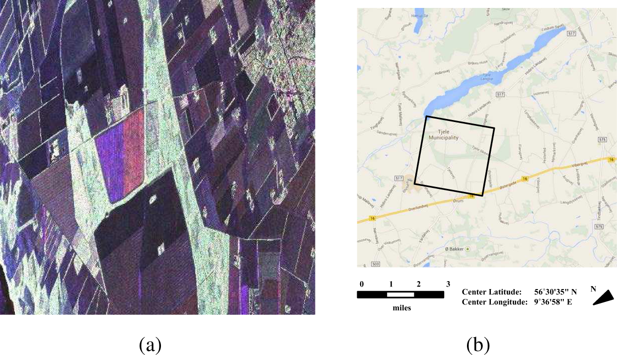
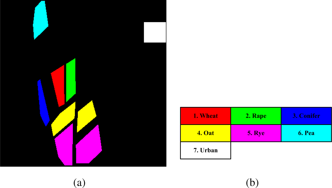
Classification is performed on a polarimetric SAR image in 3×3 complex covariance format acquired by the EMISAR sensor over the Foulum area in Denmark, which mainly contains seven types of land covers. The pseudo-color image and ground-truth data [7,31] are portrayed in Figures 8 and 9, respectively. A 3 × 3 boxcar filtering is undertaken as preprocessing. Classification results are listed in

Table 4. Comparison of classifiers for the Foulum image; an average of 100 realizations. OA, overall accuracy.

Classifier	Classification Rate (%)							OA (%)
	1	2	3	4	5	6	7
Wishart	98.1	99.9	94.3	99.7	93.2	95.0	79.4	94.2
K-Wishart	98.0	99.9	93.9	89.4	93.7	95.7	89.6	94.3
Wishart–Kotz	98.5	99.9	92.2	98.7	92.8	96.5	90.6	95.6
Wishart Mixture	99.1	100.0	94.5	99.6	94.7	97.0	82.8	95.4
Stein-KNN	98.9	100.0	95.7	100.0	95.5	96.1	82.1	95.5
geodesic-SRC	99.4	100.0	92.6	100	94.4	96.8	89.3	96.1
Stein-SRC	99.4	100.0	92.8	100.0	94.2	96.8	89.2	96.1

for each classifier, with underlined figures indicating the best classification rates and overall accuracy. The Wishart classifier can be regarded as the baseline classifier.

We can find that Stein-SRC attains the best performance on most types of land cover. It is noteworthy that the Wishart classifier does not perform well, especially on Class 7, urban areas, because it is modeled for homogeneous regions. Wishart–Kotz and K-Wishart are able to classify the urban areas very well, because they are modeled to describe heterogeneous regions, but they do not fit the crop area very well. Stein-SRC is flexible and achieve the highest overall accuracy, because it does not depend on much of a distribution assumption. Moreover, ENL (equivalent number of looks) must be estimated exactly as the parameter of the models to maintain the performance of Wishart–Kotz and K-Wishart. Once ENL estimation is not correct, the performance deteriorates obviously. In contrast, Stein-SRC does not need ENL as a parameter and does not have this problem. Finally, the more complicated the distribution model is, the more parameters are needed to be estimated. If the training samples are insufficient, the estimation of these parameters is inaccurate, and hence, the performance turns worse significantly. For example, the Wishart mixture model does not work if the training sample is inadequate. On the other hand, the performance of Stein-SRC does not decline much even though the number of training samples decreases. The Stein-KNN method attains the best performance on many types of land cover. However, it fails to classify urban areas well. The performance of geodesic-SRC is almost as good as that of Stein-SRC, because Stein divergence is approximate to geodesic distance. Nevertheless, it takes more time to compute geodesic distance than Stein divergence. In our experiment, 35.2 s was spent for every one million times of computing geodesic distance, while only 16.4 s was spent for the same amount of times of computing Stein divergence.

The influence of kernel parameter σ was also discussed. The overall accuracy when σ equals 0.5, 1, 2 and 5 is 96.09%, 96.09%, 96.23% and 96.06%, respectively. Therefore, the choice of σ does not affect the performance much. In the experiments above, normally σ = 1.

5. Conclusions

In this paper, Stein-SRC approach has been proposed to classify polarimetric SAR data. This approach was based on SRC in sparse representation and Stein divergence on the Riemannian manifold of a Hermitian semidefinite matrix, such as a covariance and a coherency matrix. In addition, it was generalized to simultaneous Stein-SRC for multi-frequency merging applications, on the basis of the assumption that different frequency data are independent and tend to have similar forms of sparse representation. Experiments on single-band AIRSAR data of San Francisco confirmed the effectiveness of the Stein-SRC approach, which gave much better classification results compared to the Wishart classifier, especially for the class spanning a wide range of scattering intensity. Experiments on multi-band AIRSAR data of Flevoland showed that not only Stein-SRC performed better by using L, P and C band data separately, but also simultaneous Stein-SRC worked better by using arbitrary combinations of these multi-frequency data. Further comparison to more advanced models was undertaken on the EMISAR sensor over the Foulum area in Denmark. Qualitative and quantitative analysis both confirmed the better effectiveness of Stein-SRC and simultaneous Stein-SRC.

References

- Kong, J.A.; Swartz, A.A.; Yueh, H.A.; Novak, L.M.; Shin, R.T. Identification of terrain cover using the optimum polarimetric classifier. J. Electromagn. Waves Appl. 1987, 2, 171–194. [Google Scholar]
- Lim, H.H.; Swartz, A.A.; Yueh, H.A.; Kong, J.A.; Shin, R.T. Classification of earth terrain using polarimetric synthetic aperture radar images. J. Geophys. Res. 1989, 94, 7049–7057. [Google Scholar]
- Lee, J.S.; Grunes, M.R.; Kwok, R. Classification of multi-look polarimetric SAR imagery based on complex Wishart distribution. Int. J. Remote Sens. 1994, 15, 2299–2311. [Google Scholar]
- Greco, M.S.; Gini, F. Statistical analysis of high-resolution SAR ground clutter data. IEEE Trans. Geosci. Remote Sens. 2007, 45, 566–575. [Google Scholar]
- Vasile, G.; Ovarlez, J; Pascal, F.; Tison, C. Coherency matrix estimation of heterogeneous clutter in high-resolution polarimetric SAR images. IEEE Trans. Geosci. Remote Sens. 2010, 48, 1809–1826. [Google Scholar]
- Bombrun, L.; Vasile, G.; Gay, M.; Totir, F. Hierarchical segmentation of polarimetric SAR images using heterogeneous clutter models. IEEE Trans. Geosci. Remote Sens. 2011, 49, 726–737. [Google Scholar]
- Gao, W.; Yang, J.; Ma, W. Land cover classification for polarimetric SAR images based on mixture models. Remote Sens. 2014, 6, 3770–3790. [Google Scholar]
- Dong, Y.; Milne, A.K.; Forster, B.C. Segmentation and classification of vegetated areas using polarimetric SAR image data. IEEE Trans. Geosci. Remote Sens. 2001, 39, 321–329. [Google Scholar]
- Wu, Y.; Ji, K.; Yu, W.; Su, Y. Region-based classification of polarimetric SAR images using Wishart MRF. IEEE Geosci. Remote Sens. Lett. 2008, 5, 668–672. [Google Scholar]
- Wang, Y.; Han, C. PolSAR image segmentation by mean shift clustering in the tensor space. Acta Autom. Sin. 2010, 6, 798–806. [Google Scholar]
- Song, H.; Yang, W.; Xu, X.; Liao, M. Unsupervised PolSAR Imagery Classification Based On Jensen-Bregman LogDet Divergence, Proceedings of the 10th European Conference on Synthetic Aperture Radar, Berlin, Germany, 3–5 June 2014; pp. 915–918.
- Pennec, X.; Fillard, P.; Ayache, N. A Riemannian framework for tensor computing. Int. J. Comput. Vis. 2006, 66, 41–66. [Google Scholar]
- Arsigny, V.; Fillard, P.; Pennec, X.; Ayache, N. Log-Euclidean metrics for fast and simple calculus on diffusion tensors. Magn. Reson. Med. 2006, 56, 411–421. [Google Scholar]
- Sra, S. Positive definite matrices and the symmetric Stein divergence, 2012. arXiv:1110.1773. arXiv.org e-Print archive. Available online: http://arxiv.org/abs/1110.1773 accessed on 1 July 2015.
- Wright, J.; Yang, A.Y.; Ganesh, A.; Sastry, S.S.; Yi, M. Robust face recognition via sparse representation. IEEE Trans. Pattern Anal. Mach. Intell. 2009, 31, 210–227. [Google Scholar]
- Xu, B.; Cui, Y.; Li, Z.; Zuo, B.; Yang, J.; Song, J. Patch ordering based SAR image despeckling via transform-domain filtering. IEEE J. Sel. Top. Appl. Earth Observ. Remote Sens. 2015, 8, 1682–1695. [Google Scholar]
- Zhang, L.; Sun, L.; Zhou, B.; Moon, W. Fully polarimetric SAR image classification via sparse representation and polarimetric features. IEEE J. Sel. Top. Appl. Earth Observ. Remote Sens. 2014, 1–10. [Google Scholar]
- Harandi, M.T.; Sanderson, C.; Sanderson, C.; Hartley, R.; Lovell, B.C. Sparse Coding and Dictionary Learning for Symmetric Positive Definite Matrices: A Kernel Approach, Proceedings Part II of the 12th European Conference on Computer Vision, Florence, Italy, 7–13 October 2012; pp. 216–229.
- Rakotomamonjy, A. Surveying and comparing simultaneous sparse approximation (or group lasso) algorithms. Signal Process. 2011, 91, 1505–1526. [Google Scholar]
- Yuan, M.; Lin, Y. Model selection and estimation in regression with grouped variables. R. Stat. Soc. B 2006, 68, 49–67. [Google Scholar]
- Goodman, N.R. Statistical analysis based on a certain multivariate complex Gaussian distribution (An introduction). Ann. Math. Stat. 1963, 34, 152–177. [Google Scholar]
- Cherian, A.; Sra, S.; Banerjee, A.; Papanikolopoulos, N. Jensen-bregman logdet divergence with application to efficient similarity search for covariance matrices. IEEE Trans. Pattern Anal. Mach. Intell. 2012, 35, 2161–2174. [Google Scholar]
- Conradsen, K.; Nielsen, A.; Schou, J.; Skriver, H. A test statistic in the complex Wishart distribution and its application to change detection in polarimetric SAR data. IEEE Trans. Geosci. Remote Sens. 2003, 41, 4–19. [Google Scholar]
- Chen, S.; Donoho, D.; Saunders, M.A. Atomic decomposition by basis pursuit. SIAM Rev. 2001, 43, 129–159. [Google Scholar]
- Tibshirani, R. Regression shrinkage and selection via the LASSO. R. Stat. Soc. B 1996, 58, 267–288. [Google Scholar]
- Lee, J.; Grunes, M.R.; Ainsworth, T.L.; Du, L.; Schuler, D.L.; Cloude, S.R. Unsupervised Classification Using Polarimetric Decomposition and the Complex Wishart Classifier. IEEE Trans. Geosci. Remote Sens. 1999, 37, 2249–2258. [Google Scholar]
- Hoekman, D.H.; Vissers, M.A.M. A new polarimetric classification approach evaluated for agricultural crops. IEEE Trans. Geosci. Remote Sens. 2003, 41, 2881–2889. [Google Scholar]
- Doulgeris, A.P.; Anfinsen, S.N.; Eltoft, T. Classification with a non-Gaussian model for PolSAR data. IEEE Trans. Geosci. Remote Sens. 2008, 46, 2999–3009. [Google Scholar]
- Doulgeris, A.P.; Anfinsen, S.N.; Eltoft, T. Automated non-Gaussian clustering of polarimetric synthetic aperture radar images. IEEE Trans. Geosci. Remote Sens. 2011, 49, 3665–3676. [Google Scholar]
- Kersten, P.R.; Anfinsen, S.N.; Doulgeris, A.P. The Wishart-Kotz Classifier for Multilook Polarimetric SAR Data, Proceedings of the IEEE International Geoscience and Remote Sensing Symposium, Munich, Germany, 22–27 July 2012; pp. 3146–3149.
- Skriver, H.; Dall, J.; le Toan, T.; Quegan, S.; Ferro-Famil, L.; Pottier, E.; Lumsdon, P.; Moshammer, R. Agriculture Classification Using PolSAR Data, Proceedings of the 2nd International Workshop on Science and Applications of SAR Polarimetry and Polarimetric Interferometry, Frascati, Italy, 17–21 January 2005; pp. 213–218.