
Evaluation of Polarimetric SAR Decomposition for Classifying Wetland Vegetation Types

Abstract
:
1. Introduction
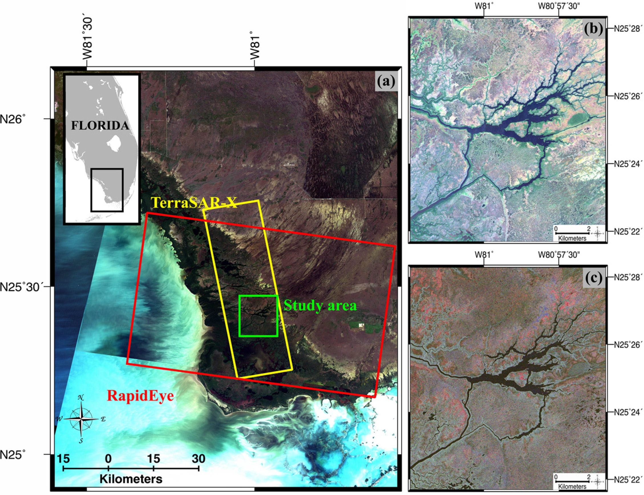
2. Study Area

3. Data

| TerraSAR-X | RapidEye | ||
|---|---|---|---|
| Acquisition date | 16 April 2010 | Acquisition date | 03 December 2010 |
| Wavelength | 3.1 cm | Spectral bands | |
| Carrier frequency | X-band (9.6 GHz) | Blue | 440–510 nm |
| Pulse repetition frequency | 2950 Hz | Green | 520–590 nm |
| ADC sampling rate | 164.8 MHz | Red | 630–685 nm |
| Polarization | Quad-pol | Red Edge | 690–730 nm |
| Flight direction | Ascending | Near Infrared (NIR) | 760–850 nm |
| Incidence angle | 32.6 deg | Incidence angle | 7.11 deg |
| Azimuth pixel spacing | 2.40 m | Geometric resolution | 6.5 m (resampled 5 m) |
| Range pixel spacing | 0.91 m | Dynamic range | 12 bits |

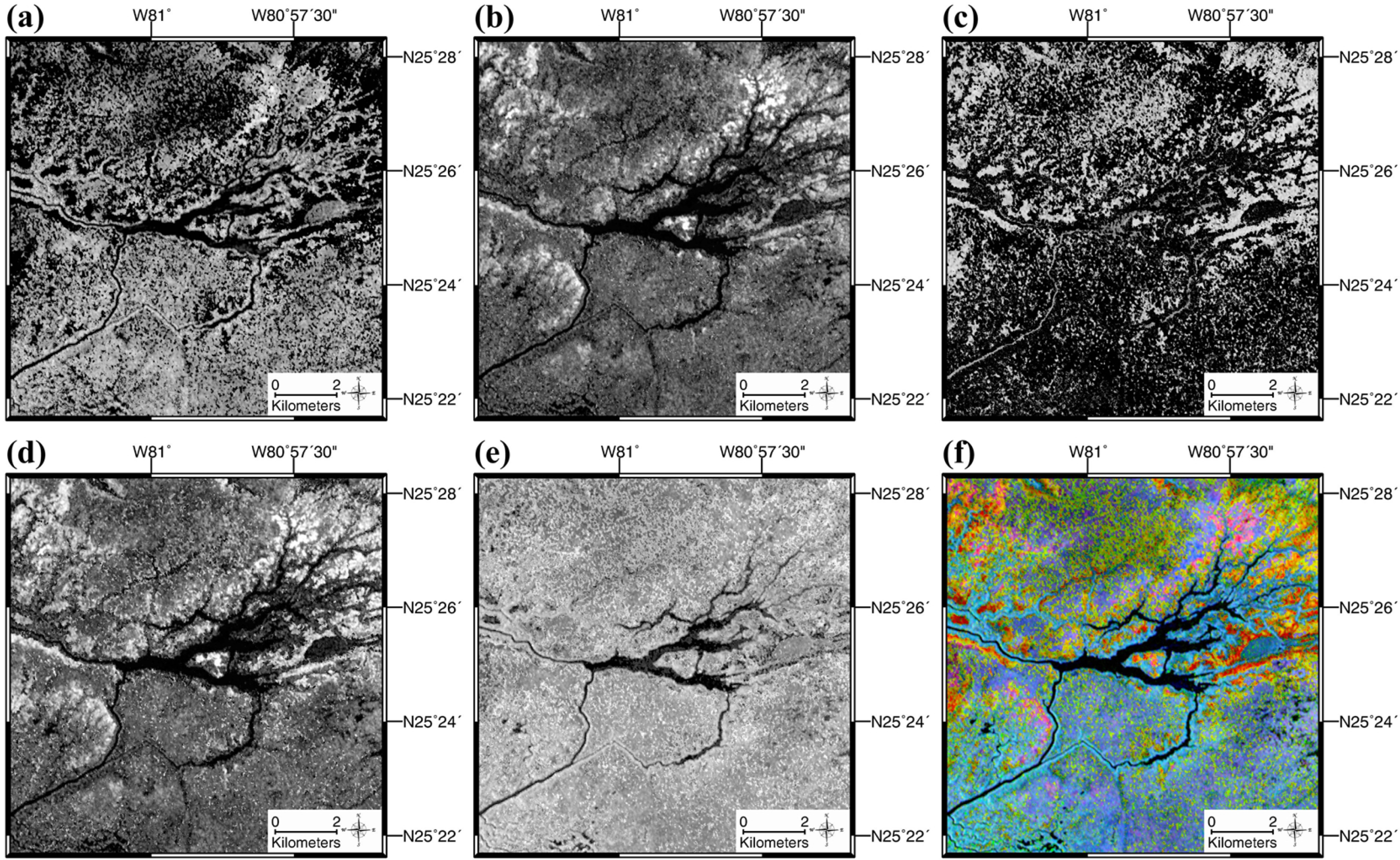
4. SAR Decomposition

5. Vegetation Changes in Everglades and Selection of Vegetation Types


6. Wetland Vegetation Classification
6.1. Method
| Segmentation Type | Image Source | Image Layer | Scale | Shape | Compactness |
|---|---|---|---|---|---|
| Type O | RapidEye | Blue, Green, Red, Red-Edge, NIR, NDVI | 50 | 0.1 | 0.5 |
| Type S | TSX | Single, Double, Double from co-pol, Double from cross-pol, Volume | 50 | 0.1 | 0.5 |
| Type M | TSX & RapidEye | Blue, Green, Red, Red-Edge, NIR, NDVI, Single, Double, Double from co-pol, Double from cross-pol, Volume | 50 | 0.1 | 0.5 |
| Scenario | Image Layer Features Used for Classification (Mean Object Value) | Segmentation Type |
|---|---|---|
| Scenario 1 | RapidEye’s blue, green, red, red-edge, NIR, and NDVI | Type O |
| Scenario 2 | RapidEye’s blue, green, red, red-edge, NIR and NDVI & TerraSAR-X’s single, double, double from co-pol, double from cross-pol, and volume | Type O |
| Scenario 3 | TerraSAR-X’s single, double, double from co-pol, double from cross-pol, and volume | Type O |
| Scenario 4 | TerraSAR-X’s single, double, double from co-pol, double from cross-pol, and volume | Type S |
| Scenario 5 | TerraSAR-X’s single, double, volume and helix using the Yamaguchi decomposition | Type O |
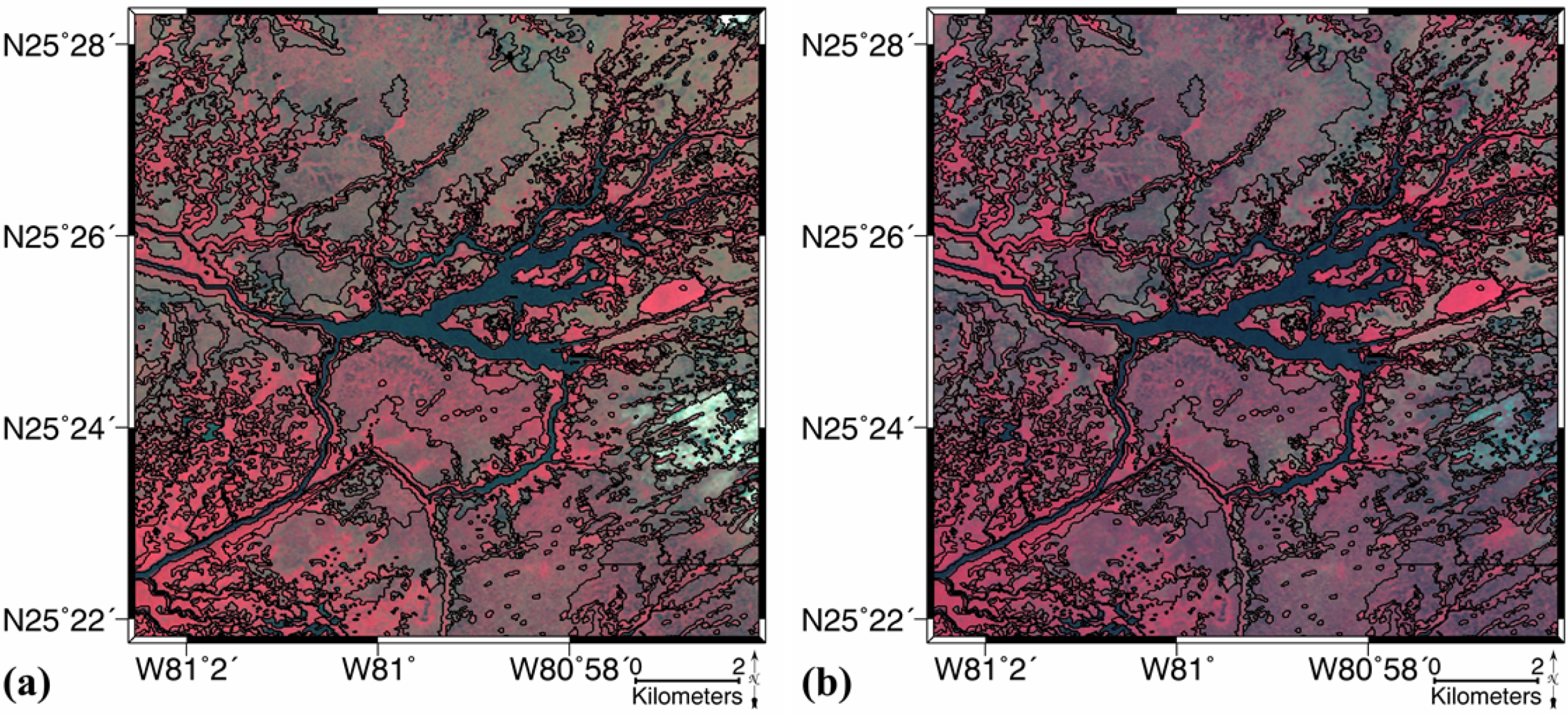
6.2. Segmentation Results

6.3. Classification Results and Accuracy Assessment

| Scenario 1 | ||||||
|---|---|---|---|---|---|---|
| Reference | ||||||
| F | S | P | W | PA (%) | ||
| class | F | 22 | 100.0 | |||
| S | 25 | 100.0 | ||||
| P | 21 | 100.0 | ||||
| W | 0.0 | |||||
| N | 3 | |||||
| UA | 100.0 | 100.0 | 100.0 | 0.0 | ||
| OA | 95.8 | |||||
| Scenario 2 | ||||||
| Reference | ||||||
| F | S | P | W | PA (%) | ||
| class | F | 21 | 1 | 95.5 | ||
| S | 1 | 24 | 2 | 88.9 | ||
| P | 18 | 100.0 | ||||
| W | 0.0 | |||||
| N | 1 | 3 | ||||
| UA | 95.5 | 96.0 | 85.7 | 0.0 | ||
| OA | 88.7 | |||||
| Scenario 3 | ||||||
| Reference | ||||||
| F | S | P | W | PA (%) | ||
| class | F | 22 | 1 | 95.6 | ||
| S | 24 | 1 | 1 | 92.3 | ||
| P | 1 | 20 | 1 | 90.9 | ||
| W | 0.0 | |||||
| N | ||||||
| UA | 100.0 | 96.0 | 95.2 | 0.0 | ||
| OA | 93.0 | |||||
| Scenario 4 | ||||||
| Reference | ||||||
| F | S | P | W | PA (%) | ||
| class | F | 21 | 1 | 1 | 1 | 87.5 |
| S | 1 | 22 | 1 | 1 | 88.0 | |
| P | 1 | 19 | 1 | 90.5 | ||
| W | 1 | 0.0 | ||||
| N | ||||||
| UA | 95.5 | 88.0 | 90.5 | 0.0 | ||
| OA | 87.3 | |||||
| Scenario 5 | ||||||
| Reference | ||||||
| F | S | P | W | PA (%) | ||
| class | F | 20 | 3 | 2 | 1 | 76.9 |
| S | 2 | 22 | 1 | 1 | 84.6 | |
| P | 18 | 1 | 94.7 | |||
| W | 0.0 | |||||
| N | ||||||
| UA | 90.9 | 88.0 | 85.7 | 0.0 | ||
| OA | 84.5 | |||||
7. Discussion and Conclusions
Acknowledgments
Author Contributions
Conflicts of Interest
References
- Center for International Forestry Research (CIFOR). Tropical Wetlands Initiative: For Climate Adaptation and Mitigation; CIFOR: Bogor, Indonesia, 2012. [Google Scholar] [CrossRef]
- Barbier, E.B. Valuing environmental functions: Tropical wetlands. Land Econ. 1994. [Google Scholar] [CrossRef]
- Madden, M.; Jones, D.; Vilchek, L. Photointerpretation key for the everglades vegetation classification system. Photogramm. Eng. Remote Sens. 1999, 65, 171–177. [Google Scholar]
- Rutchey, K.; Vilchek, L. Air photointerpretation and satellite imagery analysis techniques for mapping cattail coverage in a northern everglades impoundment. Photogramm. Eng. Remote Sens. 1999, 65, 185–191. [Google Scholar]
- Rutchey, K.; Schall, T.; Sklar, F. Development of vegetation maps for assessing everglades restoration progress. Wetlands 2008, 28, 806–816. [Google Scholar] [CrossRef]
- Hirano, A.; Madden, M.; Welch, R. Hyperspectral image data for mapping wetland vegetation. Wetlands 2003, 23, 436–448. [Google Scholar] [CrossRef]
- Zhang, C.; Xie, Z. Combining object-based texture measures with a neural network for vegetation mapping in the everglades from hyperspectral imagery. Remote Sens. Environ. 2012, 124, 310–320. [Google Scholar] [CrossRef]
- Fuller, D. Remote detection of invasive melaleuca trees (Melaleuca quinquenervia) in South Florida with multispectral IKONOS imagery. Int. J. Remote Sens. 2005, 26, 1057–1063. [Google Scholar] [CrossRef]
- Hess, L.L.; Melack, J.M.; Simonett, D.S. Radar detection of flooding beneath the forest canopy: A review. Int. J. Remote Sens. 1990, 11, 1313–1325. [Google Scholar] [CrossRef]
- Ramsey, E.; Rangoonwala, A.; Bannister, T. Coastal flood inundation monitoring with satellite C-band and L-band Synthetic Aperture Radar data. J. Am. Water Resour. Assoc. 2013, 49, 1239–1260. [Google Scholar] [CrossRef]
- Alsdorf, D.E.; Melack, J.M.; Dunne, T.; Mertes, L.A.K.; Hess, L.L.; Smith, L.C. Interferometric radar measurements of water level changes on the Amazon flood plain. Nature 2000, 404, 174–177. [Google Scholar] [CrossRef] [PubMed]
- Wdowinski, S.; Amelung, F.; Miralles-Wilhelm, F.; Dixon, T.H.; Carande, R. Space-based measurements of sheet-flow characteristics in the everglades wetland, Florida. Geophys. Res. Lett. 2004, 31. [Google Scholar] [CrossRef]
- Wdowinski, S.; Kim, S.W.; Amelung, F.; Dixon, T.H.; Miralles-Wilhelm, F.; Sonenshein, R. Space-based detection of wetlands’ surface water level changes from L-band SAR interferometry. Remote Sens. Environ. 2008, 112, 681–696. [Google Scholar] [CrossRef]
- Hong, S.-H.; Wdowinski, S.; Kim, S.-W. Evaluation of TERRASAR-X observations for wetland InSAR application. IEEE Trans. Geosci. Remote Sens. 2010, 48, 864–873. [Google Scholar] [CrossRef]
- Ramsey, I.; Elijah; Lu, Z.; Rangoonwala, A.; Rykhus, R. Multiple baseline radar interferometry applied to coastal land cover classification and change analyses. GISci. Remote Sens. 2006, 43, 283–309. [Google Scholar] [CrossRef]
- Yamagata, Y.; Yasuoka, Y. Classification of wetland vegetation by texture analysis methods using ERS-1 and JERS-1 images. In Proceedings of the IEEE International Conference on Geoscience and Remote Sensing Symposium, Tokyo, Japan, 18–21 August 1993; pp. 1614–1616.
- Kasischke, E.S.; Bourgeau-Chavez, L.L. Monitoring South Florida wetlands using ERS-1 SAR imagery. Photogramm. Eng. Remote Sens. 1997, 63, 281–291. [Google Scholar]
- Hess, L.L.; Melack, J.M.; Novo, E.M.; Barbosa, C.C.; Gastil, M. Dual-season mapping of wetland inundation and vegetation for the central Amazon Basin. Remote Sens. Environ. 2003, 87, 404–428. [Google Scholar] [CrossRef]
- Martinez, J.-M.; Le Toan, T. Mapping of flood dynamics and spatial distribution of vegetation in the amazon floodplain using multitemporal SAR data. Remote Sens. Environ. 2007, 108, 209–223. [Google Scholar] [CrossRef]
- Evans, T.L.; Costa, M. Landcover classification of the lower nhecolândia subregion of the Brazilian pantanal wetlands using ALOS/PALSAR, RADARSAT-2 and ENVISAT/ASAR imagery. Remote Sens. Environ. 2013, 128, 118–137. [Google Scholar] [CrossRef]
- Bourgeau-Chavez, L.L.; Riordan, K.; Powell, R.B.; Miller, N.; Nowels, M. Improving wetland characterization with multi-sensor, multi-temporal SAR and optical/infrared data fusion. In Advances in Geosci. Remote Senssing; InTech: Rijeka, Croatia, 2009. [Google Scholar]
- Baghdadi, N.; Bernier, M.; Gauthier, R.; Neeson, I. Evaluation of C-band SAR data for wetlands mapping. Int. J. Remote Sens. 2001, 22, 71–88. [Google Scholar] [CrossRef]
- Touzi, R. Wetland characterization using polarimetric RADARSAT-2 capability. In Proceedings of the IEEE International Conference on Geoscience and Remote Sensing Symposium, Denver, CO, USA, 31 July–4 August 2006; pp. 1639–1642.
- Touzi, R.; Deschamps, A.; Rother, G. Phase of target scattering for wetland characterization using polarimetric C-band sar. IEEE Trans. Geosci. Remote Sens. 2009, 47, 3241–3261. [Google Scholar] [CrossRef]
- Brisco, B.; Kapfer, M.; Hirose, T.; Tedford, B.; Liu, J. Evaluation of C-band polarization diversity and polarimetry for wetland mapping. Can. J. Remote Sens. 2011, 37, 82–92. [Google Scholar] [CrossRef]
- Brisco, B.; Schmitt, A.; Murnaghan, K.; Kaya, S.; Roth, A. SAR polarimetric change detection for flooded vegetation. Int. J. Digit. Earth 2013, 6, 103–114. [Google Scholar] [CrossRef]
- Cloude, S.R.; Pottier, E. A review of target decomposition theorems in radar polarimetry. IEEE Trans. Geosci. Remote Sens. 1996, 34, 498–518. [Google Scholar] [CrossRef]
- ESA. Polsarpro. Available online: http://earth.esa.int/polsarpro/ (accessed on 10 June 2015).
- Freeman, A.; Durden, S.L. A three-component scattering model for polarimetric SAR data. IEEE Trans. Geosci. Remote Sens. 1998, 36, 963–973. [Google Scholar] [CrossRef]
- Yamaguchi, Y.; Moriyama, T.; Ishido, M.; Yamada, H. Four-component scattering model for polarimetric SAR image decomposition. IEEE Trans. Geosci. Remote Sens. 2005, 43, 1699–1706. [Google Scholar] [CrossRef]
- Yamaguchi, Y.; Yajima, Y.; Yamada, H. A four-component decomposition of polsar images based on the coherency matrix. IEEE Geosci. Remote Sens. Lett. 2006, 3, 292–296. [Google Scholar] [CrossRef]
- Yamaguchi, Y.; Sato, A.; Boerner, W.M.; Sato, R.; Yamada, H. Four-component scattering power decomposition with rotation of coherency matrix. IEEE Trans. Geosci. Remote Sens. 2011, 49, 2251–2258. [Google Scholar] [CrossRef]
- Lee, J.S.; Ainsworth, T.L. The effect of orientation angle compensation on coherency matrix and polarimetric target decompositions. IEEE Trans. Geosci. Remote Sens. 2011, 49, 53–64. [Google Scholar] [CrossRef]
- van Zyl, J.J.; Arii, M.; Kim, Y. Model-based decomposition of polarimetric SAR covariance matrices constrained for nonnegative eigenvalues. IEEE Trans. Geosci. Remote Sens. 2011, 49, 3452–3459. [Google Scholar]
- Atwood, D.; Leinss, S.; Matthiss, B.; Jenkins, L.; Wdowinski, S.; Hong, S.-H. Wave propagation model for coherent scattering from a randomly distributed target. In Proceedings of POLinSAR 2013 Workshop, Frascati, Italy, 28 January–1 February 2013.
- Hong, S.H.; Wdowinski, S. Double-bounce component in cross-polarimetric SAR from a new scattering target decomposition. IEEE Trans. Geosci. Remote Sens. 2014, 52, 3039–3051. [Google Scholar] [CrossRef]
- Wdowinski, S.; Hong, S.-H. Tropical wetland characterization with polarimetry SAR. In Proceedings of 9th Advanced SAR Workshop (ASAR), Longueuil, QC, Canada, 15–18 October 2013.
- Florida Coastal Everglades Long Term Ecological Research. Available online: http://fcelter.fiu.edu (accessed on 9 June 2015).
- Global Land Cover Facility. Available online: http://www.landcover.org/data/landsat (accessed on 9 June 2015).
- Cibula, W.; Carter, G. Identification of a FAR-red reflectance response to ectomycorrhizae in slash pine. Int. J. Remote Sens. 1992, 13, 925–932. [Google Scholar] [CrossRef]
- Filella, I.; Penuelas, J. The red edge position and shape as indicators of plant chlorophyll content, biomass and hydric status. Int. J. Remote Sens. 1994, 15, 1459–1470. [Google Scholar] [CrossRef]
- Kim, H.-O.; Yeom, J.-M. Effect of red-edge and texture features for object-based paddy rice crop classification using rapideye multispectral satellite image data. J. Remote Sens. 2014, 35, 7046–7068. [Google Scholar]
- Schuster, C.; Förster, M.; Kleinschmit, B. Testing the red edge channel for improving land-use classifications based on high-resolution multi-spectral satellite data. Int. J. Remote Sens. 2012, 33, 5583–5599. [Google Scholar] [CrossRef]
- Tigges, J.; Lakes, T.; Hostert, P. Urban vegetation classification: Benefits of multitemporal rapideye satellite data. Remote Sens. Environ. 2013, 136, 66–75. [Google Scholar] [CrossRef]
- Welch, R.; Madden, M.; Doren, R.F. Mapping the everglades. Photogramm. Eng. Remote Sens. 1999, 65, 163–170. [Google Scholar]
- Cloude, S. Polarisation: Applications in Remote Sensing; Oxford University Press: New York, NY, USA, 2010. [Google Scholar]
- Lee, J.S.; Pottier, E. Polarimetric Radar Imaging: From Basics to Applications; CRC: Boca Raton, FL, USA, 2009; Volume 142. [Google Scholar]
- Neumann, M.; Ferro-Famil, L.; Pottier, E. A general model-based polarimetric decomposition scheme for vegetated areas. In Proceedings of POLinSAR 2009 Workshop, Frascati, Italy, 26–30 January 2009.
- Arii, M.; van Zyl, J.J.; Kim, Y. A general characterization for polarimetric scattering from vegetation canopies. IEEE Trans. Geosci. Remote Sens. 2010, 48, 3349–3357. [Google Scholar] [CrossRef]
- Arii, M.; van Zyl, J.J.; Kim, Y. Adaptive model-based decomposition of polarimetric SAR covariance matrices. IEEE Trans. Geosci. Remote Sens. 2011, 49, 1104–1113. [Google Scholar] [CrossRef]
- Sato, A.; Yamaguchi, Y.; Singh, G.; Park, S.E. Four-component scattering power decomposition with extended volume scattering model. IEEE Geosci. Remote Sens. Lett. 2012, 9, 166–170. [Google Scholar] [CrossRef]
- Hong, S.-H.; Wdowinski, S. Evaluation of the quad-polarimetric RADARSAT-2 observations for the wetland InSAR application. Can. J. Remote Sens. 2012, 37, 484–492. [Google Scholar] [CrossRef]
- Rignot, E.; Chellappa, R.; Dubois, P. Unsupervised segmentation of polarimetric SAR data using the covariance matrix. IEEE Trans. Geosci. Remote Sens. 1992, 30, 697–705. [Google Scholar] [CrossRef]
- Chen, K.; Huang, W.; Tsay, D.; Amar, F. Classification of multifrequency polarimetric SAR imagery using a dynamic learning neural network. IEEE Trans. Geosci. Remote Sens. 1996, 34, 814–820. [Google Scholar] [CrossRef]
- Chen, C.-T.; Chen, K.-S.; Lee, J.-S. The use of fully polarimetric information for the fuzzy neural classification of SAR images. IEEE Trans. Geosci. Remote Sens. 2003, 41, 2089–2100. [Google Scholar] [CrossRef]
- Dong, Y.; Milne, A.K. Segmentation and classification of vegetated areas using polarimetric SAR image data. IEEE Trans. Geosci. Remote Sens. 2001, 39, 321–329. [Google Scholar] [CrossRef]
- Lombardo, P.; Sciotti, M.; Pellizzeri, T.M.; Meloni, M. Optimum model-based segmentation techniques for multifrequency polarimetric SAR images of urban areas. IEEE Trans. Geosci. Remote Sens. 2003, 41, 1959–1975. [Google Scholar] [CrossRef]
- Benz, U.C.; Hofmann, P.; Willhauck, G.; Lingenfelder, I.; Heynen, M. Multi-resolution, object-oriented fuzzy analysis of remote sensing data for GIS-ready information. ISPRS J. Photogramm. Remote Sens. 2004, 58, 239–258. [Google Scholar] [CrossRef]
- Luscier, J.D.; Thompson, W.L.; Wilson, J.M.; Gorham, B.E.; Dragut, L.D. Using digital photographs and object-based image analysis to estimate percent ground cover in vegetation plots. Front. Ecol. Environ. 2006, 4, 408–413. [Google Scholar] [CrossRef]
- Mathieu, R.; Freeman, C.; Aryal, J. Mapping private gardens in urban areas using object-oriented techniques and very high-resolution satellite imagery. Landsc. Urban Plan. 2007, 81, 179–192. [Google Scholar] [CrossRef]
- Neubert, M.; Herold, H.; Meinel, G. Assessing image segmentation quality—Concepts, methods and application. In Object-Based Image Analysis; Springer: Berlin, Germany, 2008; pp. 769–784. [Google Scholar]
- Blaschke, T. Object based image analysis for remote sensing. ISPRS J. Photogramm. Remote Sens. 2010, 65, 2–16. [Google Scholar] [CrossRef]
- Qi, Z.; Yeh, A.G.-O.; Li, X.; Lin, Z. A novel algorithm for land use and land cover classification using RADARSAT-2 polarimetric SAR data. Remote Sens. Environ. 2012, 118, 21–39. [Google Scholar] [CrossRef]
- Ehlers, M.; Gaehler, M.; Janowsky, R. Automated techniques for environmental monitoring and change analyses for ultra high resolution remote sensing data. Photogramm. Eng. Remote Sens. 2006, 72, 835–844. [Google Scholar] [CrossRef]
- Kim, H.-O.; Kleinschmit, B.; Kenneweg, H. High resolution satellite imagery for the analysis of sealing in the metropolitan area seoul. Remote Sens. GIS Environ. Stud.: Appl. Geogr. 2005, 113, 281. [Google Scholar]
- Ecognition. Available online: http://www.ecognition.com (accessed on 10 June 2015).
- Trimble. About classification; Ecognition Developer 8.64.0: User Guide; Trimble Germany Gmbh: Muenchen, Germany, 2010; pp. 106–123. [Google Scholar]
- Brisco, B.; Ahern, F.; Hong, S.-H.; Wdowinski, S.; Murnaghan, K.; White, L.; Atwood, D.K. Polarimetric decompositions of temperate wetlands at C-band. IEEE J. Sel. Top. Appl. Earth Obs. Remote Sens. 2015. [Google Scholar] [CrossRef]
- Lucas, R.M.; Mitchell, A.L.; Rosenqvist, A.; Proisy, C.; Melius, A.; Ticehurst, C. The potential of L-band SAR for quantifying mangrove characteristics and change: Case studies from the tropics. Aquat. Conserv.: Mar. Freshw. Ecosyst. 2007, 17, 245–264. [Google Scholar] [CrossRef]
- Mougin, E.; Proisy, C.; Marty, G.; Fromard, F.; Puig, H.; Betoulle, J.; Rudant, J.-P. Multifrequency and multipolarization radar backscattering from mangrove forests. IEEE Trans. Geosci. Remote Sens. 1999, 37, 94–102. [Google Scholar] [CrossRef]
- Trisasongko, B.H. Tropical mangrove mapping using fully-polarimetric radar data. J. Math. Funda. Sci. 2009, 41, 98–109. [Google Scholar] [CrossRef]
- Adam, E.; Mutanga, O.; Rugege, D. Multispectral and hyperspectral remote sensing for identification and mapping of wetland vegetation: A review. Wetl. Ecol. Manag. 2010, 18, 281–296. [Google Scholar] [CrossRef]
- Kamal, M.; Phinn, S.; Johansen, K. Object-based approach for multi-scale mangrove composition mapping using multi-resolution image datasets. Remote Sens. 2015, 7, 4753–4783. [Google Scholar] [CrossRef]
- Zhang, C.; Kovacs, J.M.; Liu, Y.; Flores-Verdugo, F.; Flores-de-Santiago, F. Separating mangrove species and conditions using laboratory hyperspectral data: A case study of a degraded mangrove forest of the Mexican Pacific. Remote Sens. 2014, 6, 11673–11688. [Google Scholar] [CrossRef]
- Heenkenda, M.K.; Joyce, K.E.; Maier, S.W.; Bartolo, R. Mangrove species identification: Comparing Worldview-2 with aerial photographs. Remote Sens. 2014, 6, 6064–6088. [Google Scholar] [CrossRef]
© 2015 by the authors; licensee MDPI, Basel, Switzerland. This article is an open access article distributed under the terms and conditions of the Creative Commons Attribution license (http://creativecommons.org/licenses/by/4.0/).
Share and Cite
Hong, S.-H.; Kim, H.-O.; Wdowinski, S.; Feliciano, E. Evaluation of Polarimetric SAR Decomposition for Classifying Wetland Vegetation Types. Remote Sens. 2015, 7, 8563-8585. https://doi.org/10.3390/rs70708563
Hong S-H, Kim H-O, Wdowinski S, Feliciano E. Evaluation of Polarimetric SAR Decomposition for Classifying Wetland Vegetation Types. Remote Sensing. 2015; 7(7):8563-8585. https://doi.org/10.3390/rs70708563
Chicago/Turabian StyleHong, Sang-Hoon, Hyun-Ok Kim, Shimon Wdowinski, and Emanuelle Feliciano. 2015. "Evaluation of Polarimetric SAR Decomposition for Classifying Wetland Vegetation Types" Remote Sensing 7, no. 7: 8563-8585. https://doi.org/10.3390/rs70708563