Reconstruction of Satellite-Retrieved Land-Surface Reflectance Based on Temporally-Continuous Vegetation Indices

Abstract

Land-surface reflectance, estimated from satellite observations through atmospheric corrections, is an essential parameter for further retrieval of various high level land-surface parameters, such as leaf area index (LAI), fraction of absorbed photosynthetically active radiation (FAPAR), and surface albedo. Although great efforts have been made, land-surface reflectance products still contain considerable noise caused by, e.g., cloud or mixed-cloud pixels, which results in temporal and spatial inconsistencies in subsequent downstream products. In this study, a new method is developed to remove the residual clouds in the Moderate Resolution Imaging Spectroradiometer (MODIS) land-surface reflectance product and reconstruct time series of surface reflectance for the red, near infrared (NIR), and shortwave infrared (SWIR) bands. A smoothing method is introduced to calculate upper envelopes of vegetation indices (VIs) from the surface reflectance data and the cloud contaminated reflectance data are identified using the time series VIs and the upper envelopes of the time series VIs. Surface reflectance was then reconstructed according to cloud-free surface reflectance by incorporating the upper envelopes of the time series VIs as constraint conditions. The method was applied to reconstruct time series of surface reflectance from MODIS/TERRA surface reflectance product (MOD09A1). Temporal consistency analysis indicates that the new method can reconstruct temporally-continuous time series of land-surface reflectance. Comparisons with cloud-free MODIS/AQUA surface reflectance product (MYD09A1) over the BELMANIP (Benchmark Land Multisite Analysis and Intercomparison of Products) sites in 2003 demonstrate that the new method provides better performance for the red band (R² = 0.8606 and RMSE = 0.0366) and NIR band (R² = 0.6934 and RMSE = 0.0519), than the time series cloud detection (TSCD) algorithm (R² = 0.5811 and RMSE = 0.0649; and R² = 0.5005 and RMSE = 0.0675, respectively).

1. Introduction

Land-surface reflectance is an essential parameter to describe properties on the Earth’s surface. Many higher level products, such as leaf area index (LAI), fraction of absorbed photosynthetically-active radiation (FAPAR), and surface albedo, are often derived from surface reflectance data [1].

Multiple global land-surface reflectance products have been generated from data acquired by the Moderate-Resolution Imaging Spectroradiometer (MODIS) [2], Multiangle Imaging SpectroRadiometer (MISR) and VEGETATION. These products were retrieved from top-of-atmosphere (TOA) reflectance data after correcting for various atmospheric effects on the TOA signal. Since clouds preclude the detection of land surface and atmospheric aerosols scatter and absorb the incoming radiation, no reliable retrieval can be achieved in the presence of clouds, cloud shadows, high atmospheric aerosol content, or at high solar zenith angles [3]. Therefore, the quality and character of surface reflectance depends on the accuracy of the cloud mask and aerosol algorithms.

Many methods have been developed to detect cloud-contaminated pixels in TOA reflectance data based on spatial, spectral, and temporal information [4,5,6]. The subsequent quality of the corrected surface reflectance data was greatly improved. However, residual clouds or undetected cloud shadows are observed in surface reflectance products, which always results in temporal and spatial inconsistencies in subsequent downstream products. The cloud or cloud shadow detection remains quite challenging.

Earlier studies often estimated land-surface parameters using vegetation indices (VIs), so various methods were developed to reconstruct VI time series data [7,8]. Now, as more algorithms use individual band reflectance, the accurate retrieval of surface reflectance becomes increasingly important [9]. For example, almost all of the canopy radiative transfer models that are used for inverting land surface biophysical parameters are based on surface reflectance. Therefore, it is urgent to refine cloud detection procedures of surface reflectance data and reconstruct time series of surface reflectance. Liu & Liu [10] proposed an inflexion based cloud detection algorithm to generate cloud masks based on time series of surface reflectance in the blue band, and the ratios between surface reflectance in visible and shortwave infrared (SWIR) bands from MODIS/TERRA surface reflectance product (MOD09A1). Comparisons show that, generally, this cloud detection algorithm performs better than the cloud masks accompanying the MOD09A1 product. However, the method just identifies cloud-contaminated reflectance values. It does not remove cloud contamination nor fill in missing reflectance values.

Based on the relative stability of ground reflectance and the sudden variations in TOA reflectance that result from cloud cover, Tang et al. [11] developed a time series cloud detection (TSCD) algorithm which first searches the clear-sky reference data, and then discriminates between clouded and unclouded pixels by detecting a rapid change of surface reflectance in the blue wavelength and spectral correlation coefficient at the pixel level. The TSCD algorithm was applied to the MOD09A1 product to remove cloud contamination and fill missing pixels. Compared with cloud cover assessments obtained from MODIS cloud mask, the TSCD algorithm performs very well, particularly when the land surface is stable or changing only slowly [12].

However, these existing surface reflectance data reprocessing methods are dependent on surface reflectance in the blue band and other auxiliary information. Therefore, it is difficult to apply these methods directly to reprocess the MODIS 250 m resolution surface reflectance data (containing only red and near infrared (NIR) bands). Similarly, these methods can not be directly used to reprocess surface reflectance data from the Visible Infrared Imaging Radiometer Suite (VIIRS), which is considered as a convergence of its operational predecessor of the Advanced Very High Resolution Radiometer (AVHRR) and MODIS to provide long time series of accurate data required for global climate monitoring [13,14], because the VIIRS surface reflectance data contain only red, NIR and SWIR bands.

In this study a new method is developed to remove residual clouds in the MODIS land-surface reflectance product and reconstruct time series of surface reflectance in the red, NIR and SWIR bands based on temporally continuous VIs. Vegetation index, usually obtained by mathematical combinations of satellite observations from different spectral bands, is the most commonly used and effective parameter for characterizing vegetation cover and growth status [15]. Compared with the surface reflectance data, vegetation index exhibits obvious seasonal changes which make it relatively easy to reconstruct temporally continuous VIs. Considering the negative bias of VIs when surface reflectance values were contaminated by clouds, upper envelopes of VIs (defined as the smoothest curve that passes through all the maxima of the time series VIs) were calculated. The cloud-contaminated reflectance values were identified using the time series VIs and the upper envelopes of the time series VIs. Then, the time series of surface reflectance was reconstructed according to cloud-free surface reflectance values by incorporating the upper envelopes of the time series VIs as constraint conditions. The method was applied to reprocess the MOD09A1 product, and the results were compared with reconstruction from the TSCD algorithm and the cloud-free MODIS/AQUA surface reflectance (MYD09A1).

The organization of this paper is as follows. In Section 2, we introduce our approach for reconstructing time series of surface reflectance. This includes gap filling and smoothing of VIs, cloud detection and surface reflectance reconstruction. The MOD09A1 and MYD09A1 products used in this study are also briefly described in this section. Section 3 contains the results of reprocessed surface reflectance of MOD09A1 from our proposed method, and a comparison of our results with reprocessed surface reflectance of MOD09A1 from the TSCD algorithm and the cloud-free surface reflectance from MYD09A1. Discussions are presented in Section 4, and the final section provides brief conclusions.

2. Methodology and Data

The proposed method incorporates upper envelopes of time series VIs as constraint conditions to reconstruct time series of surface reflectance (referred to hereafter as VIRR algorithm for clarification). The flowchart of the VIRR algorithm is shown in Figure 1. Satellite-retrieved surface reflectance data are used to calculate VIs, and a robust smoothing method is used to calculate continuous and smooth upper envelopes of VIs. Cloud-contaminated surface reflectance values were detected using the time series VIs and the upper envelopes of the time series VIs. Surface reflectance data with good quality in a given time window, along with the continuous and smooth upper envelopes of VIs, were used to estimate the optimal values of control variables of fitting models to the surface reflectance data. The method tunes the control variables of the fitting models until the temporal behavior of modeled surface reflectance and VIs reach the best agreement with the multi-temporal surface reflectance data from satellites and the upper envelopes of the VIs. Then, time series of surface reflectance can be reconstructed using the fitting models according to the optimal values of the control variables. Detailed descriptions of the important parts of the VIRR algorithm are as follows.

Figure 1. Flow diagram of reconstructing time series of satellite retrieved surface reflectance data.

Figure 1. Flow diagram of reconstructing time series of satellite retrieved surface reflectance data.

2.1. Gap filling and Smoothing of Vegetation Indices

Many vegetation indices have been developed [16,17,18,19]. The most widely used index is the normalized difference vegetation index (NDVI), which is based on the difference between the maximum absorption of radiation in the red band and the maximum reflection of radiation in the NIR band. The formula to calculate the NDVI, denoted as VI^NIR,Red, is as follows

$$V{I}^{\text{NIR,Red}}=\frac{{\text{ρ}}^{\text{NIR}}-{\text{ρ}}^{\text{Red}}}{{\text{ρ}}^{\text{NIR}}+{\text{ρ}}^{\text{Red}}},$$

(1)

where ${\mathrm{\rho }}^{\mathrm{Red}}$ and ${\mathrm{\rho }}^{\mathrm{NIR}}$ are surface reflectance in the red and NIR bands, respectively. NDVI ranges from −1.0 to 1.0, and is highly correlated with vegetation parameters such as green biomass, and absorbed radiation by photosynthetically-active vegetation [20,21]. NDVI establishes the relationship between surface reflectance in the red and NIR bands. To establish the relationship between the surface reflectance in the NIR and SWIR bands, we define a new vegetation index, denoted as VI^SWIR,NIR. As with the NDVI, VI^SWIR,NIR is calculated as the normalized difference between SWIR and NIR spectral bands,

$$V{I}^{\text{SWIR,NIR}}=\frac{{\text{ρ}}^{\text{SWIR}}-{\text{ρ}}^{\text{NIR}}}{{\text{ρ}}^{\text{SWIR}}+{\text{ρ}}^{\text{NIR}}},$$

(2)

where ${\mathrm{\rho }}^{\mathrm{SWIR}}$ is the surface reflectance in the SWIR band.

As the result of atmospheric effects on surface reflectance, some VI values were missing, and there are abrupt drops in the time series of the two VIs. Time series of VIs with abrupt drops are not consistent with vegetation succession. Except in the case of disturbances (such as fires, floods, and hurricanes), VIs vary smoothly over time. Therefore, a smooth temporal course of VIs derived from remote sensing data can be expected.

A number of gap filling and smoothing methods have been developed to reduce cloud and atmospheric contamination in the time series of vegetation indices and reconstruct the vegetation's dynamic trajectory [7,22,23,24]. We used the smoothing method developed by Garcia [25] to reduce cloud and atmospheric contamination in the time series of VI^NIR,Red and VI^SWIR,NIR. The method is a penalized least square regression based on three-dimensional discrete cosine transform (DCT-PLS).

Let X be a vector that contains a series of equally spaced VI values $x_i,i=1,2,\cdots ,n$. Let W be the diagonal matrix that contains the weights, w_i, corresponding to the VI value x_i. The DCT-PLS consists in minimizing the following functional to find the best smoothing estimate, $\widehat{X}$, of X [25].

$$F\left(\widehat{X}\right)={\Vert W^{1/2}\left(\widehat{X}-X\right)\Vert }^2+s{\Vert D\widehat{X}\Vert }^2,$$

(3)

where D is the Laplace operator, and s is a real positive scalar that controls the degree of smoothing. Minimizing on $\widehat{X}$ can be achieved using an iterative procedure. With type-2 discrete cosine transform (DCT) and inverse discrete cosine transform (IDCT), the $\widehat{X}$ can be expressed as

$${\widehat{X}}_{\left\{k+1\right\}}=IDCT\left(\Gamma DCT\left(W\left(X-{\widehat{X}}_{\left\{k\right\}}\right)+{\widehat{X}}_{\left\{k\right\}}\right)\right),$$

(4)

where ${\widehat{X}}_{\left\{k\right\}}$ refers to $\widehat{X}$ calculated at the kth iteration step, and $\Gamma$ is a diagonal matrix the components

$${\Gamma }_{i,i}={\left(1+s{\left(2-2\cos \left(\left(i-1\right)\pi /n\right)\right)}^2\right)}^{-1},$$

(5)

The method provides fast smoothing of data by means of a discrete cosine transform, and is a fully automated procedure for use on uniformly sampled datasets [25]. To address missing and outlying values, an iteratively reweighted process was used to assign a low weight to high leverage points and outliers, and conversely, allocate a relatively high weight to high quality data. The process constructed weights using a specified weighting function based on the current residuals, updating them from iteration to iteration until the residuals remain unchanged [25,26]. Note that atmospheric effects on surface reflectance generally cause an increase in reflectance in the red band rather than in the NIR band, resulting in decreases in the VIs. To account for negatively biased noise, we used the weight function

$$w_i=\{\begin{array}{cc}1.0\hfill & \hfill u_i>0.0\\ {(1.0-{\left(\frac{u_i}{4.685}\right)}^2)}^2\hfill & \hfill -\text{1.0}<\frac{u_i}{4.685}<0.0\\ 0.0\hfill & \hfill \frac{u_i}{4.685}<-1.0\end{array},$$

(6)

where u_i is the studentized residual, calculated by

$$u_i=r_i{\left(1.4826\text{ MAD}\left(r\right)\sqrt{1-\frac{\sqrt{1+\sqrt{1+16s}}}{\sqrt{2}\sqrt{1+16s}}}\right)}^{-1},$$

(7)

where $r_i=x_i-{\widehat{x}}_i$ is the residual of the ith observation, and MAD denotes the median absolute deviation [27]. This iteratively reweighted procedure leads to a smoothed curve adapted to the upper envelope of the VIs in the time series.

2.2. Cloud Detection of Surface Reflectance

In this study, residual cloud contamination was detected from the seasonal trajectories of VIs described in Section 2.1 for each pixel. Atmospheric effects on surface reflectance generally cause negatively biased noise within the vegetation index values. The smoothing method described in Section 2.1 was first used to calculate the upper envelopes of VI^NIR,Red and VI^SWIR,NIR, denoted by VI_Env^NIR,Red and VI_Env^SWIR,NIR, respectively. If VI values at each time satisfy the following conditions, the surface reflectance data were deemed to be contaminated by clouds or other factors. Otherwise, they were considered to be cloud free and of high quality.

$$\left|V{I}_i^{\text{NIR,Red}}-VI\_En{v}_i^{\text{NIR,Red}}\right|>\alpha \times VI\_En{v}_i^{\text{NIR,Red}},$$

(8)

and

$$\left|V{I}_i^{\text{SWIR,NIR}}-VI\text{\_}En{v}_i^{\text{SWIR,NIR}}\right|>\alpha \times VI\text{\_}En{v}_i^{\text{SWIR,NIR}},$$

(9)

where $\text{α}$ is a threshold and was set to 0.4 in this study.

The method was applied to check the time series surface reflectance, and any data points assessed as contaminated were filtered out. Indeed, this is not a conclusive clear-sky pixel identification scheme because pixels marked as clear-sky land may still contain cloud. Any undetected contaminated pixels can still be excluded, and the missing data were filled, during subsequent processing steps.

2.3. Surface Reflectance Reconstruction

Missing surface reflectance data will result in the absence of downstream products. In this study, the time series surface reflectance was reconstructed according to the surface reflectance with high quality by incorporating the upper envelopes of the time series VIs.

Let $\left(t_i,I_i\right),i=1,2,\cdots ,m$ be a series of data points, where t_i is time, and I_i is surface reflectance in different bands. In this study, only surface reflectance in the red, NIR and SWIR bands were reconstructed. Therefore, $I_i={\left({\text{ρ}}_i^{\text{red}},{\text{ρ}}_i^{\text{NIR}},{\text{ρ}}_i^{\text{SWIR}}\right)}^T$, where ${\mathrm{\rho }}_i^{\mathrm{red}}$, ${\mathrm{\rho }}_i^{\mathrm{NIR}}$, and ${\mathrm{\rho }}_i^{\mathrm{SWIR}}$ are the surface reflectance for the i-th position in the red, NIR and SWIR bands, respectively. For each data point, I_i, a quadratic polynomial function, $f\left(t\right)=a{t}^2+bt+c$, was fitted to all 2n+1 surface reflectance values in each band in a moving window using the least squares method. An optimization method searched the trajectories of the quadratic polynomial functions that best fit the surface reflectance in the given time window, i.e., minimizing

$$\begin{array}{l}J\left(X_i\right)={\displaystyle \sum _{j=-n}^n{\left(f_{\text{red}}\left(t_{i+j}\right)-{\text{ρ}}_{i+j}^{\text{red}}\right)}^2}+{\displaystyle \sum _{j=-n}^n{\left(f_{\text{NIR}}\left(t_{i+j}\right)-{\text{ρ}}_{i+j}^{\text{NIR}}\right)}^2}+{\displaystyle \sum _{j=-n}^n{\left(f_{\text{SWIR}}\left(t_{i+j}\right)-{\text{ρ}}_{i+j}^{\text{SWIR}}\right)}^2}+\\ \hspace{1em}\hspace{1em}\hspace{1em}\hspace{1em}\hspace{1em}{\displaystyle \sum _{j=-n}^n{\left(VI\_Si{m}_{i+j}^{\text{NIR,red}}-VI\_En{v}_{i+j}^{\text{NIR,red}}\right)}^2}+{\displaystyle \sum _{j=-n}^n{\left(VI\_Si{m}_{i+j}^{\text{SWIR,NIR}}-VI\text{\_}En{v}_{i+j}^{\text{SWIR,NIR}}\right)}^2}\end{array}$$

(10)

where $f_{\mathrm{red}}\left(t_i\right)$, $f_{\mathrm{NIR}}\left(t_i\right)$, and $f_{\mathrm{SWIR}}\left(t_i\right)$ are the quadratic polynomial functions for the red, NIR, and SWIR bands, respectively; $X_i={\left(a_{\text{red}},b_{\text{red}},c_{\text{red}},a_{\text{NIR}},b_{\text{NIR}},c_{\text{NIR}},a_{\text{SWIR}},b_{\text{SWIR}},c_{\text{SWIR}}\right)}^T$ is a control variable from the coefficients of the quadratic polynomial functions; $VI\_Si{m}_i^{\text{NIR,red}}$ and $VI\_Si{m}_i^{\text{SWIR,NIR}}$ are simulated vegetation indices, which were calculated using the values of the quadratic polynomial functions; and n is the size of the moving window. In this study, n was set to 2. Then, the reconstructed surface reflectance data were set as the values of those quadratic polynomial functions at the ith position.

To minimize the objective function, $J\left(X_i\right)$, the SCE-UA algorithm was used to obtain the optimal control vector, which does not require the derivative of the function and thus avoids being trapped by small pits and bumps on the function surface. The SCE-UA search routine is a global optimization strategy that combines the strength of the simplex method with the concept of a controlled random search, competitive evolution, and the strategy of complex shuffling. The synthesis of the four concepts makes the SCE-UA method more effective, robust, flexible, and efficient, and less sensitive to the initial values of the parameters than the simplex method [28].

2.4. Data

We chose the MOD09A1 product to test the proposed VIRR method, and the cloud-free MYD09A1 product was used as reference data for evaluation of the reconstructed time series of surface reflectance. The MOD09A1/MYD09A1 products, which include seven bands (Table 1) with a 500 m spatial resolution and an eight day temporal sampling period was derived from the latest version (Collection 5) and was downloaded from http://reverb.echo.nasa.gov/reverb/. In this study, only MODIS/TEERA surface reflectance in the red (B1), NIR (B2), and SWIR (B6) bands are reconstructed for further retrieval of various land parameters.

Two tiles with different biome types (h27v05, h12v09) were selected to investigate spatial patterns specific to the reconstructed surface reflectance as well to check the distribution in space of the surface reflectance contaminated by clouds. Tile h27v05 is located in Shandong, China. The main biome type is cropland according to the MODIS land cover product (MCD12Q1). Tile h12v09 is in the Amazon, and the biome type is tropical forest according to MCD12Q1 product.

Table 1. MODIS surface reflectance bands.

No. Bands	Band Name	Band Width (nm)
B1	Red	620–670
B2	NIR	841–876
B3	Blue	459–479
B4	Green	545–565
B5	NIR	1230–1250
B6	SWIR	1628–1652
B7	SWIR	2105–2155

Table 1. MODIS surface reflectance bands.

No. Bands	Band Name	Band Width (nm)
B1	Red	620–670
B2	NIR	841–876
B3	Blue	459–479
B4	Green	545–565
B5	NIR	1230–1250
B6	SWIR	1628–1652
B7	SWIR	2105–2155

The BELMANIP (Benchmark Land Multisite Analysis and Intercomparison of Products) network, which includes 402 sites, provides a good sampling of biome types and conditions throughout the world [29]. For each BELMANIP site, a 7 × 7 subset of the reconstructed surface reflectance from the VIRR and TSCD algorithms and the surface reflectance from MYD09A1 in 2003 was extracted to evaluate the performance of the reconstructed surface reflectance.

In addition, five sites with different biome types were selected to compare the time series of surface reflectance from MOD09A1 and the reconstructed surface reflectance from the VIRR and TSCD algorithms. The five sites we chose were: Alpilles, Yucheng, Konza, Counami, Tapajos, and their attributes are shown in Table 2.

Table 2. Selected site information.

Site Name	Country	Latitude (°)	Longitude (°)	Land Cover Types
Alpilles	France	43.81	4.74	Cropland
Yucheng	China	36.95	116.60	Cropland
Konza	USA	39.08	−96.62	Grassland
Counami	French Guyana	5.34	−53.24	Evergreen broadleaf forest
Tapajos	Brazil	−2.87	−54.95	Evergreen broadleaf forest

Table 2. Selected site information.

Site Name	Country	Latitude (°)	Longitude (°)	Land Cover Types
Alpilles	France	43.81	4.74	Cropland
Yucheng	China	36.95	116.60	Cropland
Konza	USA	39.08	−96.62	Grassland
Counami	French Guyana	5.34	−53.24	Evergreen broadleaf forest
Tapajos	Brazil	−2.87	−54.95	Evergreen broadleaf forest

3. Result Analysis

The VIRR method was applied to remove residual clouds in the MOD09A1 product and reconstruct time series of surface reflectance in the red, NIR and SWIR bands. The results were compared with the reconstructed surface reflectance from the TSCD algorithm.

3.1. Comparison in Space

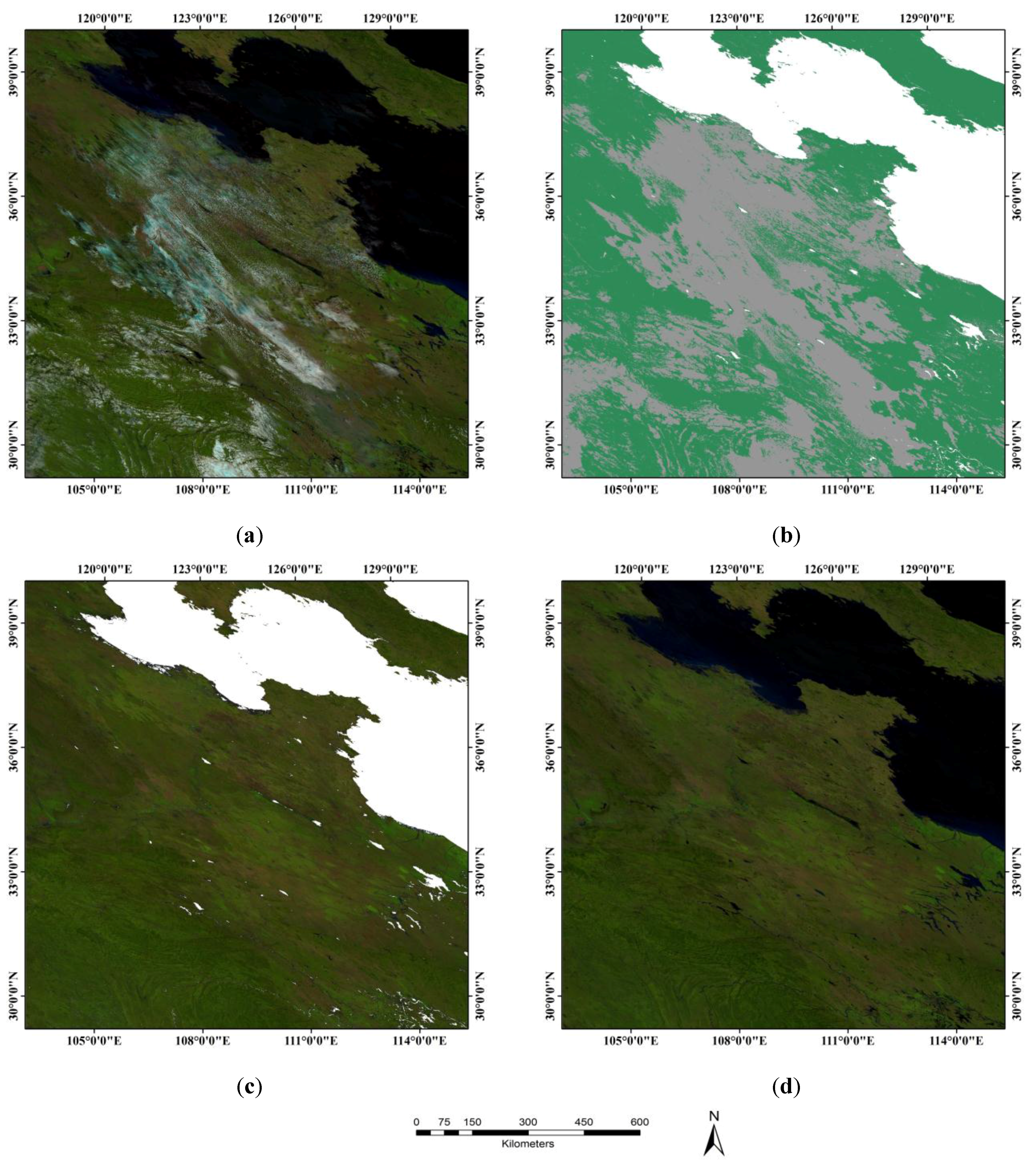
An example of cloud detection and surface reflectance reconstruction is shown in Figure 2 for tile h27v05 on day 273, 2003. Figure 2a is an RGB image of surface reflectance from MOD09A1. RGB images of the reconstructed surface reflectance data using the VIRR and TSCD methods are shown in Figure 2c,d respectively. The images were produced with an RGB color scheme that employs bands B6 (as red color), B2 (as green color), and B1 (as blue color), and the same color enhancement was used. In Figure 2a, the surface reflectance from MOD09A1 is contaminated with residual clouds, and large clouds can be visually seen over the middle area of the image. Figure 2b displays the cloud (grey) mask derived from the VIRR method. Generally, clouds in most areas can be identified by the VIRR algorithm. From the RGB image in Figure 2c,d, the VIRR and TSCD methods removed the residual clouds in the surface reflectance from MOD09A1.

Figure 2. Tile h27v05 for day 273, 2003. (a) RGB image for surface reflectance from MOD09A1; (b) cloud (grey) mask from the VIRR algorithm; (c) RGB image for reconstructed surface reflectance from the VIRR algorithm; (d) RGB image for reconstructed surface reflectance from the TSCD algorithm. The RGB images were produced with an RGB color scheme that employs bands B6 (as red color), B2 (as green color), and B1 (as blue color), and the same color enhancement was used.

Figure 2. Tile h27v05 for day 273, 2003. (a) RGB image for surface reflectance from MOD09A1; (b) cloud (grey) mask from the VIRR algorithm; (c) RGB image for reconstructed surface reflectance from the VIRR algorithm; (d) RGB image for reconstructed surface reflectance from the TSCD algorithm. The RGB images were produced with an RGB color scheme that employs bands B6 (as red color), B2 (as green color), and B1 (as blue color), and the same color enhancement was used.

Figure 3. Tile h12v09 for day 97, 2003. (a) RGB image for surface reflectance from MOD09A1; (b) cloud (grey) mask from the VIRR algorithm; (c) RGB image for reconstructed surface reflectance from the VIRR algorithm; (d) RGB image for reconstructed surface reflectance from the TSCD algorithm. The RGB images were produced with an RGB color scheme that employs bands B6 (as red color), B2 (as green color), and B1 (as blue color), and the same color enhancement was used.

Figure 3. Tile h12v09 for day 97, 2003. (a) RGB image for surface reflectance from MOD09A1; (b) cloud (grey) mask from the VIRR algorithm; (c) RGB image for reconstructed surface reflectance from the VIRR algorithm; (d) RGB image for reconstructed surface reflectance from the TSCD algorithm. The RGB images were produced with an RGB color scheme that employs bands B6 (as red color), B2 (as green color), and B1 (as blue color), and the same color enhancement was used.

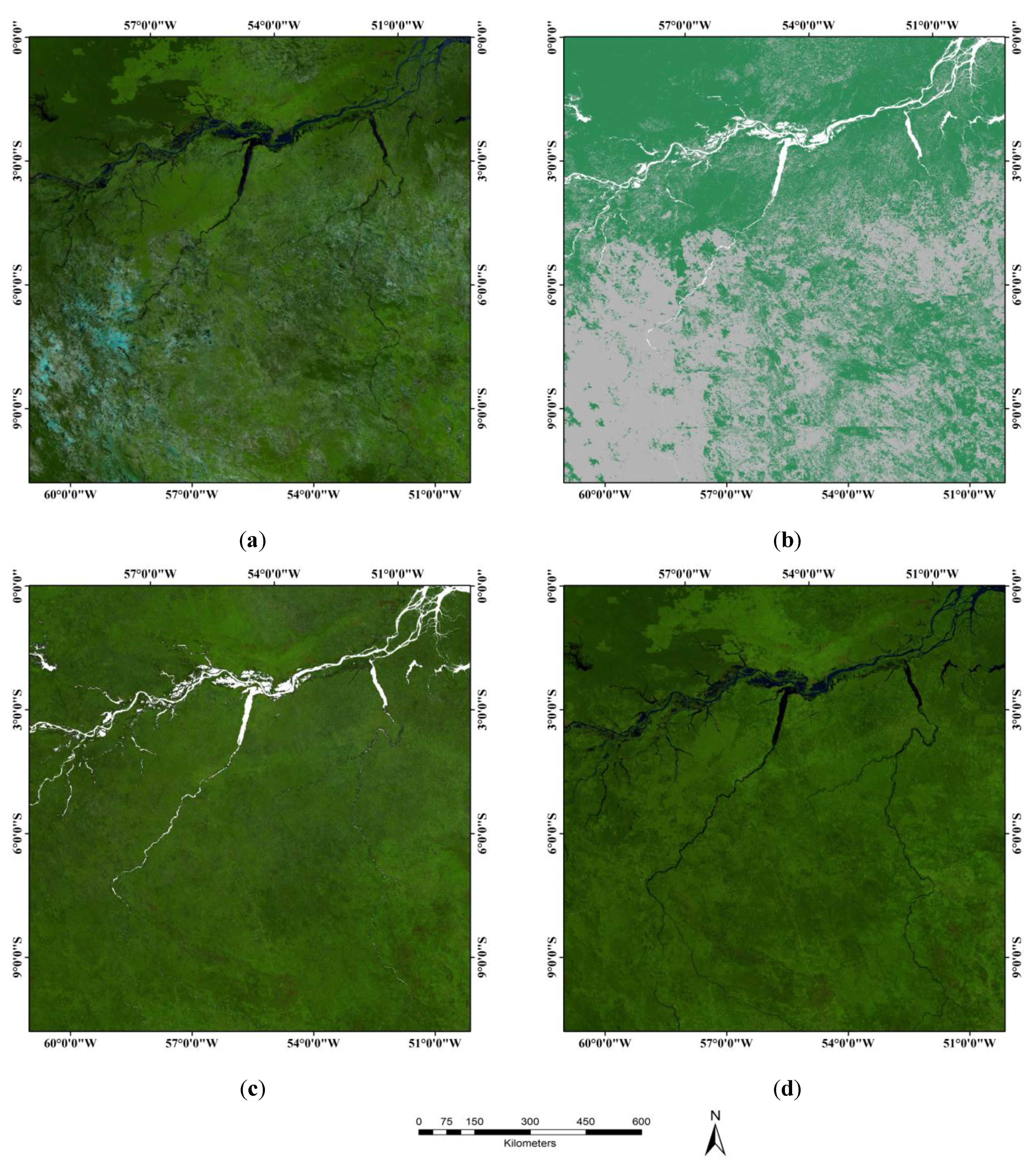
Figure 3 shows the cloud mask and reconstructed surface reflectance for tile h12v09 on day 97, 2003. Figure 3a,c,d is the RGB images of surface reflectance from MOD09A1 and the reconstructed surface reflectance from the VIRR and TSCD methods, respectively. The images were produced with the same RGB color scheme and color enhancement as in Figure 2. In Figure 3a, most of the region was covered by thin clouds, except for several patches in the northwestern area of the image. Figure 3b shows the cloud mask from the VIRR algorithm. The VIRR algorithm effectively identified the thin clouds over this tropical region based on the temporally continuous VIs. The RGB images of the reconstructed surface reflectance data from the VIRR and TSCD methods (Figure 3c,d) show almost all contamination due to clouds was removed.

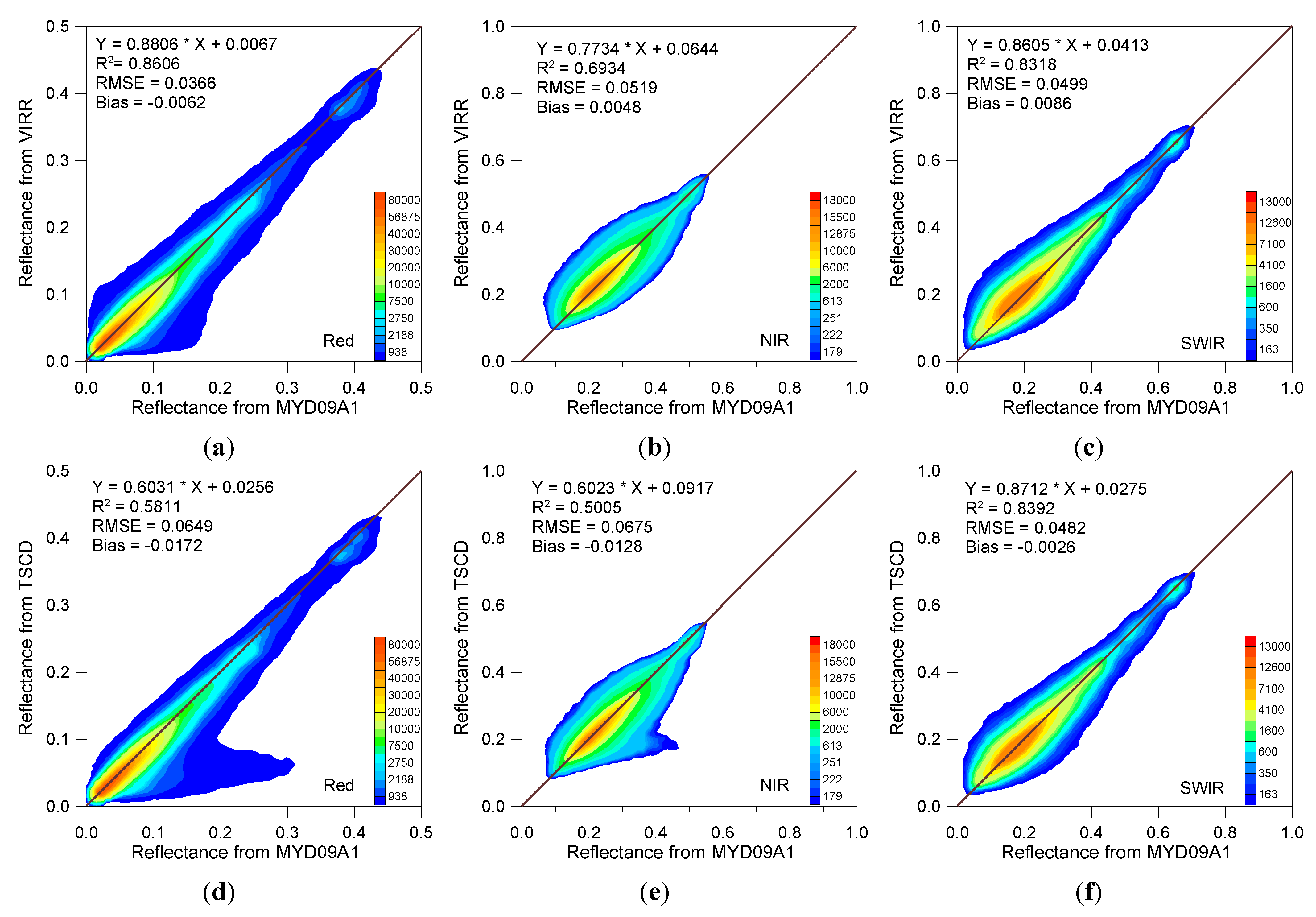
Density scatterplots of the reconstructed surface reflectance from the VIRR and TSCD algorithms versus the cloud-free surface reflectance from MYD09A1 over the BELMANIP sites in 2003 are shown in Figure 4. Only the collocated surface reflectance values from MYD09A1 and the VIRR and TSCD algorithms are included in Figure 4. The density scatterplots between the reconstructed surface reflectance from the TSCD algorithm and the cloud-free surface reflectance from MYD09A1 for the red and NIR bands (Figure 4d,e) show outliers due to underestimation of the reconstructed surface reflectance from the TSCD algorithm. It is apparent that the reconstructed surface reflectance from the VIRR algorithm provides better agreement with the cloud-free surface reflectance from MYD09A1 for the red band (R² = 0.8606 and RMSE = 0.0366) and NIR band (R² = 0.6934 and RMSE = 0.0519) compared with the reconstructed surface reflectance from the TSCD algorithm (R² = 0.5811 and RMSE = 0.0649; and R² = 0.5005 and RMSE = 0.0675, respectively).

Figure 4. Density scatterplots between the cloud-free surface reflectance from MYD09A1 and the reconstructed surface reflectance from the VIRR ((a)–(c)) and TSCD ((d)–(f)) algorithms over the BELMANIP sites in 2003.

Figure 4. Density scatterplots between the cloud-free surface reflectance from MYD09A1 and the reconstructed surface reflectance from the VIRR ((a)–(c)) and TSCD ((d)–(f)) algorithms over the BELMANIP sites in 2003.

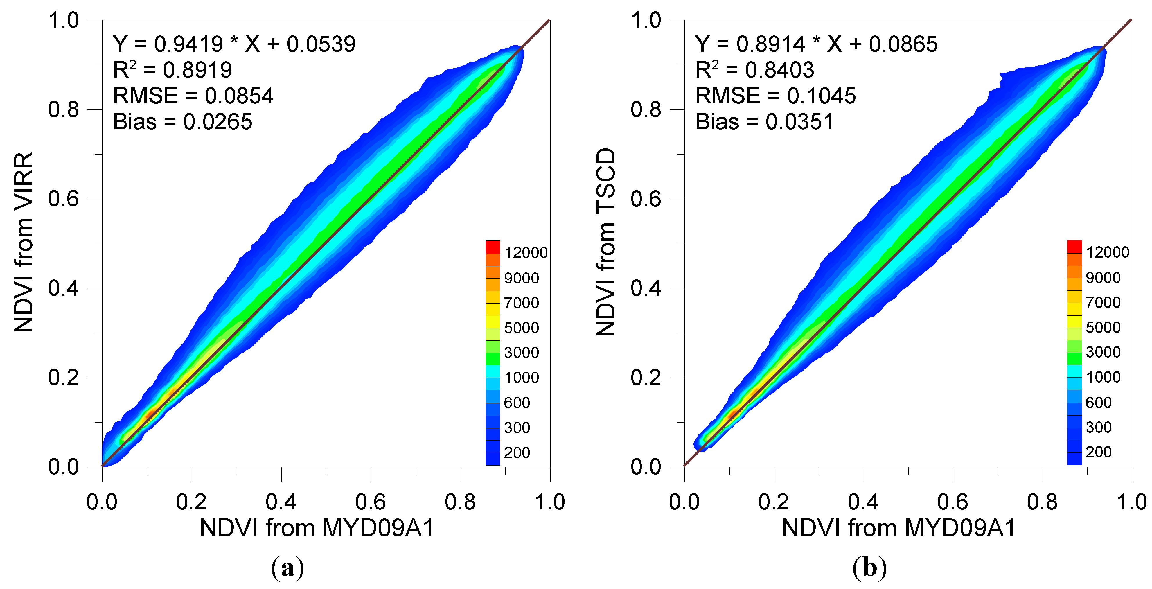
To further assess the consistency of the reconstructed surface reflectance in different bands, NDVI values calculated from the reconstructed surface reflectance were compared with NDVI values calculated from the cloud-free surface reflectance from MYD09A1. Figure 5 shows the density scatterplots of the NDVI values calculated from the reconstructed surface reflectance from the VIRR and TSCD algorithms versus the NDVI values calculated from the cloud-free surface reflectance from MYD09A1 over the BELMANIP sites in 2003. As with Figure 4, the NDVI values from the VIRR and TSCD algorithms are only compared to the collocated NDVI values from MYD09A1. Compared with the NDVI values calculated from the reconstructed surface reflectance from the TSCD algorithm, the NDVI values calculated from the reconstructed surface reflectance from the VIRR algorithm are distributed more closely around the 1:1 line with the NDVI values calculated from the cloud-free surface reflectance from MYD09A1 (with a higher correlation and slope). The NDVI values calculated from the reconstructed surface reflectance from the VIRR algorithm are in better agreement with the NDVI values calculated from the cloud-free surface reflectance from MYD09A1 (RMSE = 0.0854 and Bias = 0.0265) than those calculated from the reconstructed surface reflectance from the TSCD algorithm (RMSE = 0.1045 and Bias = 0.0351).

Figure 5. Density scatterplots of the NDVI values calculated from the reconstructed surface reflectance from the VIRR (a) and TSCD (b) algorithms versus the NDVI values calculated from the cloud-free surface reflectance from MYD09A1 over the BELMANIP sites in 2003.

Figure 5. Density scatterplots of the NDVI values calculated from the reconstructed surface reflectance from the VIRR (a) and TSCD (b) algorithms versus the NDVI values calculated from the cloud-free surface reflectance from MYD09A1 over the BELMANIP sites in 2003.

3.2. Temporal Analysis

In this section, the time series of surface reflectance from MOD09A1 and the reconstructed surface reflectance from the VIRR and TSCD algorithms over a sample of sites with different biome types were presented to further illustrate the performance of the VIRR algorithm. For a better comparison, the time series of NDVI calculated from these surface reflectances are also illustrated over these sites.

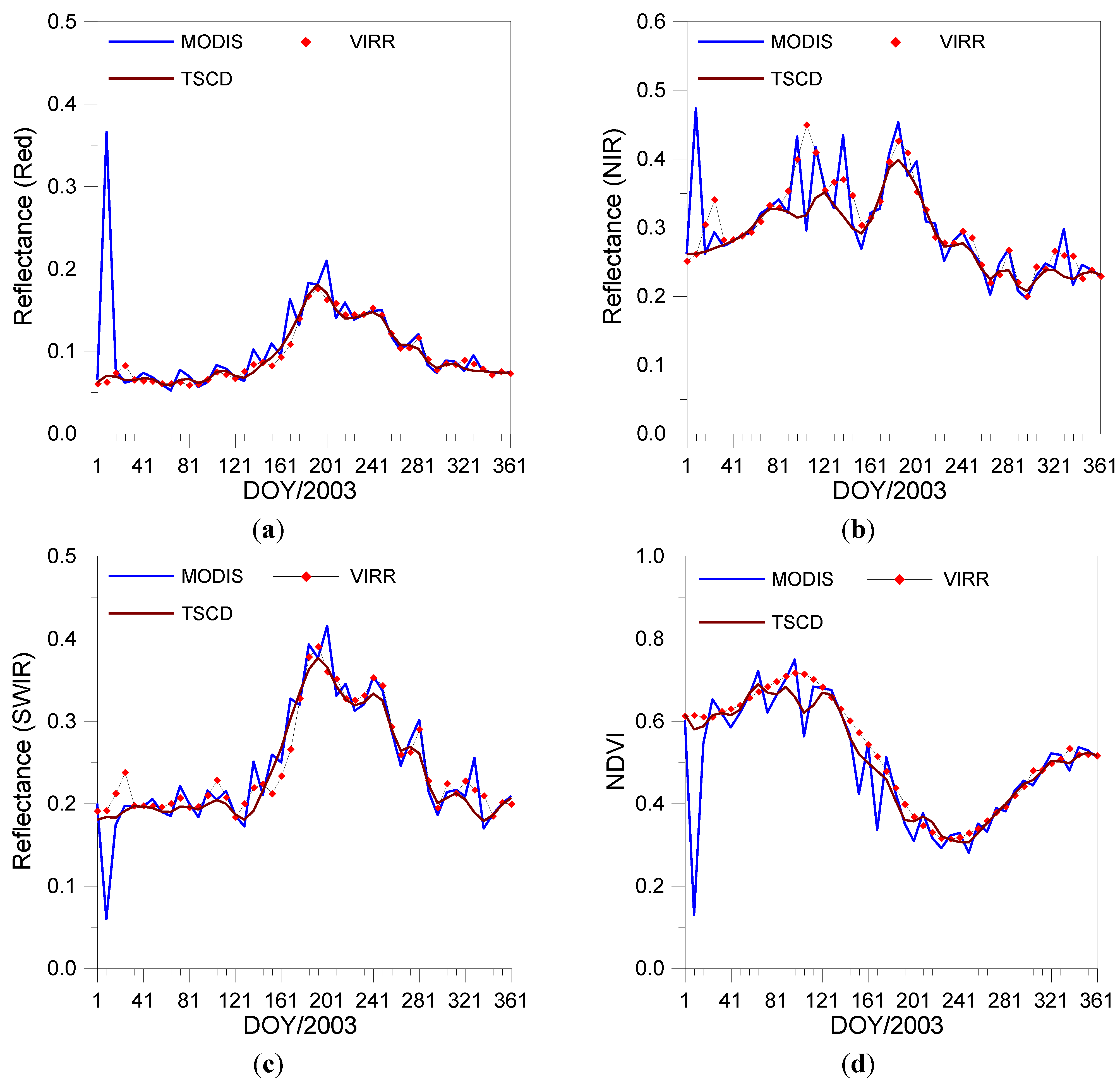
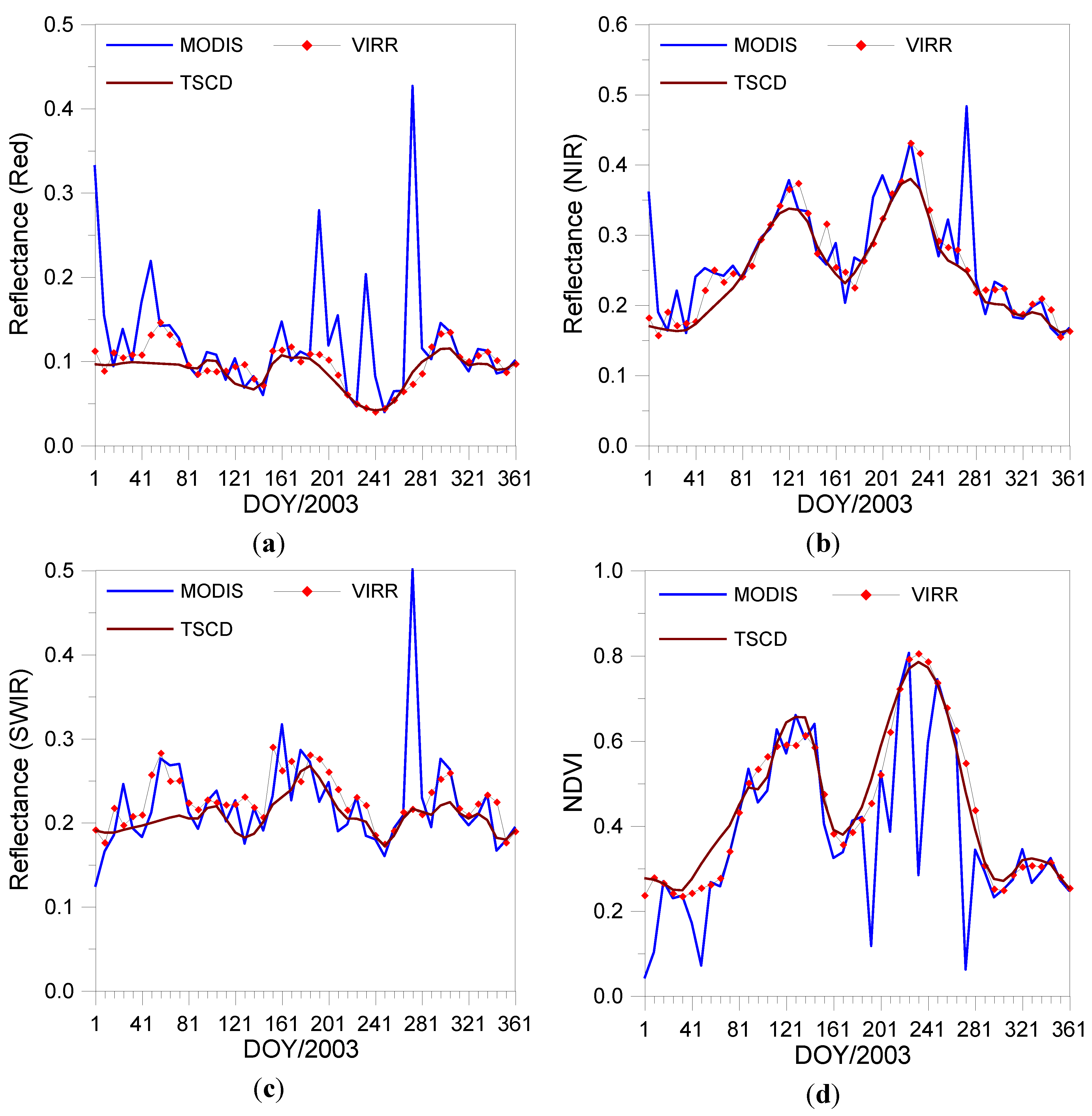
Figure 6 shows the time series of surface reflectance and NDVI for the center pixel of the Alpilles site for the year 2003. The biome type for this site is cropland according to MCD12Q1 product. Figure 6a,c presents the time series of surface reflectance in the red and SWIR bands, respectively. It is observed that the time series of reconstructed surface reflectance from the VIRR method are in good agreement with those from the TSCD algorithm and residual clouds were removed in these reconstructed surface-reflectance data. The time series of surface reflectance in the NIR band are shown in Figure 6b. Some discrepancies between the reconstructed surface reflectance in the NIR band from the VIRR and TSCD algorithm are observed for days 89–153, during which the reconstructed surface reflectance values from the VIRR algorithm were larger than those from the TSCD algorithm. Correspondingly, the NDVI values from the VIRR algorithm were also larger than those from the TSCD algorithm, but the time series of NDVI from the VIRR algorithm was more consistent with the upper envelope of NDVI calculated from MOD09A1 during these days (Figure 6d), which demonstrates that the oscillations in surface reflectance from the VIRR algorithm are physical and related to seasonal variations.

Figure 6. Time series of surface reflectance and NDVI from MOD09A1, the VIRR and TSCD algorithms for the center pixel of the Alpilles site in 2003. (a) surface reflectance in the red band; (b) surface reflectance in the NIR band; (c) surface reflectance in the SWIR band; (d) NDVI.

Figure 6. Time series of surface reflectance and NDVI from MOD09A1, the VIRR and TSCD algorithms for the center pixel of the Alpilles site in 2003. (a) surface reflectance in the red band; (b) surface reflectance in the NIR band; (c) surface reflectance in the SWIR band; (d) NDVI.

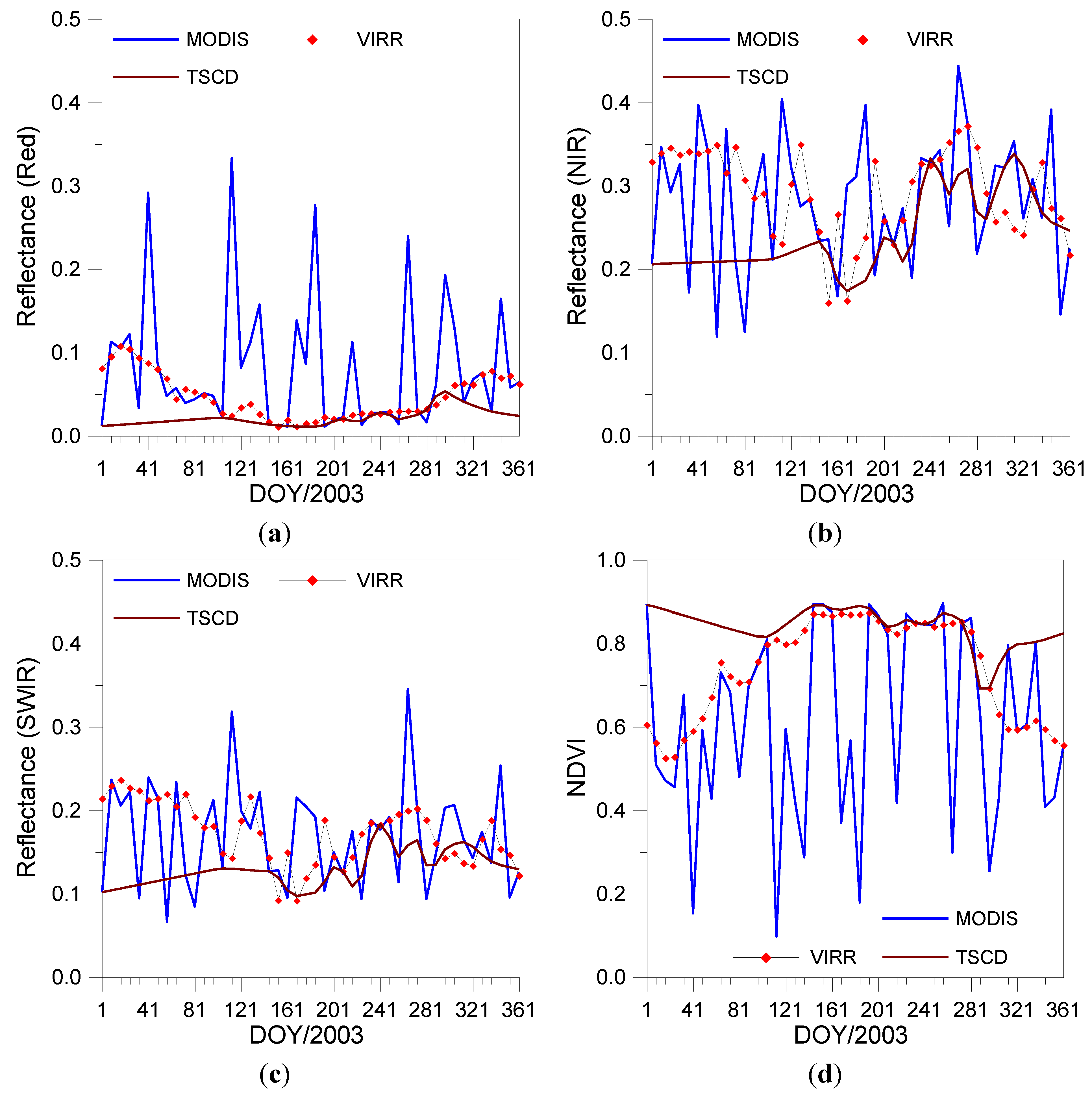
Figure 7. Time series of surface reflectance and NDVI from MOD09A1, the VIRR and TSCD algorithms for the center pixel of the Yucheng site in 2003. (a) surface reflectance in the red band; (b) surface reflectance in the NIR band; (c) surface reflectance in the SWIR band; (d) NDVI.

Figure 7. Time series of surface reflectance and NDVI from MOD09A1, the VIRR and TSCD algorithms for the center pixel of the Yucheng site in 2003. (a) surface reflectance in the red band; (b) surface reflectance in the NIR band; (c) surface reflectance in the SWIR band; (d) NDVI.

Figure 7 shows the time series of surface reflectance and NDVI for the center pixel of the Yucheng site for the year 2003. The biome type for this site is also cropland, but with double annual vegetation seasons, and hence the time series of the surface reflectance and NDVI show seasonal fluctuation. The surface reflectance from MOD09A1, especially in the red band, has several abnormal values at this site (Figure 7a). The VIRR and TSCD algorithms identified those observations with high reflectance values as clouds, and the residual clouds were removed in the reconstructed surface reflectance. However, some discrepancies are also observed. For example, the reconstructed surface reflectance values from the VIRR method are larger than those from the TSCD algorithm for days 33–73 (Figure 7a–c). This is largely due to some clear-sky observations being labeled as clouds by the TSCD algorithm. The corresponding NDVI values calculated from the reconstructed surface reflectance from the TSCD algorithm (Figure 7d) are also larger than those calculated from MOD09A1 and the reconstructed surface reflectance from the VIRR algorithm during those days.

Figure 8. Time series of surface reflectance and NDVI from MOD09A1, the VIRR and TSCD algorithms for the center pixel of the Konza site in 2003. (a) surface reflectance in the red band; (b) surface reflectance in the NIR band; (c) surface reflectance in the SWIR band; (d) NDVI.

Figure 8. Time series of surface reflectance and NDVI from MOD09A1, the VIRR and TSCD algorithms for the center pixel of the Konza site in 2003. (a) surface reflectance in the red band; (b) surface reflectance in the NIR band; (c) surface reflectance in the SWIR band; (d) NDVI.

The time series of surface reflectance and NDVI for the center pixel of the Konza site for the year 2003 are shown in Figure 8. The biome type for this site is grassland according to MCD12Q1 product. On day 33, 2003, the surface reflectance from MOD09A1 in the red band is larger than 0.5, which is most likely cloud. Both the VIRR and TSCD algorithms remove residual clouds in the reconstructed surface reflectance data. However, the TSCD algorithm confirmed that the surface reflectances from MOD09A1 around this day were also contaminated by clouds, as a result of which the reconstructed surface reflectance data from the TSCD algorithm in the red, NIR, and SWIR bands were smaller than those from the VIRR algorithm and MOD09A1 for days 17–105 (Figure 8a–c). Nevertheless, excellent agreement was achieved between the time series of NDVI from both the VIRR and TSCD algorithms for the entire year at this site (Figure 8d).

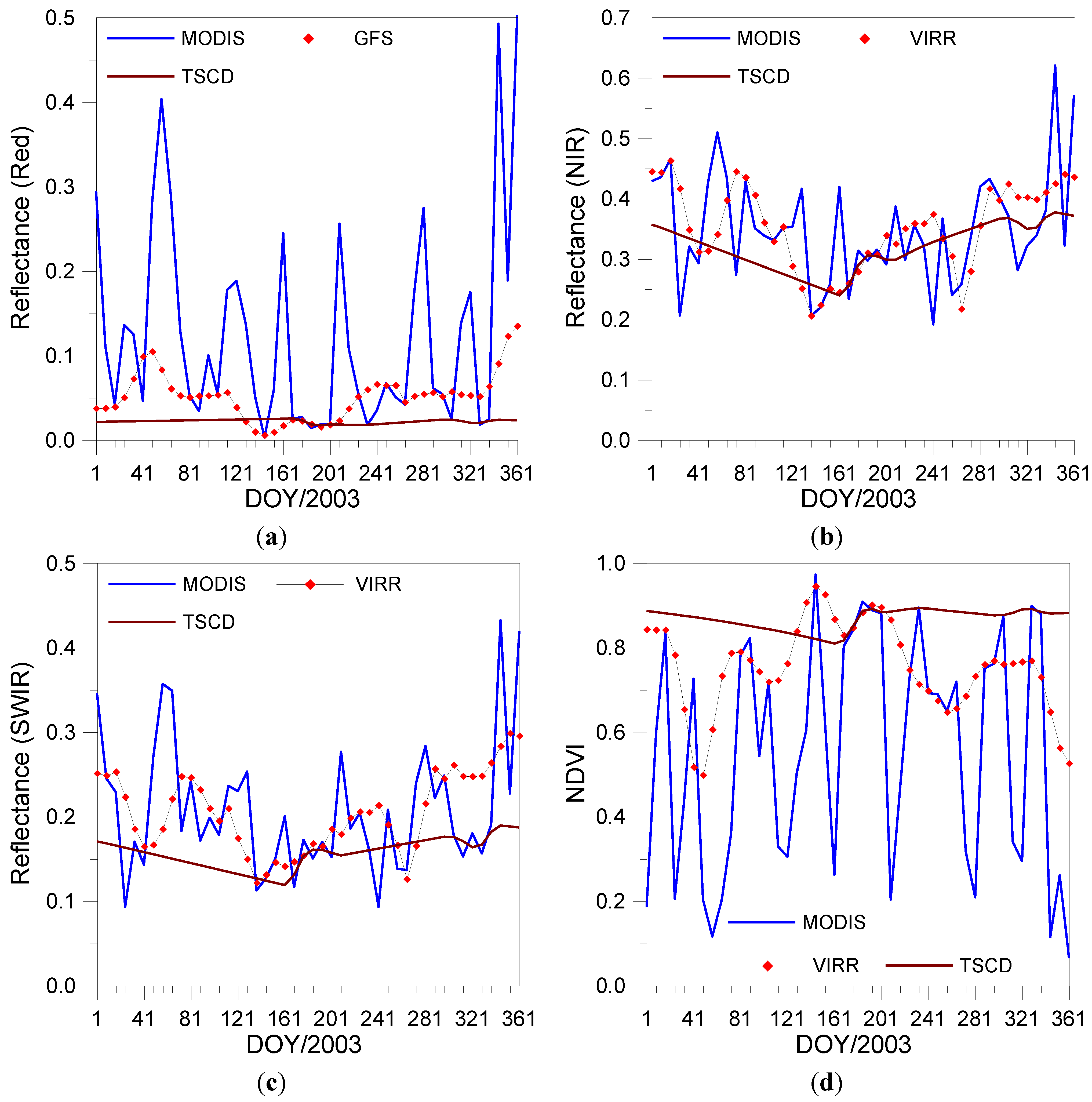
Figure 9. Time series of surface reflectance and NDVI from MOD09A1, the VIRR and TSCD algorithms for the center pixel of the Counami site in 2003. (a) surface reflectance in the red band; (b) surface reflectance in the NIR band; (c) surface reflectance in the SWIR band; (d) NDVI.

Figure 9. Time series of surface reflectance and NDVI from MOD09A1, the VIRR and TSCD algorithms for the center pixel of the Counami site in 2003. (a) surface reflectance in the red band; (b) surface reflectance in the NIR band; (c) surface reflectance in the SWIR band; (d) NDVI.

Figure 9 shows the time series of surface reflectance and NDVI for the center pixel of the Counami site. The biome type for this site is evergreen broadleaf forests according to the MCD12Q1 product. Many residual clouds were observed in the surface reflectance from MOD09A1, and the time series of NDVI from MOD09A1 shows dramatic fluctuations over this site. The reconstructed surface reflectances from the TSCD algorithm are in good agreement with those from the VIRR algorithm after day 145. Large discrepancies are observed before Julian day 145 because of serious contamination due to residual clouds. The TSCD algorithm provides linear surface reflectance values, which cannot address seasonal changes of surface reflectance. However, the VIRR algorithm performed very well to eliminate the effects of clouds, and successfully reconstructed the continuous time series of surface reflectance.

Figure 10. Time series of surface reflectance and NDVI from MOD09A1, the VIRR and TSCD algorithms for the center pixel of the Tapajos site in 2003. (a) surface reflectance in the red band; (b) surface reflectance in the NIR band; (c) surface reflectance in the SWIR band; (d) NDVI.

Figure 10. Time series of surface reflectance and NDVI from MOD09A1, the VIRR and TSCD algorithms for the center pixel of the Tapajos site in 2003. (a) surface reflectance in the red band; (b) surface reflectance in the NIR band; (c) surface reflectance in the SWIR band; (d) NDVI.

Figure 10 shows the time series of surface reflectance and NDVI for the center pixel of the Tapajos site. The biome type for this site is also evergreen broadleaf forests. As with the Counami site, many residual clouds were observed in the MODIS surface reflectance and the time series of NDVI from MOD09A1 showed dramatic fluctuations for the entire year over this site (Figure 10d). It is observed that most of the reconstructed surface reflectance data from the TSCD algorithm change linearly. In contrast, the reconstructed surface reflectance from the VIRR algorithm captures complete and reasonable time series (Figure 10a–c). This, in turn, produces a time series of NDVI in good agreement with the upper envelope of the NDVI from MOD09A1 (Figure 10d).

4. Discussions

The VIRR method is mainly used to reconstruct time series of surface reflectance in vegetated areas for further retrieval of canopy parameters, such as LAI. This study demonstrates that the VIRR method can reconstruct temporally-continuous time series of land-surface reflectance. In fact, the TSCD method is also an effective method to reconstruct the time series of surface reflectance and performs very well, particularly when the land surface is stable or changing slowly [11,12]. However, the TSCD method depends on a rapid change of surface reflectance in the blue band to discriminate between clouded and unclouded pixels. Therefore, the TSCD method cannot be directly used to reconstruct time series of land-surface reflectance data without a blue band. In contrast, a unique feature of the VIRR method is that vegetation indices with obvious seasonal changes are used to identify cloud-contaminated reflectance data and reconstruct time series of surface reflectance. Therefore, whether there are surface reflectance in the blue band and other auxiliary information, or not, the VIRR method is applicable and will be applied to reprocess the MODIS 250 m resolution surface reflectance data and the VIIRS surface reflectance data for LAI retrieval. Another advantage of the VIRR method is that it simultaneously reprocesses multiple-band surface reflectance data, which avoids inconsistent estimation of surface reflectance in the different bands.

Nevertheless, the VIRR method reconstructs the time series of surface reflectance based on the temporally-continuous VIs. Quality of the cloud detection and reconstruction of surface reflectance depends strongly on accuracy of the reconstructed time series VIs especially in areas with data missing over long time periods (such as tropical rain forests).

In addition, the VIRR method aims to correct surface reflectance contaminated by clouds. In fact, the surface reflectance is retrieved from TOA reflectance data through atmospheric corrections which remove the effects of aerosols, thin clouds, and cloud shadows and also introduce additional errors. The uncertainties in the MOD09A1 product have a large impact on the performance of the VIRR method.

5. Conclusions

Current land-surface reflectance products are contaminated with residual clouds, which results in temporal and spatial inconsistencies in subsequent downstream products. This paper developed a new methodology, VIRR, to reconstruct time series of surface reflectance by incorporating the upper envelopes of the time series VIs as constraint conditions. The VIRR method is simple and independent of reflectance data in the blue band and other auxiliary information.

The VIRR method was applied to reprocess the MODIS/TERRA surface reflectance product (MOD09A1). Temporal consistency analysis indicates that the VIRR method successfully removes surface reflectance values contaminated by clouds, and reconstructs temporally-continuous time series of land-surface reflectance. Comparisons with cloud-free surface reflectance from the MODIS/AQUA surface reflectance product (MYD09A1) over the BELMANIP (Benchmark Land Multisite Analysis and Intercomparison of Products) sites in 2003 demonstrate that the VIRR method provides better performance for the red and near-infrared bands than the time series cloud detection (TSCD) algorithm.

In this study, the VIRR method was only applied to reprocess surface reflectance data in the red, near-infrared, and shortwave infrared bands. In the near future, we will extend the methodology to surface reflectance data in other bands. Further considerations of the reconstruction of the MODIS top-of-atmosphere reflectance will be explored in a forthcoming study.