3.3. OM Estimation Based on the Multifield Landscape-Scale Version of MSPA
To achieve high-quality model input data for the MSPA at the landscape scale, the MSPA NDVI-threshold-adapted version of the in-house selection algorithm [
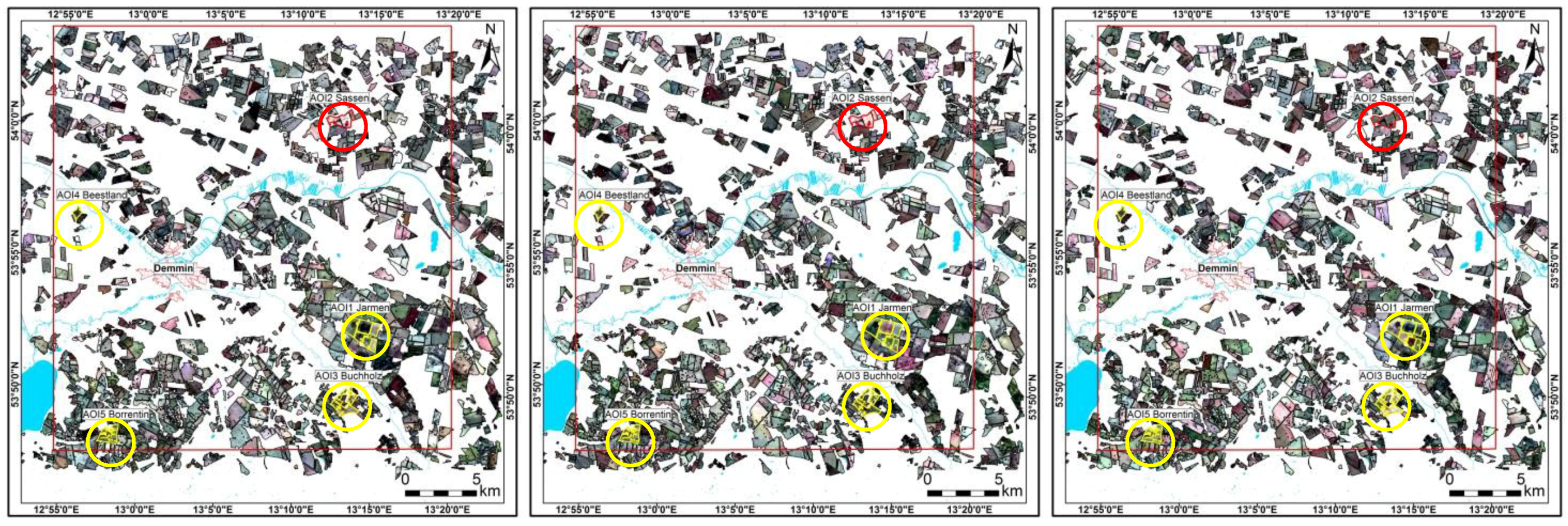
47] was applied to the study area field segments shapefile. Thus, for the NDVI thresholds (MEAN 0.2, SD 0.07), three bare soil image mosaics from lowest to highest SD value were created, applying the modified algorithm to 15 suitable datasets out of the RapidEye time series (
Figure 6).
Figure 6.
Bare soil mosaics for all fields of the study area (red rectangle) including AOI_CAL (yellow polygons/circle) and the validation test site AOI2 (red polygons/circle).
Figure 6.
Bare soil mosaics for all fields of the study area (red rectangle) including AOI_CAL (yellow polygons/circle) and the validation test site AOI2 (red polygons/circle).
These bare soil image mosaics are composed of 1415 field polygons, covering an area of 343.48 km
2. In some polygons, strong temporal patterns (e.g., vital and ripe vegetation and land management) are still visible. The NDVI-MEAN threshold controls the quantity and the quality of the bare soil image per field segment. Reducing this threshold leads to fewer field segments for bare soil image detection (e.g., for NDVI-MEAN 0.15 1151 polygons; for NDVI-MEAN 0.1 569 polygons) and to considerably-diminished strong temporal patterns, such as the presence of vital plants and land management. Despite the substantial improvement, the separation between ripe vegetation and bare soil images still remains difficult. Different spectral resolution and position of wavelength of other multispectral remote sensing sensors (e.g., Landsat-8, Sentinel-2) and hyperspectral Earth observation systems (e.g., EnMAP, HISUI, HyspIRI, PRISMA), as well as the combination of multispectral and radar imagery (e.g., ASAR/ENVISAT [
50]), might be promising for improved separation of bare soil and ripe vegetation as well as for detection of land management effects.
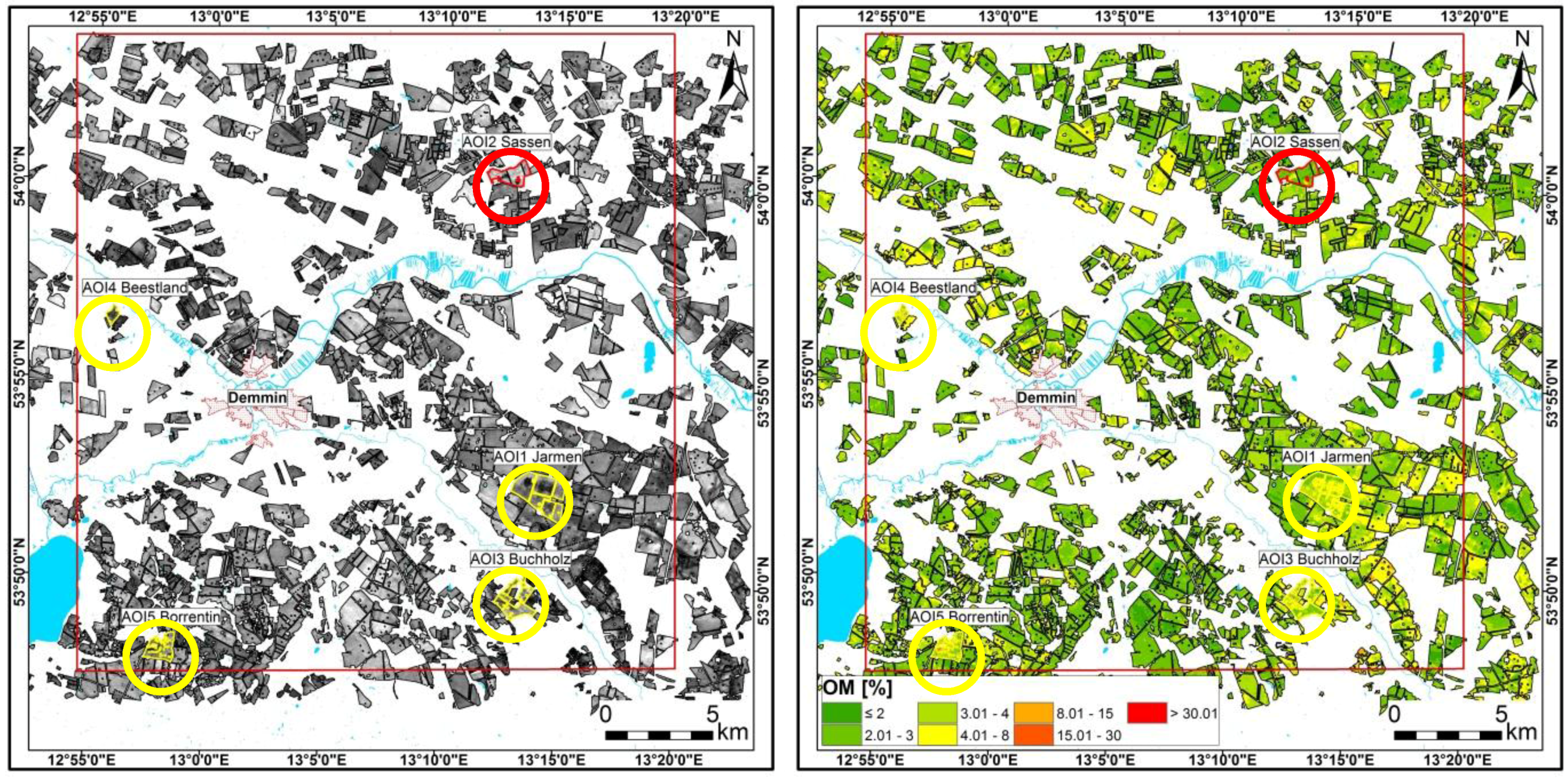
Based on the three PCA-transformed bare soil mosaics (
Figure 7) using the correlation matrix of AOI_CAL (
Table 6), the enhanced regression equation of AOI_CAL was transferred to the study area fields. Thus, a functional soil map of OM was derived and classified with the adaption to the official German Soil Survey Description [
42] (
Figure 7).
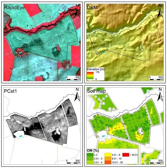
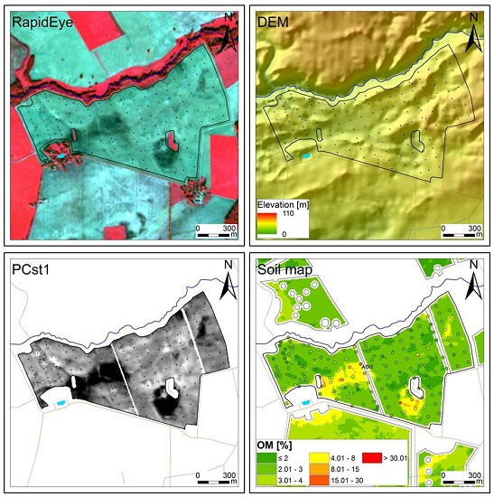
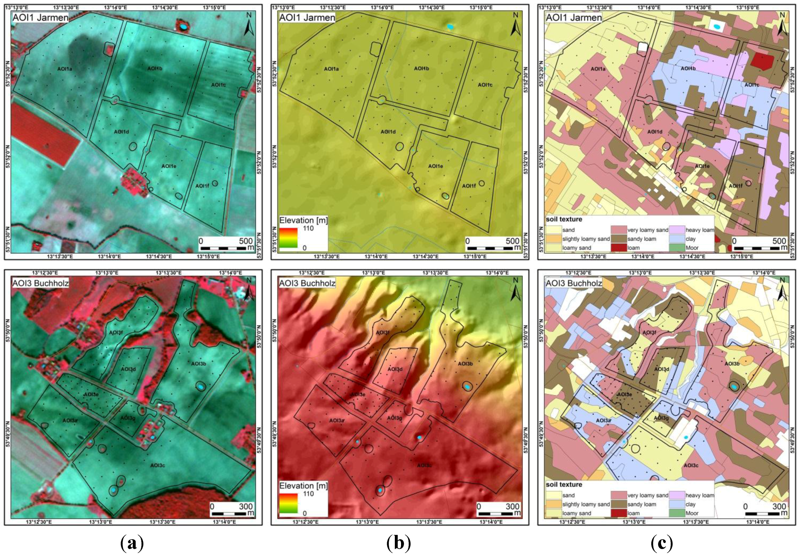
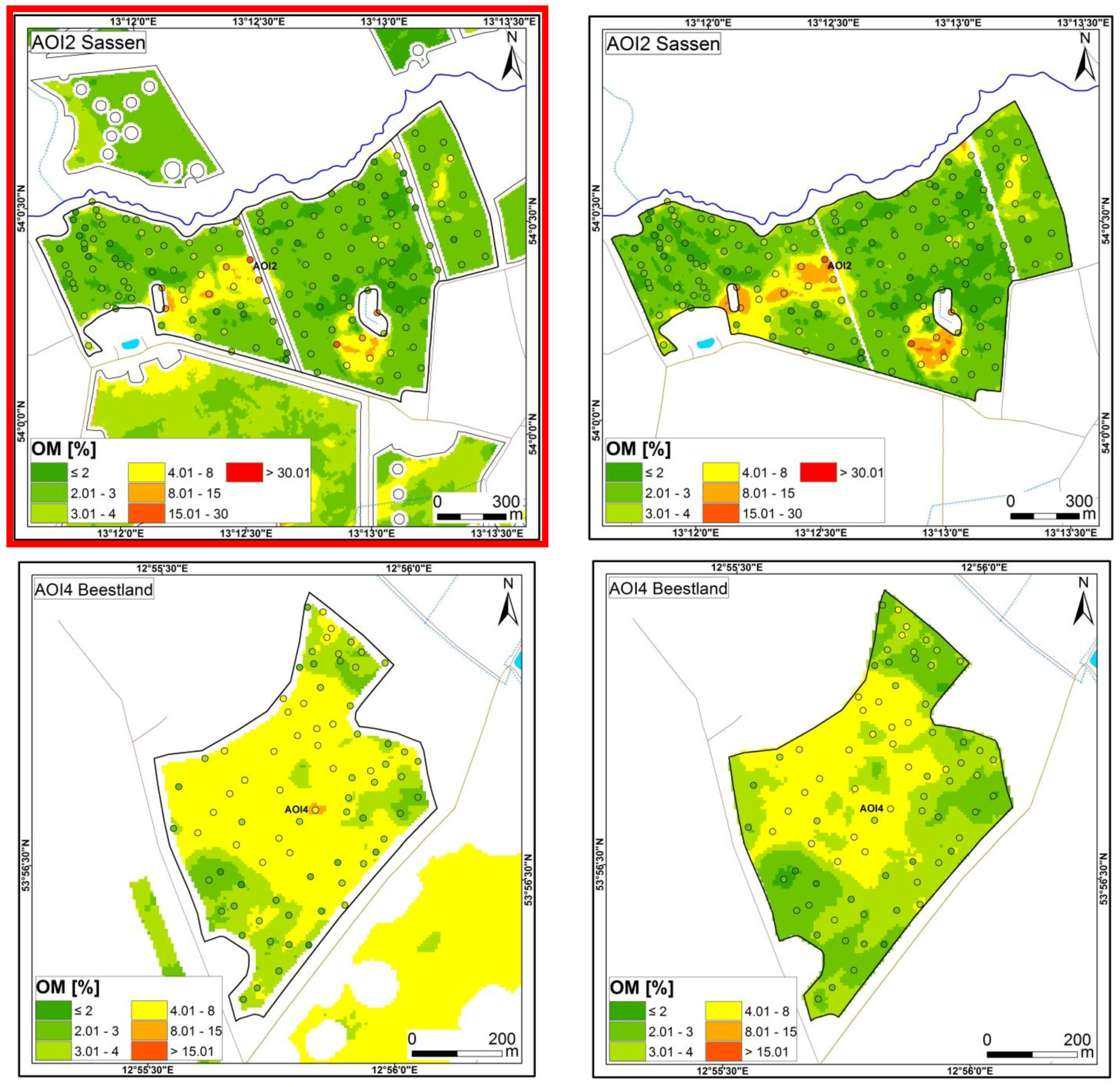
To demonstrate the quality of the OM soil map at the landscape scale based on the regional prediction model and to visualize the behavior of the predicted OM pattern,
Figure 8 shows the map sections of each test site compared with the field-scale OM soil map of each test site based on the test-site-specific prediction model, including the corresponding laboratory-analyzed OM soil sampling results. For the landscape-scale OM soil map the AOI2 test site is the primary validation site, which is not represented in the applied regional prediction model (Chapter 2.5). Consequently, the OM values of this validation test site were modeled in this map independently of the corresponding soil samples.
Figure 7.
(Left) PCst1-transformed bare soil image mosaics of the study area (red rectangle) using the correlation matrix of AOI_CAL (yellow polygons/circle); (right) OM functional soil map based on the regional regression equation (Chapter 3.2) and the PCst1-transformed bare soil image mosaics (OM classification adapted to the official German Soil Survey Description with soil sampling results); validation test site AOI2 (red polygons/circle).
Table 6.
Correlation matrix of AOI_CAL.
Table 6.
Correlation matrix of AOI_CAL.
| 1 | 0.9963 | 0.9960 | 0.9951 | 0.9934 | 0.9876 | 0.9898 | 0.9896 | 0.9910 | 0.9876 | 0.9697 | 0.9746 | 0.9770 | 0.9796 | 0.9727 |
| 0.9963 | 1 | 0.9989 | 0.9986 | 0.9971 | 0.9882 | 0.9916 | 0.9917 | 0.9938 | 0.9904 | 0.9770 | 0.9821 | 0.9839 | 0.9860 | 0.9798 |
| 0.9960 | 0.9989 | 1 | 0.9986 | 0.9970 | 0.9879 | 0.9919 | 0.9928 | 0.9940 | 0.9905 | 0.9768 | 0.9821 | 0.9841 | 0.9860 | 0.9804 |
| 0.9951 | 0.9986 | 0.9986 | 1 | 0.9977 | 0.9870 | 0.9908 | 0.9912 | 0.9946 | 0.9909 | 0.9810 | 0.9856 | 0.9870 | 0.9898 | 0.9842 |
| 0.9934 | 0.9971 | 0.9970 | 0.9977 | 1 | 0.9824 | 0.9866 | 0.9866 | 0.9902 | 0.9886 | 0.9787 | 0.9830 | 0.9840 | 0.9853 | 0.9806 |
| 0.9876 | 0.9882 | 0.9879 | 0.9870 | 0.9824 | 1 | 0.9963 | 0.9955 | 0.9946 | 0.9930 | 0.9612 | 0.9647 | 0.9685 | 0.9714 | 0.9615 |
| 0.9898 | 0.9916 | 0.9919 | 0.9908 | 0.9866 | 0.9963 | 1 | 0.9987 | 0.9980 | 0.9968 | 0.9684 | 0.9720 | 0.9755 | 0.9776 | 0.9686 |
| 0.9896 | 0.9917 | 0.9928 | 0.9912 | 0.9866 | 0.9955 | 0.9987 | 1 | 0.9980 | 0.9962 | 0.9693 | 0.9736 | 0.9772 | 0.9792 | 0.9710 |
| 0.9910 | 0.9938 | 0.9940 | 0.9946 | 0.9902 | 0.9946 | 0.9980 | 0.9980 | 1 | 0.9979 | 0.9766 | 0.9801 | 0.9831 | 0.9857 | 0.9776 |
| 0.9876 | 0.9904 | 0.9905 | 0.9909 | 0.9886 | 0.9930 | 0.9968 | 0.9962 | 0.9979 | 1 | 0.9735 | 0.9755 | 0.9789 | 0.9801 | 0.9717 |
| 0.9697 | 0.9770 | 0.9768 | 0.9810 | 0.9787 | 0.9612 | 0.9684 | 0.9693 | 0.9766 | 0.9735 | 1 | 0.9948 | 0.9939 | 0.9921 | 0.9882 |
| 0.9746 | 0.9821 | 0.9821 | 0.9856 | 0.9830 | 0.9647 | 0.9720 | 0.9736 | 0.9801 | 0.9755 | 0.9948 | 1 | 0.9979 | 0.9971 | 0.9950 |
| 0.9770 | 0.9839 | 0.9841 | 0.9870 | 0.9840 | 0.9685 | 0.9755 | 0.9772 | 0.9831 | 0.9789 | 0.9939 | 0.9979 | 1 | 0.9976 | 0.9942 |
| 0.9796 | 0.9860 | 0.9860 | 0.9898 | 0.9853 | 0.9714 | 0.9776 | 0.9792 | 0.9857 | 0.9801 | 0.9921 | 0.9971 | 0.9976 | 1 | 0.9971 |
| 0.9727 | 0.9798 | 0.9804 | 0.9842 | 0.9806 | 0.9615 | 0.9686 | 0.9710 | 0.9776 | 0.9717 | 0.9882 | 0.9950 | 0.9942 | 0.9971 | 1 |
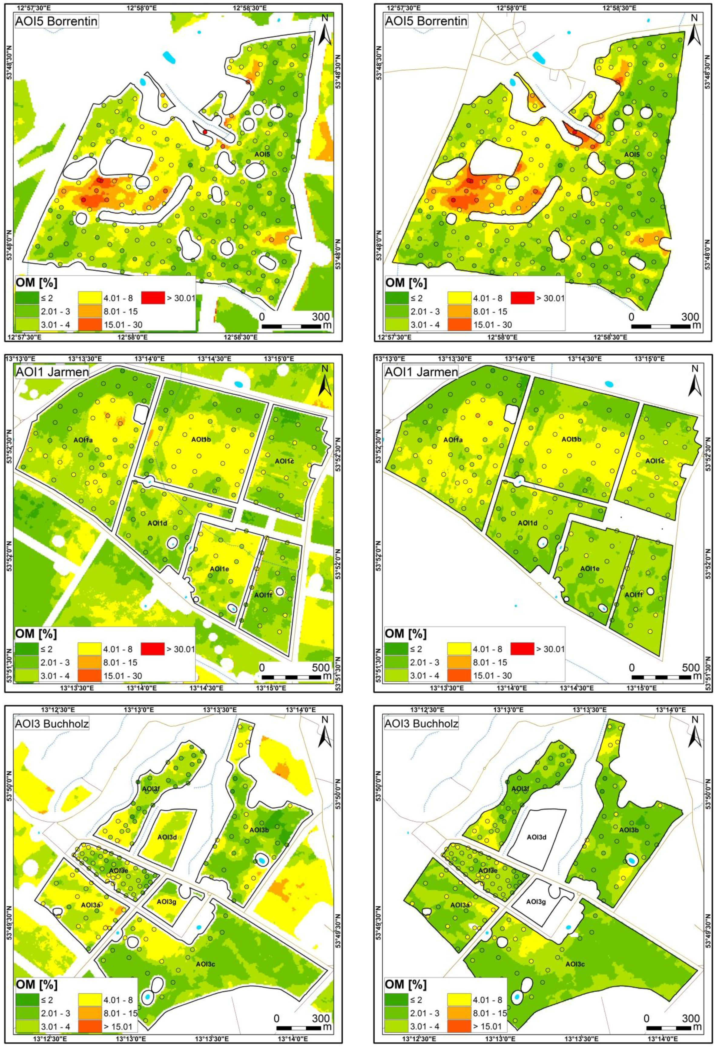
Figure 8.
(Left) Map section of the landscape-scale OM soil map based on the regional prediction model for each test site with the validation test site AOI2 (red rectangle); (right) field-scale OM soil map of each test site based on the test-site-specific prediction model (OM classification adapted to the official German Soil Survey Description with soil sampling results).
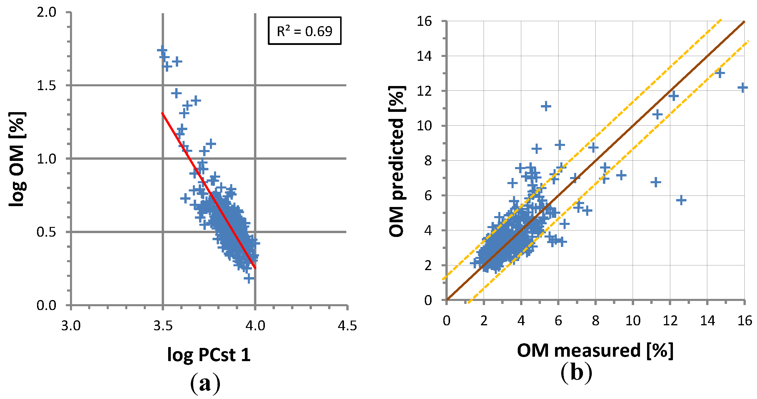
Observing the quality criteria and robustness of the regional (R2 0.69) and local prediction models of AOI1 (R2 0.77), AOI2 (R2 0.72), AOI3 (R2 0.63), AOI4 (R2 0.71), and AOI5 (R2 0.81), besides the significant improvement in the model robustness (especially AOI3, AOI4), a quality decrease from the field scale to the landscape scale based OM maps was expected, with the exception of AOI3.
When checking the mapped and classified OM values, a very similar size and distribution of class zones between the soil maps were noted at the validation test site AOI2, with slight variations at AOI2 (OM classes ≥8.01%), and at the calibration test sites AOI1 and AOI5, with slight changes in the southern field areas (AOI1a, AOI1c) and strong changes in the some field areas of AOI1e and AOI1f. Generally, at AOI3, the majority of the sizes and distributions of the predicted OM class zones had only slight variations; however, in several cases, the same zones were shifted to the next higher OM class (AOI3a, AOI3b, and AOI3f). At AOI4, a strong change in the size and distribution were observed with an increase of the OM class zone from 4.01 to 8.00, particularly in the eastern field.
To assess the classification accuracy of field-scale and landscape-scale based OM maps, confusion matrixes were computed for each test site. For all test sites together,
Table 7 reveals that the overall accuracy (OAA) between both map types differs about 6% (field-scale OAA: 62%; landscape-scale OAA: 56%) with similar slight tendency of overprediction in lower OM classes (≤3.00) and underprediction in higher OM classes (≥4.01). In contrast to the landscape scale classification, the field scale classification contains low underprediction for the OM class 3.01 to 4.00. The higher producer’s accuracy (≥60%) indicates for both maps substantial correct class assignment of corresponding reference samples for the classes 2.01 to 8.00 at the field scale and for the classes 2.01 to 3.00, 4.01 to 8.00, and 8.01 to 15.00 at the landscape scale. Moderate producer’s accuracy (40% to 60%) was obtained for the classes 4.01 to 8.00 (field-scale OM map) and 3.01 to 4.00 (landscape-scale OM map). Except for the classes ≤ 2.00 and 8.01 to 15.00, the probability that a predicted value of the classified OM map actually represents the class of measured value (consumer’s accuracy) is 3% to 15% higher in the field scale OM soil map. As a measure of strength for the relationship between classification results and reference data, the calculated Kappa coefficients of agreement is 0.5 (moderate agreement) for the field scale OM map and 0.4 (moderate agreement) for the landscape scale OM map. The moderate agreement as well as the relatively low OAA result from the prediction error range (absolute RMSE: ≤1.3 OM-%) (
Section 3.1.2) in relation with small class sizes of 1 OM-% for lower OM values. Considering a one-class-classification-error as acceptable, the adjusted OAA increases considerably (field-scale OAA ± 1 class: 98%; landscape-scale OAA ± 1 class: 96%).
The conventional OAAs of the validation test site AOI2 (field-scale OAA: 65%; landscape-scale OAA: 61%) as well as the calibration test sites AOI1 (field-scale OAA: 69%; landscape-scale OAA: 62%) and AOI3 (field-scale OAA: 56%; landscape-scale OAA: 50%) are 4% to 7% more accurate for the field scale maps. AOI4 shows considerable deterioration of 12% (field-scale OAA: 65%; landscape-scale OAA: 43%) due to low image quality of one input bare soil image mosaic with considerable temporal effects of ripe vegetation in the eastern part of the field at the field polygon. The OAA at AOI5 (field-scale OAA: 57%; landscape-scale OAA: 58%) improved about 1% from the field scale to the landscape scale map because of increasing correct value assignment for the class 8.01 to 15.00.
Table 7.
Confusion matrix of the measured OM values (reference) with predicted OM values (classification) for field-scale and landscape-scale based OM soil maps (P.A.: producer’s accuracy, C.A.: consumer’s accuracy).
Table 7.
Confusion matrix of the measured OM values (reference) with predicted OM values (classification) for field-scale and landscape-scale based OM soil maps (P.A.: producer’s accuracy, C.A.: consumer’s accuracy).
| Field-Scale Based OM Soil Map |
|---|
| All Test Sites | Reference (Measured) |
|---|
| ≤2.00 | 2.01–3.00 | 3.01–4.00 | 4.01–8.00 | 8.01–15.00 | 15.01–30.00 | ≥30.01 | Total | C.A. (%) |
|---|
| classification (predicted) | ≤2.00 | 11 | 17 | 1 | 0 | 0 | 0 | 0 | 29 | 38% |
| 2.01–3.00 | 17 | 142 | 39 | 3 | 0 | 0 | 0 | 201 | 71% |
| 3.01–4.00 | 1 | 41 | 108 | 33 | 0 | 0 | 0 | 183 | 59% |
| 4.01–8.00 | 0 | 6 | 33 | 76 | 4 | 1 | 0 | 120 | 63% |
| 8.01–15.00 | 0 | 0 | 0 | 6 | 4 | 3 | 0 | 13 | 31% |
| 15.01–30.00 | 0 | 0 | 0 | 0 | 1 | 2 | 2 | 5 | 40% |
| ≥30.01 | 0 | 0 | 0 | 0 | 0 | 0 | 1 | 1 | 100% |
| total | 29 | 206 | 181 | 118 | 9 | 6 | 3 | 552 | |
| P.A. (%) | 38% | 69% | 60% | 64% | 44% | 33% | 33% | | 62% |
| Landscape-Scale Based OM Soil Map |
| classification (predicted) | ≤2.00 | 8 | 9 | 0 | 0 | 0 | 0 | 0 | 17 | 47% |
| 2.01–3.00 | 19 | 131 | 40 | 2 | 0 | 0 | 0 | 192 | 68% |
| 3.01–4.00 | 2 | 52 | 82 | 26 | 0 | 0 | 0 | 162 | 51% |
| 4.01–8.00 | 0 | 14 | 59 | 82 | 3 | 2 | 0 | 160 | 51% |
| 8.01–15.00 | 0 | 0 | 0 | 8 | 6 | 3 | 0 | 17 | 35% |
| 15.01–30.00 | 0 | 0 | 0 | 0 | 0 | 1 | 3 | 4 | 25% |
| ≥30.01 | 0 | 0 | 0 | 0 | 0 | 0 | 0 | 0 | 0% |
| total | 29 | 206 | 181 | 118 | 9 | 6 | 3 | 552 | |
| P.A. (%) | 28% | 64% | 45% | 69% | 67% | 17% | 0% | | 56% |
3.4. Operability of MSPA for OM Estimation Based on the Regional Prediction Model “Demmin”
According to the crop type and the image acquisition conditions (e.g., signal to noise ratio), the most suitable temporal window of RapidEye data for MSPA at the study area is generally the phase of seeding (winter crops: mid-August to October; summer crops: mid-March to mid-May). Using the found regional prediction model “Demmin” (
Section 3.2), OM can be predicted at the field-scale as well as at the multi-field landscape scale for any single field or field composite of the study area Demmin without additional time-consuming, cost-intensive soil sampling and laboratory analyses.
First, exactly three bare soil images of good quality without any vegetation and/or land management influence are needed. Depending on site-specific characteristics and land management practices, images should not be more than three to five years apart in terms of time, to avoid any OM degradation effects. To create a precise multitemporal bare soil image of the agrarian field of interest without any mixed-pixel influence of field boundary vegetation and/or surrounding trees, all three bare soil images should be stacked together and clipped to the precise extent of the field boundary with a buffer of 20 m. The correlation matrix of AOI_CAL (
Table 6) must be applied as transformation parameters to the standardized PCA of the multitemporal stacked bare soil image, to obtain the field-specific PCst1-image as prediction model input data. Finally, OM soil map can be produced by introducing the PCst1-image to the regression equation of the regional prediction model (
Section 3.2) using for example the Raster Calculator of ArcGIS Spatial Analyst.
Due to the commercial character of the RapidEye satellite system (0.95 €/km
2) [
51], the 54 used RapidEye datasets would cost 42,784.20 € for the study area of 834 km
2. Covering an area of 343.48 km
2, the generated OM soil map at the landscape scale based on the regional prediction model “Demmin” cost 124.56 €/km
2 (namely, 1.25 €/ha) exclusive of additional costs of manpower, working time, soil sampling, and laboratory analyses. In case of the regional model application to any field of the study area, soil sampling, and corresponding laboratory analyses would be redundant. Assuming 20 RapidEye datasets (ordered within the crop type-depending, most suitable temporal window) as sufficient for MSPA application, the costs would range between 4.75 €/ha and 0.95 €/ha for common farm sizes (2000 ha to 10,000 ha) in Mecklenburg-Western Pomerania, taking into account the minimum order size of RapidEye data (500 km
2).
In the future, the combination of the MSPA method with free available Sentinel-2 or Landsat-8 data will enable a high operational use at multiple scales and no cost for image acquisition. This could be improved with the link to locally-developed and/or existing soil spectral libraries such as the European Land Use/Cover Area Statistical Survey database (LUCAS) [
52].


